AI-Driven Optimization for Efficient Public Bus Operations

Abstract

Public transport bus services often experience financial inefficiencies due to high operational costs and unbalanced service allocation. To address these challenges, this study presents a machine learning-based framework aimed at optimizing financial and operational performance in public bus systems. A dataset comprising 57 routes including cost, service, and ridership data was analyzed to identify key factors correlated with net revenue. These features were integrated into multiple predictive models, among which support vector regression (SVR) with a Gaussian kernel and Bayesian optimization achieved the highest accuracy (R² = 0.99), indicating excellent generalization capability. Scenario simulations using the trained SVR model evaluated the effects of service and cost adjustments. Results showed that cutting personnel costs had the most significant effect on net income, followed by administrative and financial expenses. These findings highlight the importance of data-driven strategies such as route reallocation and workforce optimization. The proposed framework offers transit agencies a robust tool for improving efficiency and ensuring financial sustainability.

1. Introduction

With the accelerating pace of global urbanization and the growing emphasis on sustainable development, the operational efficiency and resource allocation of public transport bus services have become critical issues in urban governance [1,2,3,4]. As a primary mode of urban mass transit, bus services significantly influence residents’ travel convenience and quality of life, while also bearing directly on local governments’ fiscal burdens and policy effectiveness [5,6,7]. In densely populated and topographically complex cities, enhancing bus operational performance through scientific management and intelligent decision-making has emerged as a key research focus in the fields of transportation engineering and urban planning [8,9,10].

Traditional studies on bus system performance have primarily relied on conventional statistical analysis and efficiency measurement models such as data envelopment analysis (DEA) and stochastic frontier analysis (SFA) [11,12,13]. These approaches are effective in evaluating relative efficiency but often limited in their ability to handle high-dimensional data and non-linear relationships [14,15]. While traditional analytical approaches have attempted to identify cost centers and suggest improvements, they often fail to provide actionable predictions or account for the non-linear interactions between multiple operational variables [16,17].

With the rapid advancement of data science, machine learning (ML) techniques have gained increasing attention in transportation research for their predictive power and ability to uncover complex patterns [18,19,20]. In this context, machine learning offers a promising alternative to uncover latent patterns within large, complex datasets [21,22,23]. In recent years, deep learning approaches such as Long Short-Term Memory (LSTM), Gated Recurrent Unit (GRU), Convolutional Neural Network (CNN), and Graph Neural Network (GNN) have been widely applied in the transportation domain, particularly for passenger flow prediction and spatiotemporal data modeling, where they demonstrate superior performance compared to traditional methods [18,20]. These methods are highly effective in capturing nonlinear and dynamic relationships and tend to excel when trained on large-scale datasets [17,19,24].

However, few studies have applied ML to analyze Taiwan’s municipal bus systems, and even fewer have considered financial performance as a core outcome variable [25]. Applications include demand forecasting, route optimization, cost control, and service quality assessment. Among these, support vector regression (SVR) is particularly noted for its effectiveness in capturing non-linear relationships with limited training data and strong generalization capability [24,26,27,28,29,30,31]. This study employs a machine learning-based approach to analyze operational data from 57 urban bus routes in Keelung City for the year 2023. An SVR model is constructed to predict net revenue, with parameter tuning and model validation conducted to ensure robustness and accuracy. Additionally, scenario-based simulations are performed to examine the impacts of service frequency. The main contributions of this study are as follows: (1) it presents an integrated machine learning framework for evaluating the financial and operational performance of urban bus systems; (2) it develops a predictive model for net revenue using support vector regression (SVR), leveraging comprehensive operational and cost-related data; and (3) it assesses the financial impacts of various adjustment strategies, such as service frequency modification and cost reduction, and provides concrete policy recommendations. The findings not only offer insights for future policy formulation in Keelung City but also serve as a reference for smart transportation planning and performance improvement in other urban regions.

2. Study Area and Dataset

Keelung City, located in northern Taiwan, faces unique challenges in urban transport planning due to its mountainous terrain, high population density, and frequent rainfall. The public bus system, managed by one of Taiwan’s few remaining public-sector transit authorities, has long operated under fiscal stress, with most routes incurring annual losses. Despite its importance in ensuring social equity and mobility, the city’s bus system suffers from low operational efficiency and limited strategic resource deployment.

The city operates 57 urban bus routes serving a total of 979 bus stops. The system is managed by the Keelung City Public Bus Administration, one of only two remaining publicly operated bus systems in Taiwan, thereby attracting particular attention regarding its operational performance. The primary transit hubs in Keelung are the Keelung Railway Station and the Qidu Railway Station, as illustrated in Figure 1.

According to operational data from 2023, this study collected and analyzed a total of 1083 data records from 57 bus routes in Keelung City. For each route, 15 cost-related variables, along with passenger-kilometers, vehicle-kilometers, ridership, and net income, were compiled. The operational data indicated that the bus system in the city operated under a financial deficit, with each route generating an average net loss of approximately NT$3,419,917.

To improve operational efficiency, this study compiled a dataset consisting of 19 operational and financial variables, including fuel cost, vehicle depreciation, driver-related expenses, maintenance materials, equipment depreciation, maintenance-related expenses, administrative staff salary, driver salary, business staff salary, maintenance staff salary, business expenses, administrative expenses, taxes and duties, depot rental, financial costs, vehicle-kilometers traveled, passenger-kilometers traveled, total ridership, and net revenue, as listed in

Table 1. Datasets used in this study.

		Factor	Description
Vehicle and maintenance costs	Factor 1	Fuel	Bus fuel or energy consumption costs
	Factor 2	Vehicle depreciation	Amortization of bus purchase costs
	Factor 3	Operating-related expenses	Additional operating-related expenses (e.g., insurance premiums)
	Factor 4	Repair materials	Costs of parts and materials for bus maintenance
	Factor 5	Depreciation of equipment	Depreciation costs of office and station equipment
	Factor 6	Ancillary repair expenses	Additional expenses in the repair process (e.g., tool maintenance)
Personnel costs	Factor 7	Management employee salaries	Salaries of supervisors and management personnel
	Factor 8	Operating personnel salaries	Driver salaries and related allowances
	Factor 9	Administrative staff salaries	Salaries of office and administrative staff
	Factor 10	Maintenance personnel salaries	Salaries and allowances of maintenance personnel
Administrative and financial costs	Factor 11	Operating expenses	Operational management-related costs (e.g., office supplies)
	Factor 12	Management expenses	Administrative management expenses (e.g., communication fees)
	Factor 13	Tax expenses	Business tax and other statutory taxes
	Factor 14	Station rent	Bus station rental fees
	Factor 15	Financial expenses	Interest expenses or loan costs
Operational data	Factor 16	Vehicle-kilometers	Total distance traveled by buses on each route
	Factor 17	Passenger-kilometers	Passenger count × travel distance for each bus route
	Factor 18	Passenger count	Passenger count for each bus route
Financial income	Factor 19	Net income	Net income for each bus route

.

Among the 15 cost-related variables, the original data for Factors 7, 9, 10, 11, 12, 13, 14, and 15 were reported as the total cost of the entire road network, without disaggregated data for individual routes. Accordingly, the cost for each route was allocated based on the proportion of its mileage relative to the total mileage of all routes, so as to derive the corresponding cost for each specific route [32,33]. The remaining input factors were determined directly based on the actual conditions of each route.

Table 2. Descriptive statistics of factors.

	Factor	Mean	Standard Deviation	Minimum	Median	Maximum
Factor 1	Fuel	108.6	30.8	0.0	109.5	174.7
Factor 2	Vehicle depreciation	47.1	13.3	0.0	47.6	75.6
Factor 3	Operating-related expenses	10.0	2.7	0.0	10.1	15.8
Factor 4	Repair materials	76.6	21.4	0.0	77.3	122.7
Factor 5	Depreciation of equipment	5.2	1.5	0.0	5.3	8.4
Factor 6	Ancillary repair expenses	0.0	0.0	0.0	0.0	0.0
Factor 7	Management employee salaries	35.7	10.2	0.0	36.1	57.5
Factor 8	Operating personnel salaries	239.4	80.9	0.0	244.0	412.8
Factor 9	Administrative staff salaries	20.7	6.8	0.0	21.1	35.3
Factor 10	Maintenance personnel salaries	7.3	2.6	0.0	7.4	12.9
Factor 11	Operating expenses	56.2	12.8	0.0	56.3	83.6
Factor 12	Management expenses	24.2	5.4	0.0	24.4	35.8
Factor 13	Tax expenses	0.7	0.2	0.0	0.7	1.1
Factor 14	Station rent	3.8	1.0	0.0	3.9	5.8
Factor 15	Financial expenses	39.7	9.9	0.0	40.3	60.6
Factor 16	Vehicle-kilometers	10.9	13.1	0.2	5.4	46.0
Factor 17	Passenger-kilometers	125.8	185.3	0.2	42.3	687.8
Factor 18	Passenger count	30.4	43.4	0.1	5.9	180.1
Factor 19	Net income	−3,419,917.4	4,289,441.1	−9,818,006	−4,309,681	8,317,715

lists descriptive statistics for 19 factors. Within the 19 factors, fuel (Factor 1) and repair materials (Factor 4) exhibit the highest averages among vehicle and maintenance costs, whereas ancillary repair expenses (Factor 6) are negligible. In personnel costs, operating personnel salaries (Factor 8) dominate at an average of 239.4, far exceeding management employee salaries (Factor 7), administrative staff salaries (Factor 9), and maintenance personnel salaries (Factor 10). Administrative and financial costs highlight substantial variation in operating expenses (Factor 11) and financial expenses (Factor 15), while tax expenses (Factor 13) and station rent (Factor 14) remain comparatively minor.

Operational data reveal skewed demand patterns, with vehicle-kilometers (Factor 16) and passenger-kilometers (Factor 17) showing wide dispersion, passenger count (Factor 18) averaging only 30.4 per route, and net income (Factor 19) exhibiting large variability, with most routes operating at a financial deficit.

2.1. Vehicle and Maintenance Costs

Vehicle and maintenance costs encompass a comprehensive range of expenditures associated with the routine operation and upkeep of bus fleets. Fuel costs represent the financial outlays required for energy consumption, which may include diesel, natural gas, or electricity, depending on the propulsion system utilized. Vehicle depreciation accounts for the systematic allocation of the acquisition cost of buses over their estimated service life, reflecting the gradual decline in asset value.

Operating-related expenditures refer to supplementary costs directly linked to vehicle operation, such as insurance premiums and road usage fees. Costs related to repair materials include expenditures on spare parts and consumables necessary for routine maintenance activities. Depreciation of ancillary equipment pertains to fixed assets—such as administrative offices and station facilities—whose value diminishes over time due to usage and obsolescence. Additionally, ancillary repair costs comprise indirect maintenance-related expenditures, including the servicing and replacement of tools and equipment used in repair operations.

Collectively, these cost components illustrate the breadth of financial and material resources required throughout the lifecycle of public transit vehicles, from procurement through to ongoing operation and maintenance.

2.2. Personnel Costs

Personnel costs represent a critical dimension in the present analysis, encompassing all expenditures related to salaries and employee benefits across various functional roles within the public bus system. Salaries for managerial personnel include compensation for administrative and supervisory staff, as well as individuals involved in back-office operations. Driver compensation consists of base pay, shift differentials, and performance-based incentives provided to bus operators. Salaries for office staff encompass remuneration for administrative and customer service employees, while maintenance personnel costs refer to the fixed wages and supplementary allowances allocated to technical staff responsible for vehicle repair and upkeep. As a major component of operating expenditures, personnel costs play a pivotal role in shaping the financial performance of publicly operated bus services, and thus warrant careful consideration in transport system evaluations.

2.3. Administrative and Financial Costs

Administrative and financial costs represent a category of indirect expenditures that, while not directly attributable to core transit operations, significantly influence the overall cost structure of public bus services. Business expenses encompass routine operational outlays related to administrative management, including expenditures on office supplies, printing, transportation, and procurement activities. Management expenses are generally associated with the consumption of internal resources such as utilities (e.g., electricity and water) and communication services required for daily operations. Tax obligations include statutory payments such as business tax and vehicle license tax, mandated by governmental regulations. Facility rental costs refer to payments made for the lease of essential infrastructure, including parking lots and bus terminal spaces. Financial expenses primarily relate to interest payments on loans and associated banking service charges. Although these costs are not directly incurred through route-level service delivery, they constitute a vital component of total operational expenditures and warrant careful consideration in comprehensive cost analyses.

2.4. Operational Data

Operational data factors serve as key performance indicators for evaluating the effectiveness and efficiency of bus route services. Vehicle-kilometers denote the cumulative distance traveled by all scheduled trips on a specific route over a defined time period, serving as a proxy for service supply. Passenger-kilometers, calculated as the product of the number of passengers and the distance each travels, provide insight into the scale and reach of service utilization. Passenger count, or total ridership, reflects the number of users within a given timeframe and offers a direct measure of demand. Net income—defined as the difference between total revenues and all associated costs—serves as the primary indicator of financial performance and is employed as the target variable in the predictive modeling framework developed in this study.

The integration of these performance metrics with cost variables facilitates a holistic assessment of bus route operations and provides an empirical basis for model training and the formulation of evidence-based policy recommendations.

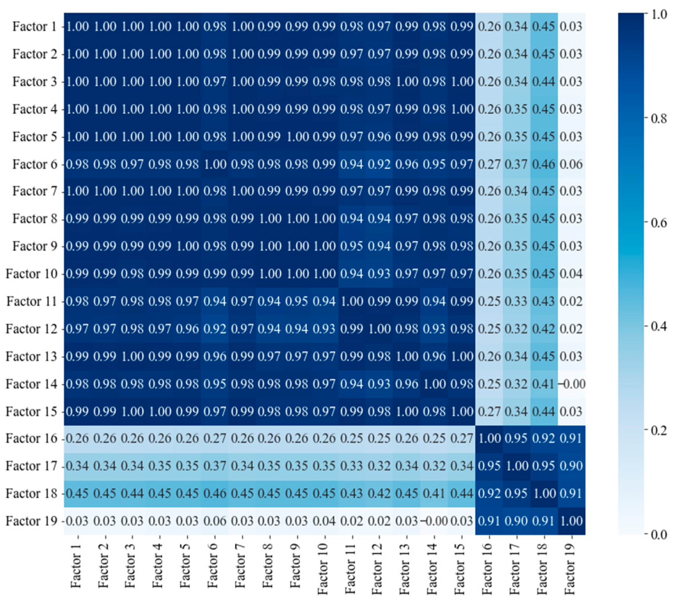
To examine the interrelationships among the factors, Figure 2 presents the correlation matrix. The first 15 factors, which are primarily cost-related, exhibit high degrees of inter-correlation. In contrast, service-related variables, such as vehicle, passenger, and passenger demand, demonstrate only moderate correlations with cost items. Notably, net income, passenger, and passenger numbers are strongly and positively correlated, demonstrating that financial sustainability is driven more by growth in demand than by cost escalation.

3. Development of the ML Model via SVR

Machine learning provides an effective approach to analyzing and predicting bus operation performance, especially in scenarios involving multiple factors and high-dimensional data. This study applies machine learning techniques, using SVR as the primary model, to predict the net income of 57 urban bus routes in Keelung City. The SVR model, known for its excellent generalization ability, tolerance to outliers, and flexibility in handling nonlinear problems, demonstrated high accuracy and stability in this study, making it the optimal choice for net income prediction.

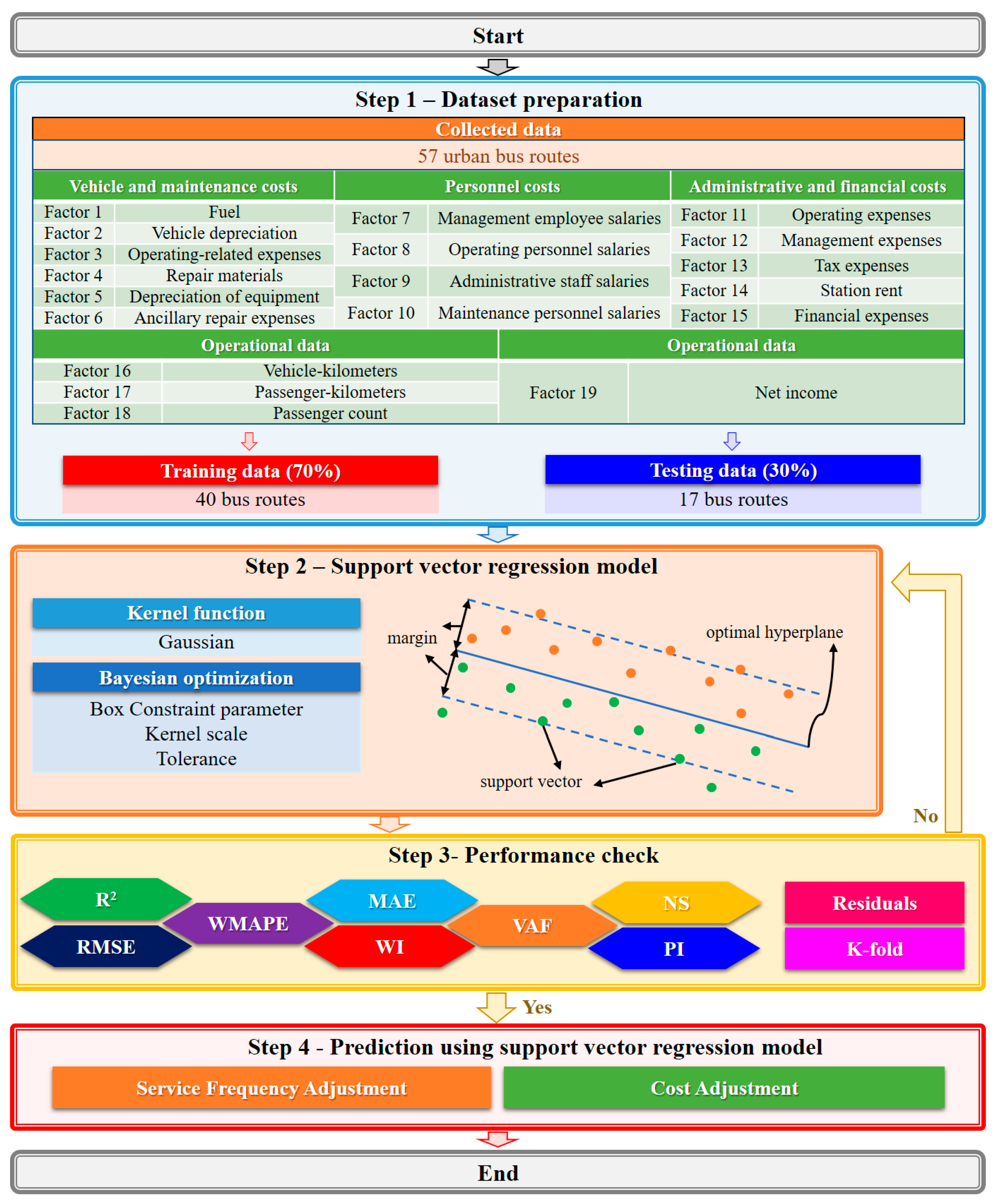
In this study, the SVR model was employed to develop a regression model for bus net income. The SVR is an extension of the support vector machine for regression tasks [32,33,34,35,36]. It employs the loss function to balance model complexity and error tolerance, while kernel functions allow effective modeling of nonlinear relationships. The overall research process includes four main steps: database construction, model training, performance evaluation and model optimization, and application analysis. First, through data collection and organization, a database was constructed, covering 18 input factors, including vehicle and maintenance costs, personnel costs, administrative and financial costs, and operational data, with net income as the output factor. Subsequently, 70% of the data was used for training, and 30% for testing, corresponding to 40 training samples and 17 test samples, with SVR used for model construction. The model’s performance was evaluated using indicators such as R², RMSE, and MAE.

During the model optimization phase, various kernel functions and hyperparameter tuning strategies were compared. The results showed that the Gaussian kernel function combined with Bayesian Optimization yielded the best performance. The model demonstrated high accuracy on the training data and, through K-fold cross-validation (K = 10), confirmed its generalization ability and stability.

Once the model was constructed, application scenario analysis was performed, which included adjustments to bus schedules and cost structures, simulating financial outcomes under different strategies. The results indicated that adjusting the schedules of both high-efficiency and low-efficiency routes, along with reducing specific cost items, could effectively increase overall net income. Figure 3 illustrates the flowchart of this study. The following sections further elaborate on the application process and outcomes of SVR in optimizing bus performance in Keelung City.

4. Validation

4.1. Hyperparameter Optimization of the Model

Hyperparameter optimization is considered crucial for achieving high accuracy during the training process. In the SVR model, optimizing hyperparameters is key to improving model performance and balancing its complexity. This study compares the effects of different kernel functions and selects the kernel function based on the results.

Table 3. Parameters proposed for SVR model.

Parameter	Parameter Value
Kernel function	Gaussian, Linear, and polynomial Kernel function
Optimization method	Bayesian optimization
Box Constraint parameter	218.2
Kernel scale	36.34
Tolerance	5.70 × 10−4

lists the parameters proposed for SVR model. Three types of kernel functions were employed in the modeling process to evaluate their impact on prediction performance: Gaussian, linear, and polynomial kernels. These kernel functions were selected to capture different patterns of nonlinearity and complexity in the data. The hyperparameter optimization was performed using the Bayesian optimization method. The key optimization settings are summarized as follows: the box constraint parameter was set to 218.2, the kernel scale was specified as 36.34, and the convergence tolerance was defined as 5.70 × 10⁻⁴. These parameter choices were aimed at ensuring stable convergence while preserving model generalization capability.

4.2. Model Validation

This study further evaluates the reliability and accuracy of the model using various error metrics, including the coefficient of determination (R²), root mean square error (RMSE), variance accounted for (VAF), prediction interval (PI), mean absolute error (MAE), Willmott index (WI), weighted mean absolute percentage error (WMAPE), and the Nash–Sutcliffe efficiency coefficient (NS). We adopted a broad set of performance measures to capture complementary aspects of model performance. This multi-metric approach reduces bias and strengthens both the credibility and practical relevance of the results. Such indicators are commonly used in machine learning, and the definitions of the eight error metrics are provided in the following section. The goodness of fit of the regression model is assessed using the R², which ranges between 0 and 1. A higher R² value indicates a better fit between the model and the observed data, as follows:

$${\mathrm{R}}^2={\left[{\displaystyle \frac{{\displaystyle \sum _{i=1}^T(d_i-d_{avg})(y_i-y_{avg})}}{\sqrt{{\displaystyle \sum _{i=1}^T{(d_i-d_{avg})}^2}}\sqrt{{\displaystyle \sum _{i=1}^T{(y_i-y_{avg})}^2}}}}\right]}^2$$

(1)

where represents the mean of the actual values of the dependent variable, represents the actual measured values of the dependent variable, represents the mean of the predicted values of the dependent variable, represents the predicted values of the dependent variable, T represents the total number of data points.

RMSE is used to quantify the deviation between observed values and predicted values, calculated by taking the average of the squared differences and then taking the square root, as follows:

$$\mathrm{RMSE}=\sqrt{{\displaystyle \frac{1}{T}}{\displaystyle \sum _{i=1}^T{\left(d_i-y_i\right)}^2}}$$

(2)

VAF is used to quantify the degree to which the independent variables explain the variation in the dependent variable, as follows:

$$\mathrm{VAF}=\left[1-{\displaystyle \frac{\mathrm{SSE}}{\mathrm{SST}}}\right]\times 100$$

(3)

where SSE refers to the sum of squared errors, while SST represents the total sum of squares. A higher VAF value indicates that the independent variables in the model explain a larger proportion of the variation in the dependent variable.

PI represents a range of values used to predict future outcomes at a specific confidence level, as follows:

$$\mathrm{PI}=\left({\displaystyle \frac{\mathrm{VAF}}{100}}\right)+{\hat{\mathrm{R}}}^2-\mathrm{RMSE}$$

(4)

where ${\hat{\mathrm{R}}}^2$ refers to the adjusted ${\mathrm{R}}^2$. MAE is used to evaluate the accuracy of predictions by identifying the maximum absolute error, as follows:

$$\mathrm{MAE}=\max (\left|y_i-d_i\right|)$$

(5)

where max represents the maximum absolute deviation between the predicted values and the observed values.

The WI is a composite metric that combines weighted factors to produce a single score, highlighting the importance of individual contributing elements, as follows:

$$\mathrm{WI}=1-\left[{\displaystyle \frac{{\displaystyle \sum _{i=1}^T{\left(d_i-y_i\right)}^2}}{{\displaystyle \sum _{i=1}^T{\left(\left|d_i-d_{avg}\right|+\left|y_i-d_{avg}\right|\right)}^2}}}\right]$$

(6)

WMAPE is used to quantify the average relative error between the predicted values and the actual values, expressed as a percentage, as follows:

$$\mathrm{WMAPE}={\displaystyle \frac{{\displaystyle \sum _{i=1}^T\left|y_i-d_i\right|}}{{\displaystyle \sum _{i=1}^T\left(y_i\right)}}}$$

(7)

The Nash–Sutcliffe efficiency (NS) is a performance evaluation metric used to assess the degree of agreement between model simulations and observed data. It evaluates the model by calculating the ratio of residual variation to total variation, with a score of 1 indicating ideal model accuracy. A score below 0 indicates that the model’s performance is worse than a simple prediction based on the mean value, as follows:

$$\mathrm{NS}=1-\left[{\displaystyle \frac{{\displaystyle \sum _{i=1}^T{\left(d_i-y_i\right)}^2}}{{\displaystyle \sum _{i=1}^T{\left(d_i-d_{avg}\right)}^2}}}\right]$$

(8)

The predictive model developed in this study demonstrated exceptional performance during both the training and testing phases. Specifically, the model achieved a R² of 0.99 and a RMSE of 7.95 × 10⁻³ in the training phase. Similarly, in the testing phase, it maintained an R² of 0.99 and an RMSE of 4.47 × 10⁻³, indicating high accuracy and robustness. The regression results are illustrated in Figure 4. Furthermore, additional evaluation metrics—including the VAF, PI, MAE, WI, WMAPE, and NS—all reached favorable values, as presented in

Table 4. Optimized Performance evaluation for both training and testing datasets.

Performance Indices	Ideal Value	Training Phase	Testing Phase
R2	1	0.99	0.99
RMSE	0	7.95 × 10−3	4.47 × 10−3
VAF	100	99.90	99.95
PI	2	1.99	1.99
MAE	0	4.05 × 10−3	3.18 × 10−3
WI	1	0.99	0.99
WMAPE	0	1.11 × 10−3	9.91 × 10−3
NS	1	0.99	0.99

, further substantiating the model’s overall predictive efficacy.

The SVR model employed a Gaussian kernel function, with hyperparameters optimized through Bayesian Optimization. The final configuration included a box constraint of 218.2, kernel scale of 36.34, and a tolerance level of 5.70 × 10⁻⁴.

As listed in

Table 5. Performance metrics from K-fold cross-validation.

	Ideal Value	Mean	Standard Deviation
R2	1	0.99	1.08 × 10−3
RMSE	0	5.22 × 10−3	2.31 × 10−4
VAF	100	99.95	1.85 × 10−2
PI	2	1.99	5.89 × 10−3
MAE	0	3.58 × 10−3	1.04 × 10−4
WI	1	0.99	1.01 × 10−3
WMAPE	0	1.25 × 10−3	9.77 × 10−4
NS	1	0.99	7.52 × 10−3

, the high R² values may raise concerns about potential overfitting. However, route-level net income in our dataset is largely driven by service- and demand-related variables. Passenger-kilometers, vehicle-kilometers, and ridership all exhibit strong correlations with net income (correlation coefficients exceeding 0.9, as shown in Figure 2). Given the stable and structured relationships among costs, service provision, and revenue within this system, the model’s high predictive performance is well explained.

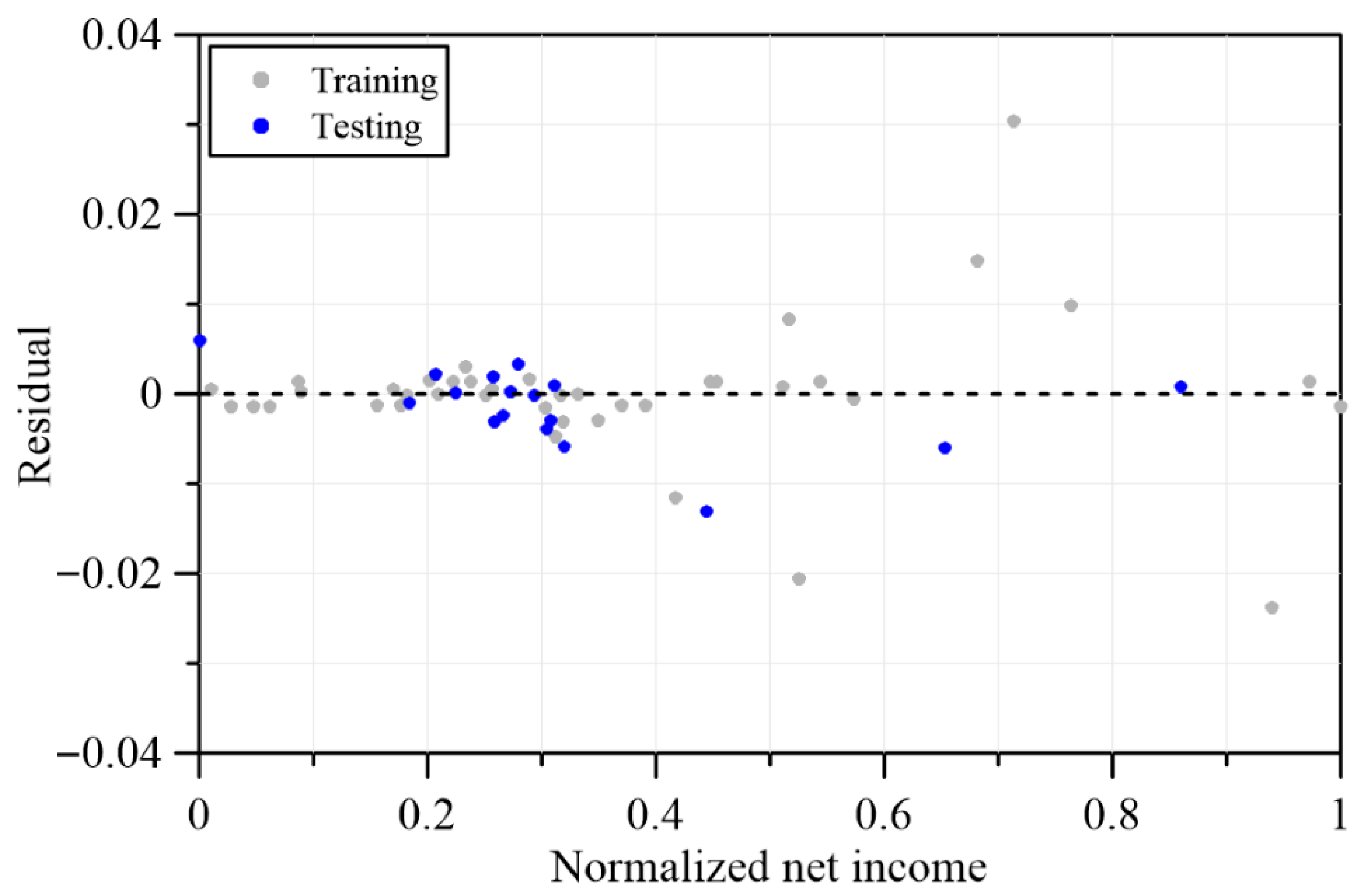
Moreover, this study conducted additional validation. The distributions of the training and testing datasets were examined through visualization (Figure 5) and were found to be highly consistent, with the majority of values concentrated within the range of 0.4 to 0.8. This similarity suggests that the model does not exhibit early convergence or entrapment. In addition, residual error distributions were analyzed for both datasets (Figure 6). The training residuals predominantly ranged between −0.02 and 0.02, whereas the testing residuals ranged between −0.04 and 0.04. The absence of systematic deviations or clusters of extreme errors further indicates that the model is not subject to overfitting.

To further assess robustness, we conducted a 10-fold cross-validation stratified at the route level to prevent data leakage. The results yielded a mean R² of 0.99 with a very small standard deviation (1.08 × 10⁻³), demonstrating stable performance across folds (

Table 6. Comparison of SVR model performance across alternative training-to-testing split ratios.

Training/Testing Split	90/10	80/20	70/30	60/40
R2	0.97	0.99	0.99	0.99
RMSE	5.85 × 10−3	4.92 × 10−3	4.47 × 10−3	4.59 × 10−3
VAF	98.63	99.86	99.95	99.93
PI	1.98	1.99	1.99	1.99
MAE	5.41 × 10−3	4.12 × 10−3	3.18 × 10−3	3.92 × 10−3
WI	0.98	0.99	0.99	0.99
WMAPE	1.06 × 10−2	9.96 × 10−3	9.91 × 10−3	9.95 × 10−3
NS	0.98	0.99	0.99	0.99

). In addition, beyond the original 70/30 split, we performed multiple hold-out validations with alternative ratios (e.g., 60/40, 80/20), which consistently produced comparable results. Since the dataset is cross-sectional at the route level rather than longitudinal, time-based splits are not applicable; instead, robustness was evaluated through repeated hold-outs and K-fold cross-validation as described above.

4.3. Comparison of ML Models

To develop a precise prediction model for the net income of individual urban bus routes in Keelung City, this study compared the predictive performance of four widely used machine learning regression models: SVR, random forest (RF), and artificial neural network (ANN), eXtreme Gradient Boosting (XGBoost), and light gradient boosting machine (LightGBM). Each model was evaluated through 50 repeated tests, and performance was assessed using a range of regression evaluation metrics, including the R², RMSE, VAF, PI, MAE, WI, WMAPE, and NS.

The comparison results indicate that the SVR model outperformed all other models across all evaluation metrics. It achieved an R² of 0.99, an RMSE as low as 5.21 × 10⁻³, and a VAF of 99.92%. Other indicators such as PI, MAE, and WI were also close to ideal values, demonstrating both high predictive accuracy and stability. In contrast, the ANN, and RF models showed relatively inferior performance, as reflected in their higher error rates and lower stability under the same evaluation framework, as summarized in

Table 7. Comparison of results using different machine learning models.

Performance Indices	Ideal Value	SVR	RF	ANN	XGBoost	LightGBM
R2	1	0.99	0.93	0.99	0.98	0.98
RMSE	0	5.21 × 10−3	6.34 × 10−2	1.17 × 10−2	2.54 × 10−2	2.69 × 10−2
VAF	100	99.92	93.11	99.70	98.70	99.87
PI	2	1.99	1.96	1.99	1.99	1.99
MAE	0	3.52 × 10−3	4.51 × 10−2	6.97 × 10−3	7.52 × 10−3	6.51 × 10−3
WI	1	0.99	0.98	0.99	0.98	0.98
WMAPE	0	1.24 × 10−2	1.22 × 10−1	2.74 × 10−2	3.15 × 10−2	4.52 × 10−2
NS	1	0.99	0.93	0.99	0.99	0.99

.

The main reasons for the poorer performance of ANN, RF, and XGBoost may lie in the interaction between dataset characteristics and model assumptions. Specifically, our dataset is relatively small, where SVR is well known for its strong generalization capability under small-sample, high-dimensional conditions. In contrast, ANN and XGBoost typically require larger datasets to avoid overfitting and to fully utilize their capacity, which limited their effectiveness in this study. Furthermore, the Gaussian kernel in SVR effectively captures nonlinear relationships between financial and operational variables, while RF and XGBoost may also model nonlinearities but tend to produce less stable results when sample size is limited and variable interactions are complex.

In conclusion, the SVR model proved most suitable for predicting bus route net income in Keelung City. Its superior performance across evaluation metrics reflects a better fit to the scale and characteristics of our dataset, offering high accuracy and robust generalization that provide a reliable basis for scenario analysis and policy recommendations.

5. Application Example

To validate the effectiveness of the SVR model developed in this study for predicting net income in bus operations, this section introduces two major scenario-based simulation strategies: service frequency adjustment and cost adjustment. By modifying operational parameters, the analysis aims to evaluate the extent of improvement in overall financial performance and to provide concrete policy recommendations.

5.1. Scenario Simulation: Service Frequency Adjustment

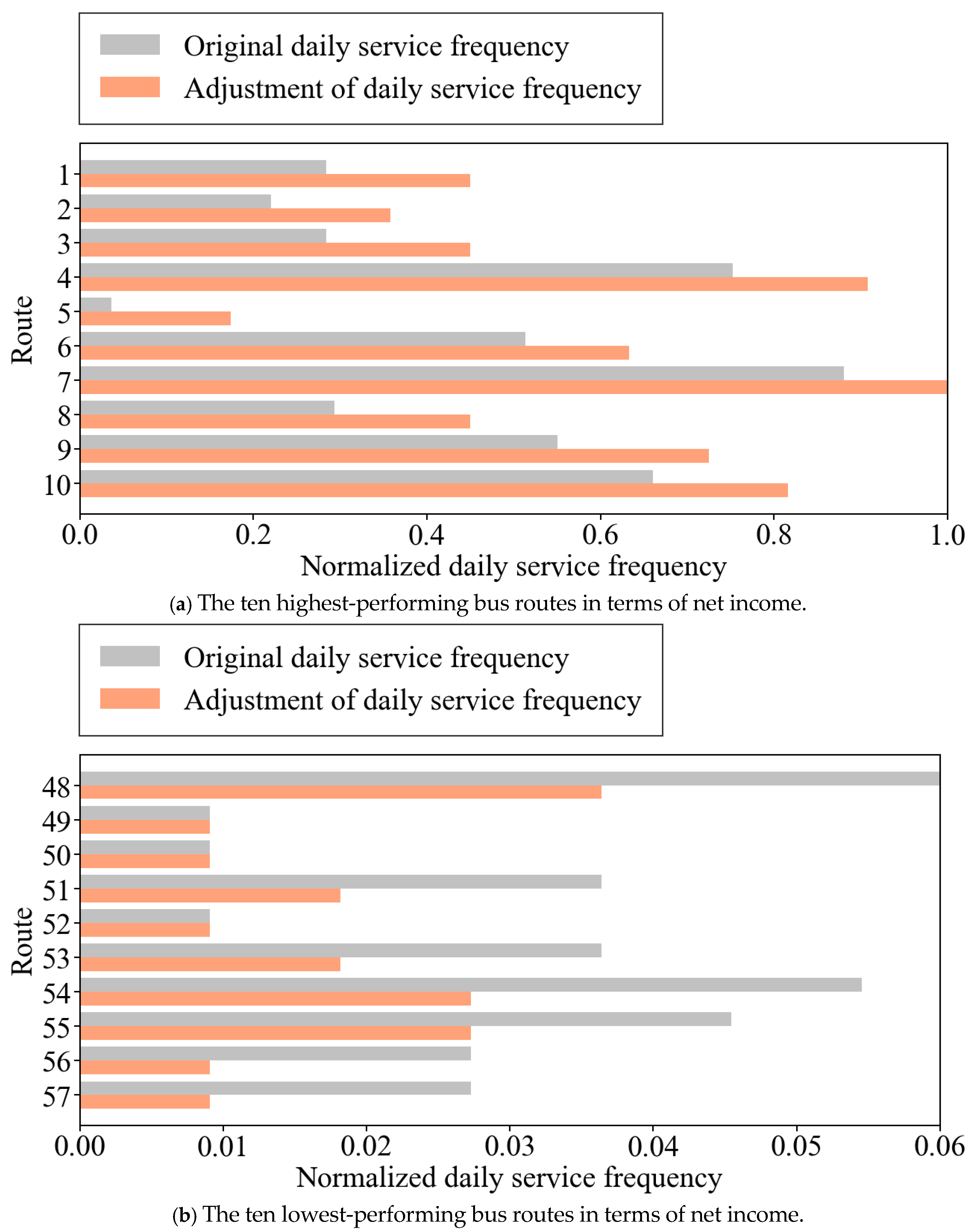
According to the Keelung City Public Bus Administration, the city operates a total of 57 urban bus routes. This study selected the top 10 most profitable and the bottom 10 least profitable bus routes, based on net income rankings, to conduct a scenario simulation.

As illustrated in Figure 7, the simulation focused on adjusting service frequency to evaluate the impact of resource reallocation on overall net income. The y-axis indicates the corresponding bus routes. The x-axis represents the normalized daily service frequency, defined as the number of daily trips for each bus route divided by the maximum number of daily trips among all routes, as formulated in Equation (9):

$$\mathrm{Normalized} \mathrm{daily} \mathrm{service} \mathrm{frequency}={\displaystyle \frac{S{F}_i}{S{F}_{\max }}}$$

(9)

where $S{F}_i$ denotes the number of daily service frequency for bus route i, and $S{F}_{\max }$ represents the maximum number of daily service frequency among all bus routes. In this study, Equation (9) normalizes service frequency relative to the maximum observed value to ensure a consistent comparison across routes and to avoid bias toward high-frequency services. As shown in Table 2, we examined that the maximum frequency was not an outlier, thereby minimizing the risk of distortion. Moreover, the analysis emphasizes relative changes in service frequency before and after adjustment rather than absolute values, ensuring that the normalization does not compromise the validity of the policy implications. The adjustment strategy involved increasing the service frequency for high-performing routes, specifically Routes 1 through 10, as shown in Figure 7a, while moderately reducing or maintaining the frequency for low-performing routes, namely Routes 48 through 57, as illustrated in Figure 7b.

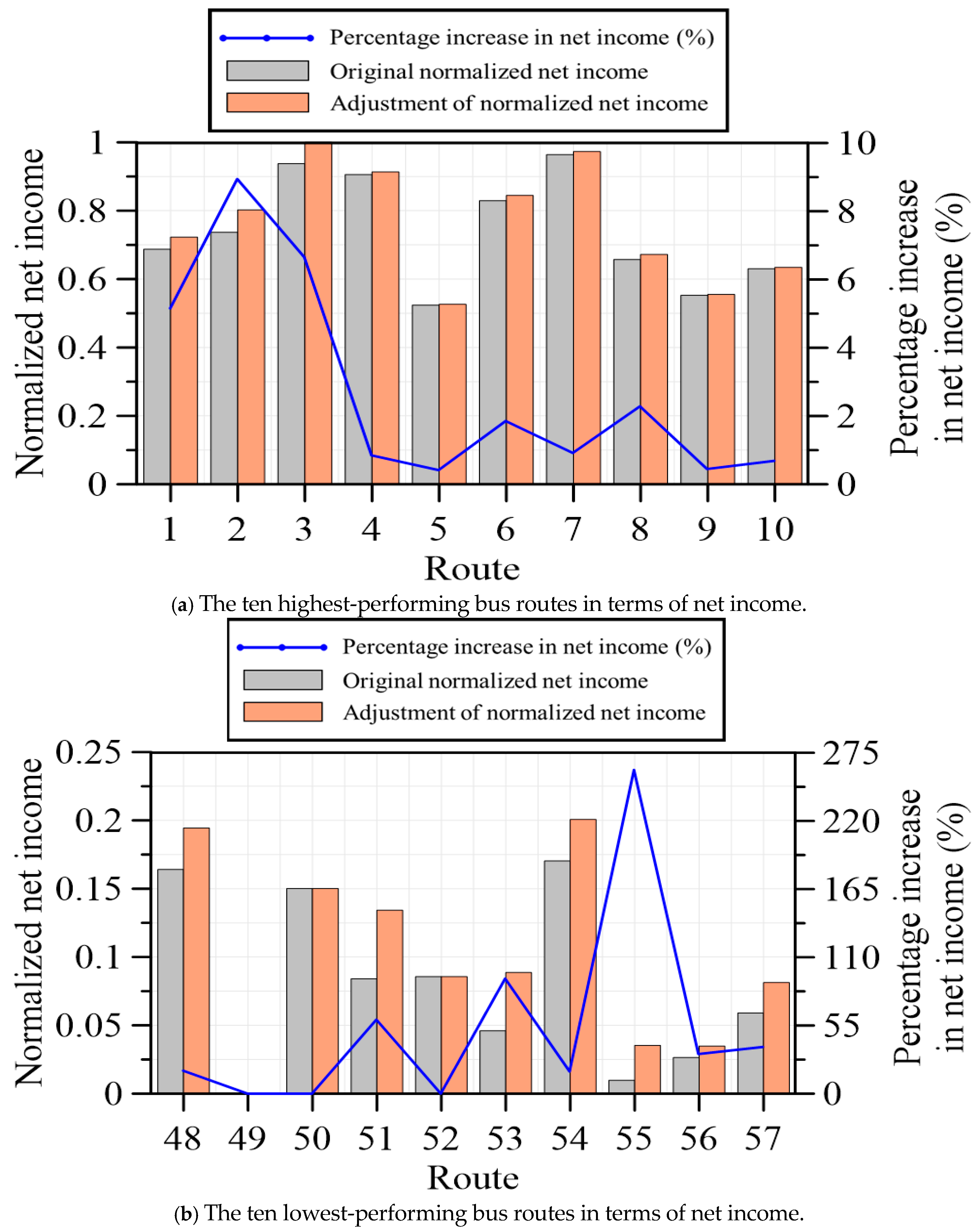
Figure 8 shows the comparison of net income before and after service frequency adjustment. The x-axis indicates the corresponding bus routes, while the y-axis on the left represents the normalized net income, as formulated in Equation (10):

$$\mathrm{Normalized} \mathrm{net} \mathrm{income}={\displaystyle \frac{N{I}_i-N{I}_{\min }}{N{I}_{\max }-N{I}_{\min }}}$$

(10)

where $N{I}_i$ denotes the net income of bus route i, $N{I}_{\min }$ is the minimum net income among all bus routes, and $N{I}_{\max }$ is the maximum net income among all bus routes. The y-axis on the right side of Figure 8 represents the percentage increase in net income, which can be expressed by Equation (11) as follows:

$$\mathrm{Percentage} \mathrm{increase} \mathrm{in} \mathrm{net} \mathrm{income} (\%)={\displaystyle \frac{N{I}_{before}-N{I}_{after}}{N{I}_{before}}} \times 100 \%$$

(11)

where $N{I}_{before}$ denotes the net income before adjustment, and $N{I}_{after}$ denotes the net income after adjustment. The post-adjustment results, as illustrated in Figure 8, demonstrate a significant improvement in net income following the implementation of service frequency adjustments. Figure 8a presents a comparative analysis of net income before and after adjustment for the ten highest-performing bus routes, revealing moderate yet consistent gains in profitability. Figure 8b illustrates the corresponding comparison for the ten lowest-performing bus routes.

Notably, the results indicate that routes with initially low net income experienced substantial improvements when service frequencies were moderately reduced. In several cases, the percentage increase in net income was particularly pronounced, suggesting that scaling back operations on underperforming routes can effectively reduce operating costs while maintaining essential service coverage. This finding highlights the potential of demand-responsive strategies in public transport planning. Overall, the observed improvements across both high- and low-performing routes underscore the effectiveness of strategic resource reallocation in optimizing network-wide performance. The increase in the total net income of Keelung City’s urban bus system confirms that data-driven frequency adjustments can significantly enhance operational efficiency and financial sustainability. These results provide empirical support for implementing adaptive transit management strategies aimed at improving the cost-effectiveness of urban bus systems under constrained resources.

5.2. Cost Adjustment Scenario Simulation

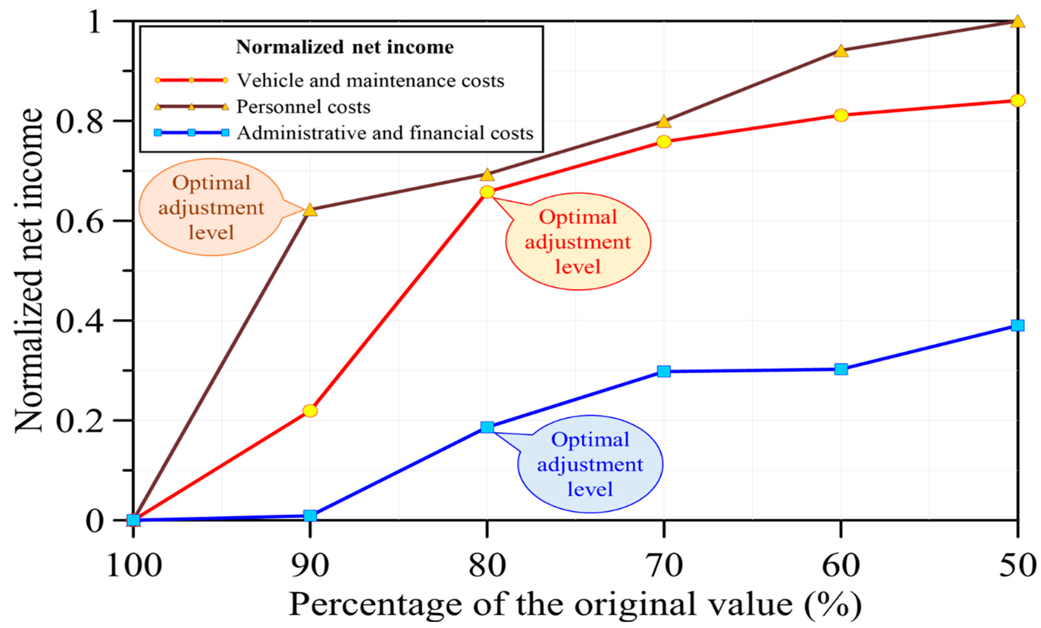
In addition to service frequency, operational costs are also key determinants of net income. Therefore, this study further categorized cost components into three major types: vehicle and maintenance costs, personnel costs, and administrative and financial costs. Proportional reductions of 50%, 60%, 70%, 80%, and 90% were applied to each cost category to simulate and evaluate their respective impacts on net income. The 50–90% cost-reduction scenarios were selected to reflect both phased, practical strategies and more extreme reforms. This range also functions as a sensitivity analysis, illustrating how net income responds to varying cost adjustments and providing decision-makers with a broader perspective on potential policy outcomes.

Figure 9 presents the cost-adjustment net income prediction chart. The x-axis of Figure 9 represents the percentage of the original value, indicating various levels of cost adjustment. Cost adjustments include three major categories: vehicle and maintenance costs, personnel costs, and administrative and financial costs. The percentages range from 100% to 50%, where 100% denotes the original (baseline) cost level, and lower percentages (e.g., 90%) represent cost reductions—such as 90% indicating a 10% decrease in the respective cost category, and so forth. The y-axis of Figure 9 shows the normalized net income, calculated using the following Equation:

$$\mathrm{Normalized} \mathrm{net} \mathrm{income}={\displaystyle \frac{N{I}_x-N{I}_{base}}{N{I}_{\max }-N{I}_{base}}}$$

(12)

where $N{I}_x$ represents the net income corresponding to a specific level of adjustment, $N{I}_{base}$ denotes the total net income of Keelung City’s bus network before adjustment, and $N{I}_{\max }$ denotes the maximum total net income of the bus network observed after adjustment.

According to the analysis results illustrated in Figure 9, the optimal cost-efficiency points for the three cost categories can be identified at specific adjustment levels. For vehicle and maintenance costs, the most favorable outcome is achieved when costs are adjusted to 90% of the original value. For personnel costs, the optimal adjustment level is 80%, yielding the greatest improvement in net income. Similarly, for administrative and financial costs, adjusting to 80% also results in the highest net benefit.

Moreover, personnel costs exhibited the largest marginal effect on net income among all categories. This dominance can be explained from two perspectives: first, personnel expenditures constitute the largest share of the overall cost structure, so any proportional reduction produces a relatively greater absolute financial impact; second, the SVR model shows that net income is more sensitive to changes in personnel costs than in other categories, implying a steeper partial derivative with respect to this variable. The combination of a large baseline magnitude and high response elasticity thus accounts for the strong marginal effect of personnel costs on net income.

In summary, the results demonstrate that service frequency adjustment can effectively optimize operational resource allocation, while cost adjustments, particularly in personnel and vehicle maintenance, significantly contribute to overall revenue enhancement.

6. Discussion

This study applies AI-driven methods, specifically SVR, to predict net revenue and optimize public bus services in Keelung City. The key contributions and limitations of this study are summarized in this Discussion section. The following three key highlights are outlined first:

(1)

In contrast to conventional machine learning (ML) studies that emphasize ridership or fare revenue forecasting, this study develops a predictive framework for route-level net income by explicitly incorporating disaggregated cost components, thereby providing a more rigorous basis for addressing long-term financial sustainability in public bus systems.

(2)

We construct a comprehensive route-level panel dataset integrating 19 operational and financial variables, including service frequency, vehicle-km, and detailed cost categories (personnel, administrative, financial, etc.). In contrast to prior approaches that treat costs implicitly or uniformly, our formulation explicitly encodes heterogeneous cost structures, thereby allowing the estimation of marginal effects by cost type. Additionally, we introduce normalized service frequency and normalized net income to ensure comparability across routes, which is an element typically absent from revenue-only models.

(3)

Beyond predictive accuracy, this study integrates a policy-oriented simulation framework to quantitatively assess the impacts of service and cost adjustments on net income. This approach enables the derivation of operational thresholds applicable to route reallocation and workforce optimization, thereby advancing machine learning applications from purely predictive modeling toward prescriptive, decision-support analysis.

On the other hand, potential limitation of this study is the mileage-based allocation of aggregate cost variables, which may not fully capture route-level cost heterogeneity. While this approach can overstate costs for long, low-ridership routes and understate them for short, high-demand routes, strong correlations between vehicle-kilometers and passenger demand support its validity as a reasonable proxy. Additionally, financial performance is normalized linearly to ensure consistent comparisons across routes, with outlier diagnostics confirming data reliability. Finally, the analysis focuses on financial optimization, without explicitly addressing equity or social impacts, and assumes proportional cost reductions for sensitivity analysis rather than precise operational adjustments.

7. Conclusions

This study introduces an innovative method for optimizing the performance of the public bus services in Keelung City through the application of AI-driven techniques, specifically utilizing SVR for net revenue prediction. The approach significantly enhances the accuracy of revenue forecasting. The key findings of the research are as follows:

(1)

The machine learning model based on SVR was developed, incorporating 19 factors, including vehicle and maintenance costs, personnel costs, administrative and financial costs, and operational data. The SVR model outperformed several other machine learning models, such as RF, ANN, XGBoost, and LightGBM based on comparative analysis. Its predictive performance metrics are as follows: R² = 0.99, RMSE = 5.21 × 10⁻³, VAF = 99.92%, PI = 1.99, MAE = 3.52 × 10⁻³, WI = 0.99, WMAPE = 1.24 × 10⁻², and NS = 0.99. These results indicate that the model is highly accurate and stable, making it suitable for forecasting bus route net revenues.

(2)

Validation of the model was conducted using K-fold cross-validation, which confirmed its strong generalization capabilities and the absence of overfitting. Residual analysis indicated that the distribution of training and test data was consistent, further reinforcing the model’s robustness and its practical applicability.

(3)

Scenario-based simulations evaluated the effects of adjusting service frequency and optimizing cost structures on net income. Results indicate that reducing vehicle and maintenance costs to 90% and personnel as well as administrative and financial costs to 80% yields the most favorable outcomes. Notably, personnel and vehicle maintenance cost reductions offer the greatest revenue gains. Overall, strategic service frequency and targeted cost adjustments can effectively enhance operational efficiency and financial performance, offering practical guidance for improving public transit system profitability.