Modelling the Transition from Shear-Driven Turbulence to Convective Turbulence in a Vertical Heated Pipe

Abstract

Heated pipe flow is widely used in thermal engineering applications, but the presence of buoyancy force can cause intermittency, or multiple flow states at the same parameter values. Such changes in the flow lead to substantial changes in its heat transfer properties and thereby significant changes in the axial temperature gradient. We therefore introduce a model that features a time-dependent background axial temperature gradient, and consider two temperature boundary conditions—fixed temperature difference and fixed boundary heat flux. Direct numerical simulations (DNSs) are based on the pseudo-spectral framework, and good agreement is achieved between present numerical results and experimental results. The code extends Openpipeflow and is available at the website. The effect of the axially periodic domain on flow dynamics and heat transfer is examined, using pipes of length $L=5D$ and $L=25D$. Provided that the flow is fully turbulent, results show close agreement for the mean flow and temperature profiles, and only slight differences in root-mean-square fluctuations. When the flow shows spatial intermittency, heat transfer tends to be overestimated using a short pipe, as shear turbulence fills the domain. This is particularly important when shear turbulence starts to be suppressed at intermediate buoyancy numbers. Finally, at such intermediate buoyancy numbers, we confirm that the decay of localised shear turbulence in the heated pipe flow follows a memoryless process, similar to that in isothermal flow. While isothermal flow then laminarises, convective turbulence in the heated flow can intermittently trigger bursts of shear-like turbulence.

1. Introduction

In the heated flow context, flow driven by an external pressure gradient is referred to as ‘forced’ flow, while buoyancy resulting from the expansivity of the fluid close to a heated wall can provide a force that partially or fully drives the flow, referred to as ‘mixed’ or ‘natural convection’, respectively. In a model, buoyancy may only need to counter drag forces in the vertical pipe. In practice, we are likely to encounter what could be called ‘super-natural’ convection, where the buoyancy must be larger than the local drag in order to drive flow in a wider circuit. In this case, flow in the vertical section of the circuit is subject to a reversed pressure gradient that limits the flow rate.

Turbulent mixed convection in a vertical pipe is a representative model for heat transfer that can be found in thermal engineering applications, e.g., heat exchangers, nuclear reactors, chemical plants and cooling systems for electronic components [1]. Despite the relatively simple geometry, the flow state and heat transfer can be difficult to predict in the presence of buoyancy. Buoyancy can enhance the heat transfer in a heated downward pipe flow but suppress heat transfer in upward heated pipe flow [1,2,3,4,5]. In an upward pipe flow, with the enhancement of heating, heat transfer first deteriorates slowly, then suddenly drops when shear-driven turbulence collapses, then recovers, and finally can approach as large values as for downward flow at large buoyancy parameters [1].

Heat transfer presents some complicated features in upward heated pipe flow, as well as the flow dynamics. Previous research has confirmed three flow states in different heating conditions and Reynolds numbers, i.e., shear turbulence, the laminar state, and convective turbulence [6,7]. The laminar state can persist up to Reynolds numbers of around 3000, versus approximately 2000 in isothermal flow. The addition of buoyancy suppresses and can laminarise shear turbulence. Research on the phenomenon of laminarisation in mixed convection can be traced at least as far back as that of Hall et al. [8], which provided a theoretical explanation of this phenomenon, suggesting that reduced shear stress in the buffer layer leads to a reduction in or even elimination of turbulence production. More recently, He et al. [9] modelled the buoyancy with a radially dependent axial body force added to isothermal flow, successfully reproducing the laminarisation phenomenon. They found that the body force makes little change to the key characteristics of turbulence, and proposed that laminarisation is caused by the reduction in the ‘apparent Reynolds number’, which is calculated based only on the pressure force of the flow (i.e., excluding the contribution of the body force). Similar laminarisation phenomena have also been observed for the isothermal case in the presence of a modified base flow [10,11]. It is conjectured that a flattened velocity profile reduces transient growth [12], thus suppressing shear turbulence. Chu et al. [13] examined the self-sustaining process [14] in this context and found that the flattened velocity profile can suppress the instability of streaks thereby disrupting the self-sustaining process of shear turbulence.

There is a developed history of numerical simulations of mixed convection in vertical pipe flow using various methods. In an early study, a modification of the Redichardt eddy diffusivity model was used to simulate mixed convection [15], but it proved that this approach did not adequately account for certain local features of the flow. Cotton et al. [16] used the low-Reynolds number $k-ϵ$ turbulence model of Lauder et al. [17] to simulate the vertical heated pipe flow with some success. Behzademhr et al. [18] conducted a study of upward mixed convection in a longer pipe at two rather low Reynolds numbers ($Re=1000$ and 1500) over a range of Grashof numbers, which measures the heat flux at the wall, using the Lauder–Sharma model. They identified two critical Grashof numbers for each Reynolds number, which correspond to laminar–turbulent transition and relaminarisation of the flow. More recently, direct numerical simulation (DNS) has been used in studies of mixed convection. Kasagi et al. [19] conducted a DNS study at $Re=4300$ and several values of the Grashof number. The simulations show that buoyancy changes the distribution of Reynolds shear stress and shear production rate of turbulent kinetic energy, leading to heat transfer enhancement or suppression. You et al. [20] also performed the DNS for the mixed convection in vertical pipe flow, and compared the results of upward and downward flow. Kim et al. [21] presented an assessment of the performance of a variety of turbulence models in simulating buoyancy-aided, turbulent mixed convection in vertical pipes. They found the use of different methodologies for modelling the direct production of turbulence through the direct action of buoyancy has been shown to have little effect on predictions of mixed convection in vertical flows. Chu et al. [22] applied a well-resolved DNS to investigate strongly heated airflow in a vertical pipe at $Re=4240$ and 6020. The results showed excellent agreement in heat transfer and flow statistics. Recent calculations at larger flow rates include [23,24,25].

We wish to examine the detailed transient nature of transition, for which accurate DNS is necessary, and since the flow type ultimately affects the heat transfer and hence the heating of the fluid itself, we wish to explicitly include a time-dependent temperature gradient. The model developed by Marensi et al. [6] extends the pseudo-spectral code openpipeflow [26] to include a time-dependent spatially uniform heat sink. This form for the sink has the advantage of a simple analytic expression for the laminar state. Numerical results showed good agreement with the experimental results but were improved slightly by Chu et al. [7] by associating the heat sink with a time-dependent background temperature gradient along the axis of the pipe. In both Marensi et al.’s [6] and Chu et al.’s [7] works, fixed temperature conditions were used at the wall. In this work, we provide further details of the model of Chu et al. [7] and add a second case for the temperature boundary condition, that of fixed heat flux at the wall.

It should be noted that our model assumes axial periodicity, which implies that it should be applied to a straight section of pipe, downstream of the effects from an inlet or bend. This approximation is widely adopted for research in shear turbulence [27,28] and mixed convection [25] in pipe flows. Another potential limitation is the Boussinesq approximation [29,30] adopted in our model, which ignores the effect of heating on viscosity and assumes that changes of density only need be considered in the buoyancy force term in Navier–Stokes equations. Nevertheless, such modelling simplifies the simulation greatly and provides good results in many circumstances [29], and has been widely adopted in the simulations of mixed convection [20,25,31]. As we focus on flow and heating rates that are transitional with respect to flow regimes, we do not consider extreme parameter values here. When the Boussinesq approximation holds, there is mathematical equivalence between upward heated and downward cooled flow, i.e., the case modelled here could be experimentally examined by considering a hot fluid flowing down a pipe through a cold room. Although the temperature along the pipe will approach the room temperature exponentially under such circumstances, it can be modelled to be locally linear over a reasonable distance, and the temperature gradient along the pipe will depend on whether the flow is laminar or turbulent. Finally, it should also be noted that turbulence increases friction drag and hence pumping costs. The relative importance of this cost is very context specific, and therefore is not considered here. Our focus is on the enhanced heat transfer due to turbulence.

The plan of the paper is as follows. In Section 2, we present the model for the DNS of vertical heated pipe flow, including two types of temperature boundary conditions, i.e., fixed temperature difference and fixed boundary heat flux. In Section 3, we first show the results of DNS, then present the results of different lengths of pipe. Next, we show how the lifetime of shear turbulence changes with buoyancy force. Finally, the paper concludes with a summary in Section 4.

2. Model for Heated Pipe Flow

Let $\mathit{x}=(r,\varphi ,z)$ denote cylindrical coordinates within a pipe of radius R. The total temperature satisfies

$${\displaystyle \frac{\partial T_{tot}}{\partial t}}+({\mathit{u}}_{tot}·\nabla )T_{tot}=\kappa {\nabla }^2{T}_{tot},$$

(1)

where $\kappa$ is the thermal diffusivity. We decompose the total temperature as

$$\begin{array}{ccc}\hfill T_{tot}(\mathit{x},t)& =& T_w(z,t)+T(\mathit{x},t)-T_0,\hfill \end{array}$$

(2)

$$\begin{array}{ccc}\hfill T_w(z,t)& =& a\left(t\right)z+b,\hfill \end{array}$$

(3)

where $a\left(t\right)$ is the time-dependent axial temperature gradient, b is a constant reference temperature, $T(\mathit{x},t)$ carries the temperature fluctuations, and $T_0$ is a constant that will be used as a temperature scale. The factor $-T_0$ is inserted in (2) so that the temperature fluctuations T are positive and largest at the hot wall. The bulk temperature, we write as

$$T_b=⟨T⟩,$$

(4)

where the angle brackets denote the volume average. The important quantity that measures the heat flux is the Nusselt number

$$\mathit{Nu}={\displaystyle \frac{2R{q}_w}{\lambda \left({T|}_{r=R}-T_b\right)}}.$$

(5)

where $\lambda$ is the thermal conductivity, and $q_w=\lambda \overline{{(\partial T/\partial r)|}_{r=R}}$ is the heat flux at the wall, where the overline denotes the time average. Note that $\mathit{Nu}$ is an observed quantity, rather than a prescribed parameter, as it depends on the state of the flow.

For the fixed temperature boundary condition, $T_w$ is the value of the temperature at the wall. Evaluating (2) at the wall gives ${T|}_{r=R}=T_0$. The wall temperature is locally isothermal (does not deviate from $T_w$), while the heat flux may exhibit variations. However, $q_w$ can be measured and is expected to be statistically steady, except when interrupted by a change in state of the flow, such as from shear turbulence to convective turbulence.

For the fixed heat-flux boundary condition, $q_w$ takes the same value everywhere. Local variations in the boundary temperature are possible, so that here, $T_w$ represents an averaged wall temperature. Note that $\mathit{Nu}$ will still vary through changes in $T_b$.

Throughout the rest of this work, dimensionless variables and equations are presented, except in the definition of the scales and dimensionless parameters. We use R as the length scale and twice the bulk flow speed $2U_b$ for the velocity scale, which for isothermal laminar flow coincides with the centreline speed. For the temperature scale, we use $T_0$, which will be linked to the boundary conditions in the following sections. Using these scales, we arrive at the dimensionless governing equation

$${\displaystyle \frac{\partial T}{\partial t}}+({\mathit{u}}_{tot}·\nabla )T={\displaystyle \frac{1}{RePr}}{\nabla }^{2}T-{\mathit{u}}_{tot}·\widehat{\mathit{z}}a\left(t\right),$$

(6)

where it is assumed that variations in the temperature gradient are much slower than variations in the local fluctuations, i.e., ${\partial }_{t}a\left(t\right)\ll {\partial }_{t}T(\mathit{x},t)$. The dimensionless parameters are the Reynolds and Prandtl numbers $Re=2U_{b}R/\nu$ and $Pr=\nu /\kappa$, where $\nu$ and $\kappa$ are the kinematic viscosity and thermal diffusivity. A Prandtl number of 0.7 is used in all calculations. The last term on the right-hand side is a sink term that withdraws the energy that enters through the boundary. The value for $a\left(t\right)$ at each instant is determined via the spatial average of (6) and depends on the boundary condition on the temperature as shown in the following sections. Axial periodicity over a dimensionless distance $L=2\pi /\alpha$ is assumed for the temperature fluctuation field $T(\mathit{x},t)$.

Axial periodicity is also assumed for the velocity field ${\mathit{u}}_{tot}(\mathit{x},t)$. Under the Boussinesq approximation [30], the dimensionless Navier–Stokes (NS) equations are

$${\displaystyle \frac{\partial {\mathit{u}}_{tot}}{\partial t}}+({\mathit{u}}_{tot}·\nabla ){\mathit{u}}_{tot}=-\nabla p+{\displaystyle \frac{1}{Re}}{\nabla }^2{\mathit{u}}_{tot}+{\displaystyle \frac{\gamma gR{T}_0}{{\left(2U_b\right)}^2}}T\widehat{\mathit{z}}+{\displaystyle \frac{4}{Re}}(1+\beta \left(t\right))\widehat{\mathit{z}},$$

(7)

with continuity equation

$$\nabla ·{\mathit{u}}_{tot}=0,$$

(8)

and no-slip condition ${\mathit{u}}_{\mathit{tot}}=\mathbf{0}$ at the wall, where $\gamma$ is the thermal expansivity and g is acceleration due to gravity. Here, $⟨{\partial }_{z}p⟩=0$, and the non-zero component of the axial pressure gradient appears in the final term of (7); $\beta \left(t\right)$ is the excess pressure fraction, relative to isothermal laminar flow, required to maintain the fixed dimensionless mass flux $⟨{\mathit{u}}_{tot}·\widehat{\mathit{z}}⟩=1/2$. Further decomposing the variables as

$$\begin{array}{ccc}\hfill {\mathit{u}}_{tot}(\mathit{x},t)& =& u_0\left(r\right)\widehat{\mathit{z}}+\mathit{u}(\mathit{x},t),u_0=1-r^2,\hfill \end{array}$$

(9)

$$\begin{array}{ccc}\hfill T(\mathit{x},t)& =& {\Theta }_0\left(r\right)+\Theta (\mathit{x},t),{\Theta }_0=r^2,\hfill \end{array}$$

(10)

leads to governing equations for the deviation fields $\Theta$ and $\mathit{u}=(u_r,u_{\varphi },u_z)$

$$\begin{array}{c}\hfill {\displaystyle \frac{\partial \Theta }{\partial t}}+u_0{\displaystyle \frac{\partial \Theta }{\partial z}}+u_r{\displaystyle \frac{d{\Theta }_0}{dr}}+(\mathit{u}·\nabla )\Theta ={\displaystyle \frac{1}{RePr}}{\nabla }^2\Theta +{\displaystyle \frac{4}{RePr}}-(u_0+u_z)a\left(t\right),\end{array}$$

(11)

$$\begin{array}{c}\hfill {\displaystyle \frac{\partial \mathit{u}}{\partial t}}+u_0{\displaystyle \frac{\partial \mathit{u}}{\partial z}}+u_r{\displaystyle \frac{d{u}_0}{dr}}\widehat{\mathit{z}}+(\mathit{u}·\nabla )\mathit{u}=-\nabla p+{\displaystyle \frac{1}{Re}}{\nabla }^2\mathit{u}+{\displaystyle \frac{4}{Re}}(C(\Theta +{\Theta }_0)+\beta \left(t\right))\widehat{\mathit{z}},\end{array}$$

(12)

with continuity condition $\nabla ·\mathit{u}=0$ and boundary condition $\mathit{u}=\mathbf{0}$. The parameter C measures the buoyancy force relative to the pressure gradient for laminar flow. Equating buoyancy terms in (7) and (12), we have

$${\displaystyle \frac{4}{Re}}C={\displaystyle \frac{\gamma gR{T}_0}{{\left(2U_b\right)}^2}},$$

(13)

where $T_0$ will be specified according to the boundary condition on $\Theta$. To determine $\beta \left(t\right)$, we take the spatial average of the z-component of (12). By Gauss’s theorem and the divergence-free condition, many terms drop. Noting also that $⟨u_0⟩=⟨{\Theta }_0⟩=1/2$, the $\beta \left(t\right)$ that fixes $⟨u_z⟩=0$ is given by

$$\beta \left(t\right)=-C\left({\displaystyle \frac{1}{2}}+⟨\Theta ⟩\right)-{\displaystyle \frac{1}{2}}{\left.{\displaystyle \frac{\partial {\left(u_z\right)}_{00}}{\partial r}}\right|}_{r=1},$$

(14)

where ${(·)}_{00}$ denotes averaging over $\varphi$ and z.

2.1. Fixed Temperature Difference Between Bulk and Boundary

We accompany the fixed temperature boundary condition with a fixed bulk temperature $T_b$ in (4). Making the choice

$$T_0=2T_b$$

(15)

for the temperature scale, inserting in (13) and rearranging, we find

$$C_{\Delta T}={\displaystyle \frac{G{r}_{\Delta T}}{16Re}},G{r}_{\Delta T}={\displaystyle \frac{\gamma g(T{|}_{r=R}-T_b){\left(2R\right)}^3}{{\nu }^2}}$$

(16)

wherein we use the dimensional T of (2) and subscript the parameters to clarify that they are based on a temperature difference. $G{r}_{\Delta T}$ is the Grashof number.

Using the scale $T_0=2T_b$ to non-dimensionalise (2) and (4), the dimensionless fluctuations satisfy ${T|}_{r=1}=1$ and $⟨T⟩=1/2$. As a simple ${\Theta }_0$ is chosen that satisfies these conditions, we have that (11) is accompanied by the boundary condition ${\Theta |}_{r=1}=0$ and the condition $⟨\Theta ⟩=0$. The latter condition is equivalent to saying that the energy within the domain is constant, and hence the energy entering the domain through the boundary must match the energy extracted by the sink term at each instant. This sets a value for $a\left(t\right)$. Taking the spatial average of (11) gives

$$a\left(t\right)={\displaystyle \frac{4}{RePr}}\left(2+{\left.{\displaystyle \frac{\partial {(\Theta )}_{00}}{\partial r}}\right|}_{r=1}\right).$$

(17)

This model was applied in the simulations of Chu et al. [7].

2.2. Fixed Heat Flux at the Boundary

As we already have that $\left({\partial }_r{\Theta }_0\right){|}_{r=1}=2$ in the decomposition (10), we suppose that this is the value of the temperature gradient everywhere, and accompany (11) with the boundary condition $({\partial }_r\Theta ){|}_{r=1}=0$. Using $T_0$ as the temperature scale, the dimensional flux at the wall is everywhere

$$q_w=2\lambda {\displaystyle \frac{T_0}{R}},\text{i.e.,}{T}_0={\displaystyle \frac{q_{w}R}{2\lambda }}.$$

(18)

Inserting this $T_0$ in (13) and rearranging, we find

$$C_q={\displaystyle \frac{G{r}_q}{128Re}},G{r}_q={\displaystyle \frac{\gamma g{\left(2R\right)}^4{q}_w}{\lambda {\nu }^2}},$$

(19)

where the subscripts are added to the parameters to indicate that they are based on the heat flux.

The fluctuations may be split into a spatial mean and varying component, $\Theta (\mathit{x},t)={(\Theta )}_{00}(r,t)+{\Theta }^{\prime }(\mathit{x},t)$, where ${(·)}_{00}$ denotes averaging over $\varphi$ and z. To the varying components, we apply the boundary condition $\left({\partial }_r{\Theta }^{\prime }\right){|}_{r=1}=0$. The mean component evolves according to the spatial average of (11), which may be written

$${\displaystyle \frac{\partial {(\Theta )}_{00}}{\partial t}}-{\displaystyle \frac{1}{RePr}}{\nabla }^2{(\Theta )}_{00}={\left(N\right)}_{00}-(u_0+{\left(u_z\right)}_{00})a\left(t\right).$$

(20)

We wish the mean component to be consistent with there being a constant background reference temperature in (3), and therefore apply the boundary condition ${(\Theta )}_{00}{|}_{r=1}=0$. Note that the temperature can still vary at the boundary, as this condition only fixes the mean value. However, it still remains to apply the boundary condition $\left({\partial }_r{(\Theta )}_{00}\right){|}_{r=1}=0$, which is achieved through the variation in $a\left(t\right)$. Evaluating the radial derivative at the wall gives

$$a\left(t\right)={\left.\left({\displaystyle \frac{\partial {\left(N\right)}_{00}}{\partial r}}+{\displaystyle \frac{1}{RePr}}{\displaystyle \frac{\partial {\nabla }^2{(\Theta )}_{00}}{\partial r}}\right)\right|}_{r=1}/{\left.\left(-2+{\displaystyle \frac{\partial {\left(u_z\right)}_{00}}{\partial r}}\right)\right|}_{r=1}.$$

(21)

It is worth mentioning that accompanying (11) with the condition $({\partial }_r\Theta ){|}_{r=1}=0$ alone, the problem is ill-posed; see [32,33]. The condition ${(\Theta )}_{00}{|}_{r=1}=0$ removes non-uniqueness, but note that it cannot be trivially satisfied by evaluating (20) at the wall—$a\left(t\right)$ remains undetermined, as its coefficient is zero at the wall.

2.3. Time-Integration Code

The calculations are carried out by the open-source code openpipeflow.org (accessed on 15 March 2024) [26]. Variables are discretised on the domain $\left\{r,\varphi ,z\right\}=[0,1]\times [0,2\pi ]\times [0,2\pi /\alpha ]$, where $\alpha =2\pi /L$, using Fourier decomposition in the azimuthal and streamwise directions and finite difference in the radial direction, with points clustered towards the wall. An arbitrary variable $f\left(\mathit{x}\right)$ is expanded in the form

$$f(r_s,\varphi ,z)=\sum _{k<\left|K\right|}\sum _{m<\left|M\right|}{\left(f\right)}_{km}\left(r_s\right)e^{i(\alpha kz+m\varphi )},s=1,2,\cdots ,S,$$

(22)

and the mode ${\left(f\right)}_{00}$ corresponds to the $\varphi$- and z-average. Temporal discretisation is via a second-order predictor-corrector scheme, with an Euler predictor and a Crank–Nicolson corrector applied to the nonlinear terms. The laminar solution is quickly calculated by eliminating azimuthal and axial variations using a resolution $S=64,M=1,K=1$. For a periodic pipe of length $L=5D$, the resolution is $S=64,M=76,K=80$ at $Re=5300$, and the resolution is $S=64,M=40,K=44$ at $Re=3000$. For a periodic pipe of length $L=25D$, the resolution is $S=64,M=76,K=400$ at $Re=5300$, and the resolution is $S=64,M=40,K=220$ at $Re=3000$. A time step of $\Delta t=0.01$ is adopted. These resolutions ensure a drop-off of three to four orders of magnitude in the amplitude of the spectral coefficients, which experience has shown to be sufficient for accurately simulating shear-turbulence, matching the statistics from, for example, [27]. Within the parameter range considered here, the convective state is less computationally demanding to simulate.

3. Results

In this section, we compare the two different boundary conditions keeping $L=5D$, then we consider the fixed temperature difference boundary condition and compare the flow in $L=5D$ and $L=25D$. Finally, we calculate the heat transfer and lifetimes for localised turbulence in the presence of the buoyancy force.

3.1. Laminar Flow, Shear Turbulence and Convective Turbulence

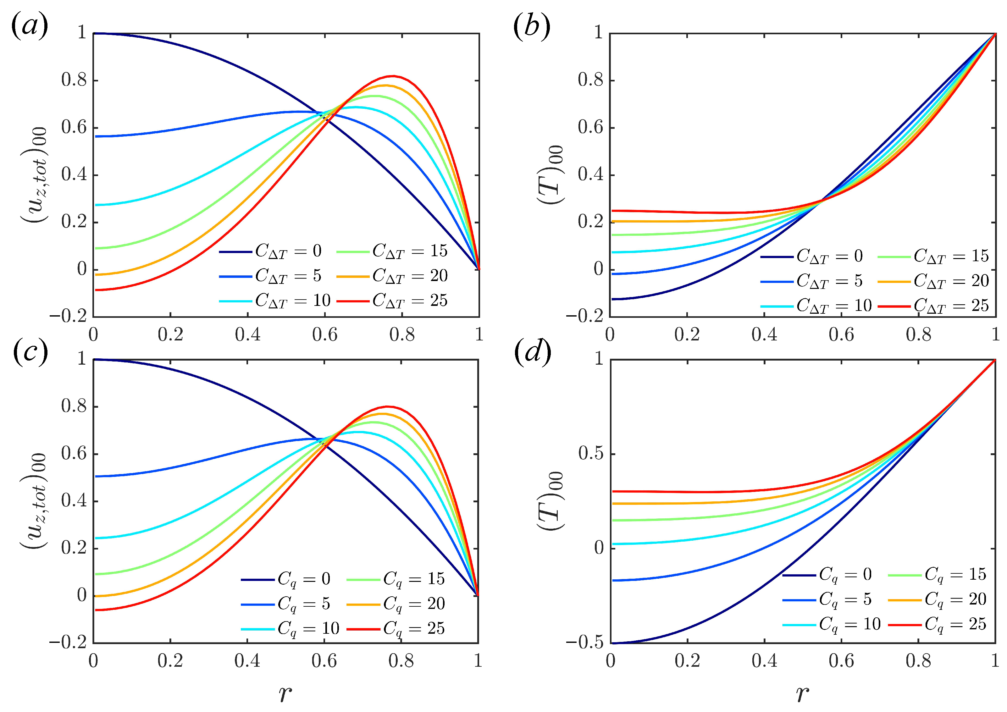
We first verify that the model produces the well-known properties of the laminar solution for both models and for increasing buoyancy parameter C [31,34], shown in Figure 1. The results in Figure 1 are calculated at $Re=5300$, but laminar profiles are dependent on C and independent of $Re$ [31]. The laminar velocity profile becomes flattened and even ‘M’ shaped with the enhancement of heating. Negative velocity near the centre of the pipe at $C_{\Delta T},C_q=20,25$ indicates the occurrence of reversed flow. The laminar temperature profile becomes flattened as C increases. For the fixed temperature difference, an increased temperature gradient near the wall implies increased heat flux and increased Nusselt number $\mathit{Nu}$, defined in (5). For the fixed heat flux case, a reduced temperature difference between the wall and bulk results in increased $\mathit{Nu}$.

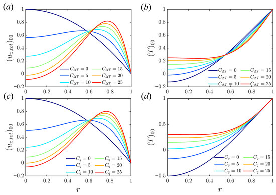
Figure 1. Laminar solution for (a,b) fixed temperature difference; (c,d) fixed boundary heat flux.

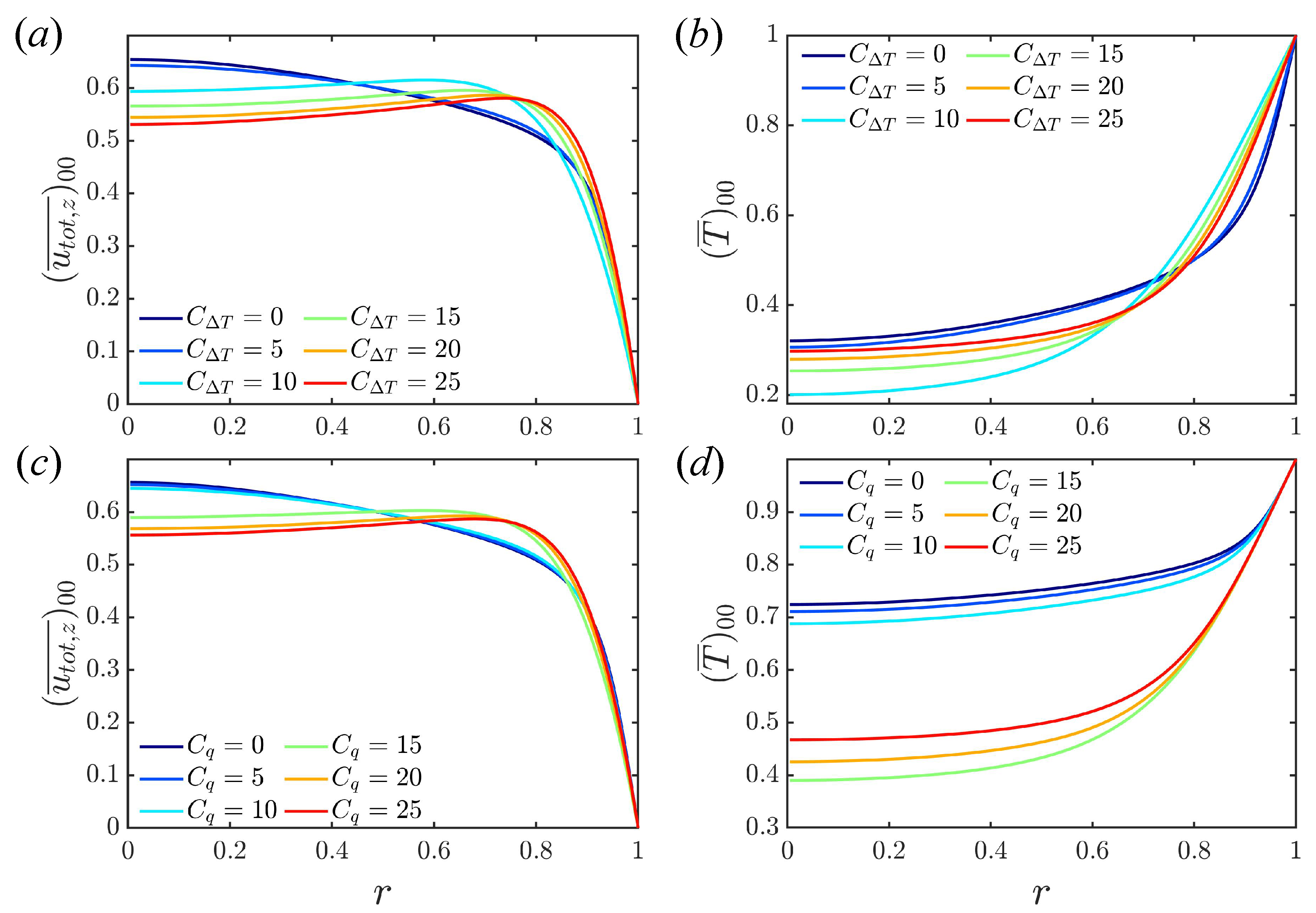
Turbulent mean profiles at $Re=5300$ are shown in Figure 2. Two regimes are observed in both the velocity and temperature profiles, corresponding to shear-driven turbulence and convective turbulence. For the velocity profile, the former state has a flattened shape, while the latter has an ‘M’ shape due to the stronger influence of the buoyancy force. For these values of C, shear turbulence has much greater heat transfer than convective turbulence. As C increases, it is observed that heat transfer first becomes weaker, then collapses, and finally, it gradually recovers. This trend is consistent with the results reported in the literature [1,20,35,36,37]. Both models capture a similar change in heat transfer but with different critical values of the C parameters.

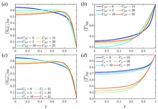
Figure 2. Turbulent mean velocity profiles $\overline{u_{tot,z}}$ and temperature profiles $\overline{T}$ at $Re=5300,L=5D$: (a,b) fixed temperature difference; (c,d) fixed boundary heat flux.

Numerical results for the present model are compared with the previous numerical results [6,20] and experimental results [35,36,37], shown in Figure 3 (Fixed temperature difference and uniform heat sink were adopted by Marensi et al. [6], while fixed heat flux was applied by You et al. [20]). Averages over at least 4000 time units are used in the calculation of $\mathit{Nu}$. Two regimes are clearly identified, i.e., the heat-transfer deterioration regime and the recovery regime, corresponding to shear turbulence and convective turbulence, respectively. Both temperature boundary conditions achieve good agreement with the experimental results and previous numerical results.

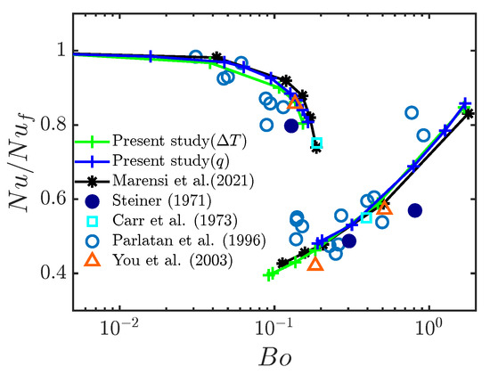
Figure 3. Change in heat flux, normalised by that for the isothermal state ($C\to 0$), as a function of $Bo=8\times {10}^4\left(8\mathit{Nu}G{r}_{\Delta T}\right)/\left(R{e}^{3.425}P{r}^{0.8}\right)$ (fixed temperature difference) or $Bo=8\times {10}^4\left(8G{r}_q\right)/\left(R{e}^{3.425}P{r}^{0.8}\right)$ (fixed boundary heat flux). Present data from simulations at $Re=5300$, $Pr=0.7$. The upper and lower branches correspond to shear and convective turbulence, respectively. Data from [6,20,35,36,37].

At lower Reynolds numbers, there is a laminarisation regime, seen in Figure 4, which shows the approximate regions of the flow states for the two temperature boundary conditions. Although there is a difference between the values of $C_{\Delta T}$ and $C_q$ at which transition between different flow regimes occurs, they are consistent in Figure 3.

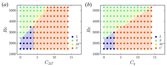
Figure 4. Approximate regions of laminar flow (L), shear turbulence (S), and convective turbulence (C); SC indicates that the flow may be in either of the two states. (a) Fixed temperature difference; (b) fixed boundary heat flux.

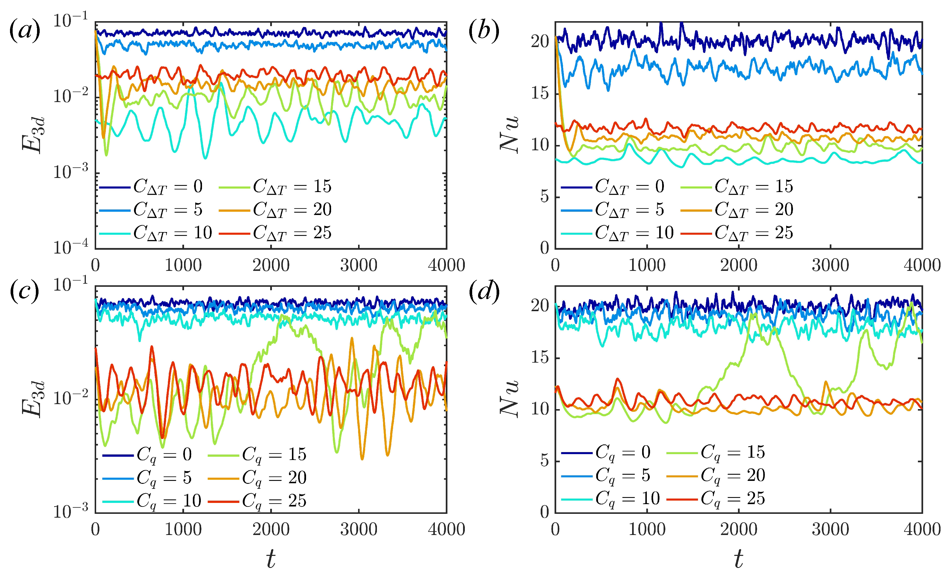
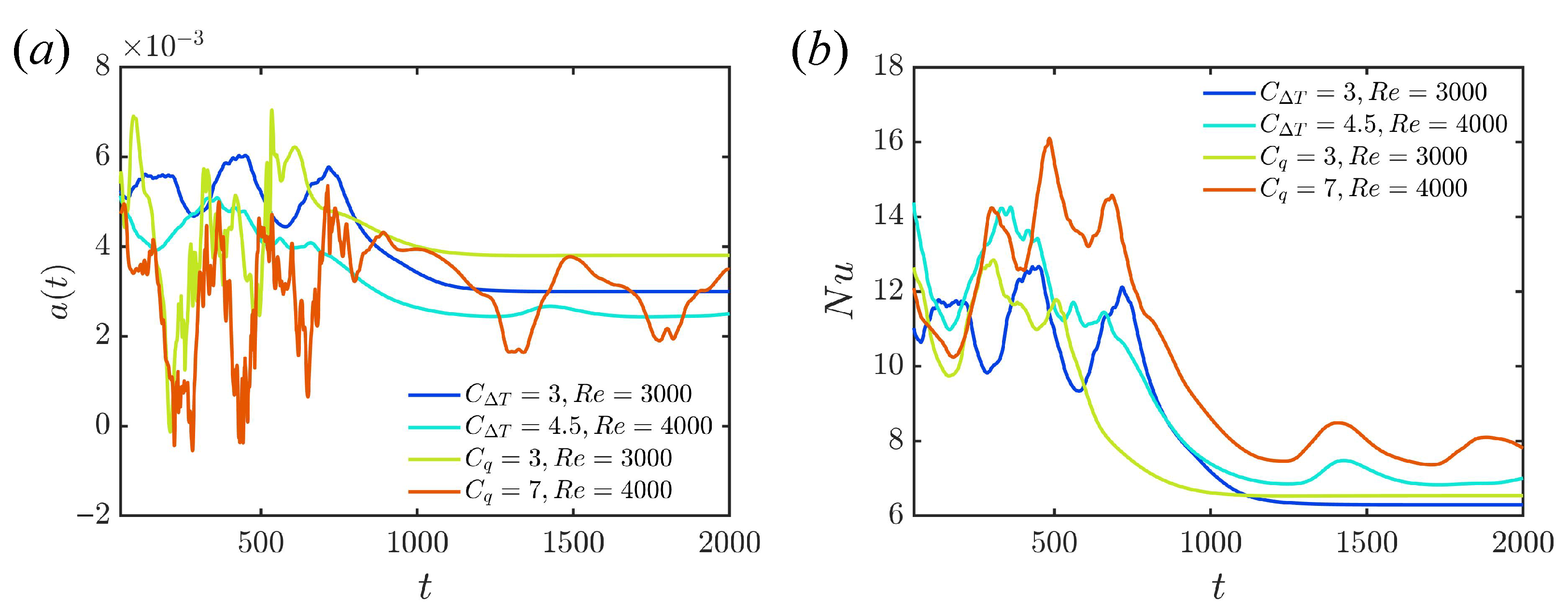
The time evolution of $E_{3d}$ (energy of streamwise-dependent component of the flow) and instantaneous $\mathit{Nu}\left(t\right)$ at different $C_{\Delta T}$ and $C_q$ are presented in Figure 5. Generally, as C is increased, $E_{3d}$ first decreases gradually, then reduces to a much lower energy level at a critical value of C, indicating a flow state transition from shear turbulence to convective turbulence [7]. In the convective turbulence state, $E_{3d}$ fluctuates with a much lower frequency. A clear gap between the shear turbulence regime and the convective turbulence regime (smaller $E_{3d}$ and $\mathit{Nu}$) is observed. The critical C is not precise, since close to the border, both states can be observed. At $Re=5300$, the critical values are $C_{\Delta T}\approx 7$ and $C_q\approx 15$. Interestingly, bistability is observed at $C_q=15$, which switches between shear and convective turbulence. In particular, the convective state is capable of intermittently triggering bursts of shear-like turbulence, whereas at lower $Re$ and in isothermal flow, it cannot switch back from the linearly stable laminar state.

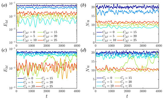
Figure 5. (a,c) Time series of $E_{3d}$ (energy of the streamwise-dependent component of the flow) and (b,d) $\mathit{Nu}\left(t\right)$ at different $C_{\Delta T}$ and $C_q$ for $Re=5300$.

The time evolutions of the background temperature gradient $a\left(t\right)$ and of $\mathit{Nu}\left(t\right)$ are presented in Figure 6 during the transition from shear turbulence to the laminar state, and during the transition from shear turbulence to convective turbulence for the two types of boundary conditions. The transition from shear turbulence to either the laminar state or convective turbulence leads to a reduced Nusselt number. This is accompanied by a reduction in the gradient $a\left(t\right)$ for the fixed temperature difference model. As the heat transfer associated with the new flow is lower, the fluid is heated less, and the gradient reduces. For the fixed heat flux model, however, once the total temperature has adjusted (giving the change in $\mathit{Nu}$), the time average of $a\left(t\right)$ is forced to remain the same so that the heat flux out matches the fixed input flux. As the energy of the bulk is fixed for the fixed temperature difference, the input and output energies respond immediately to each other, so that $a\left(t\right)$ and $\mathit{Nu}\left(t\right)$ vary together. For the fixed flux condition, $\mathit{Nu}\left(t\right)$ varies due to differences in the bulk temperature, which responds in a time-integrated fashion relative to the heat flux out. Hence, fluctuations in $\mathit{Nu}\left(t\right)$ are less rapid than those in $a\left(t\right)$ for the fixed flux boundary condition.

Figure 6. Time evolution of (a) $a\left(t\right)$ and (b) instantaneous Nusselt number when shear turbulence collapses to the laminar or convective state for the two boundary conditions.

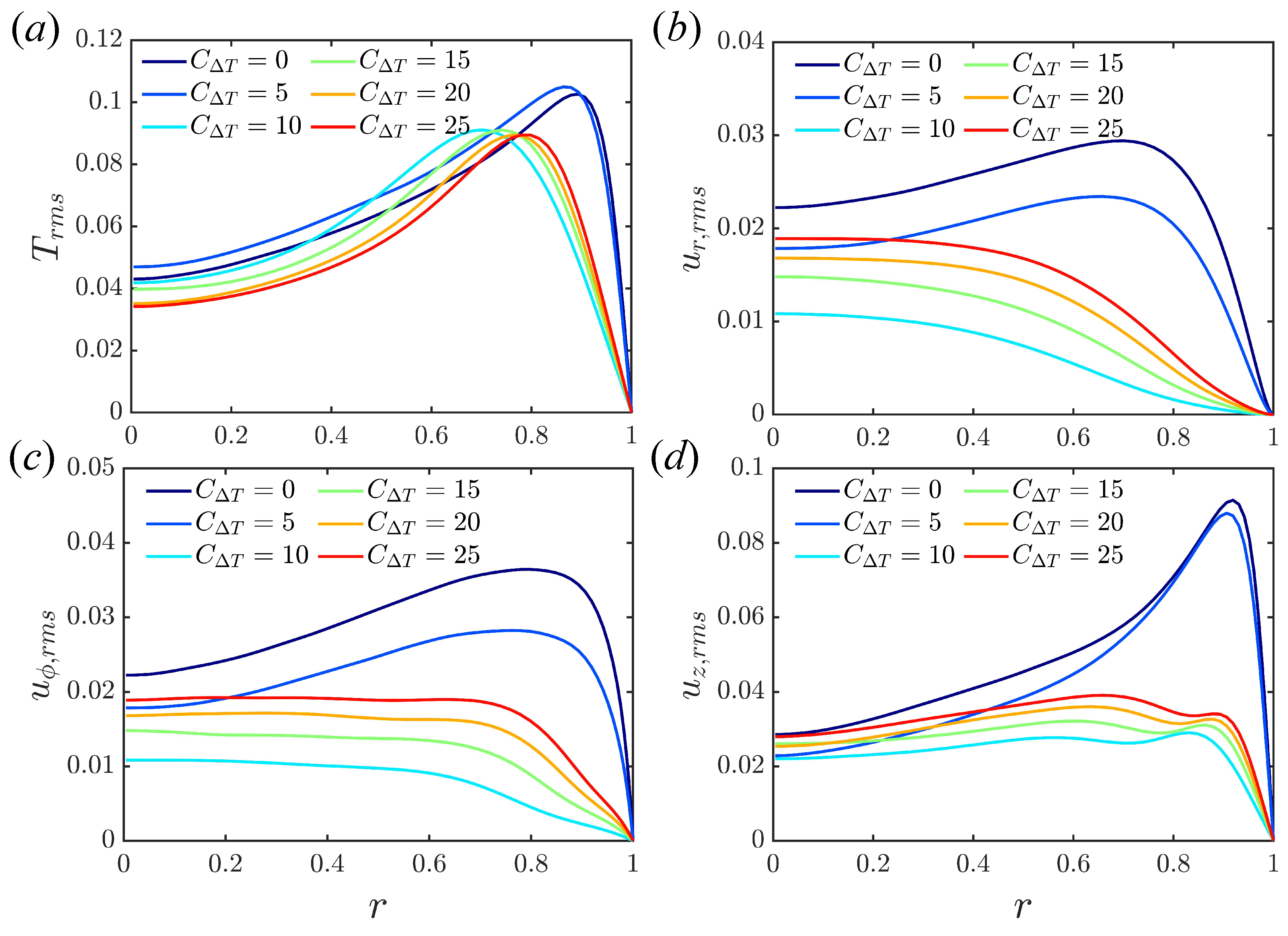
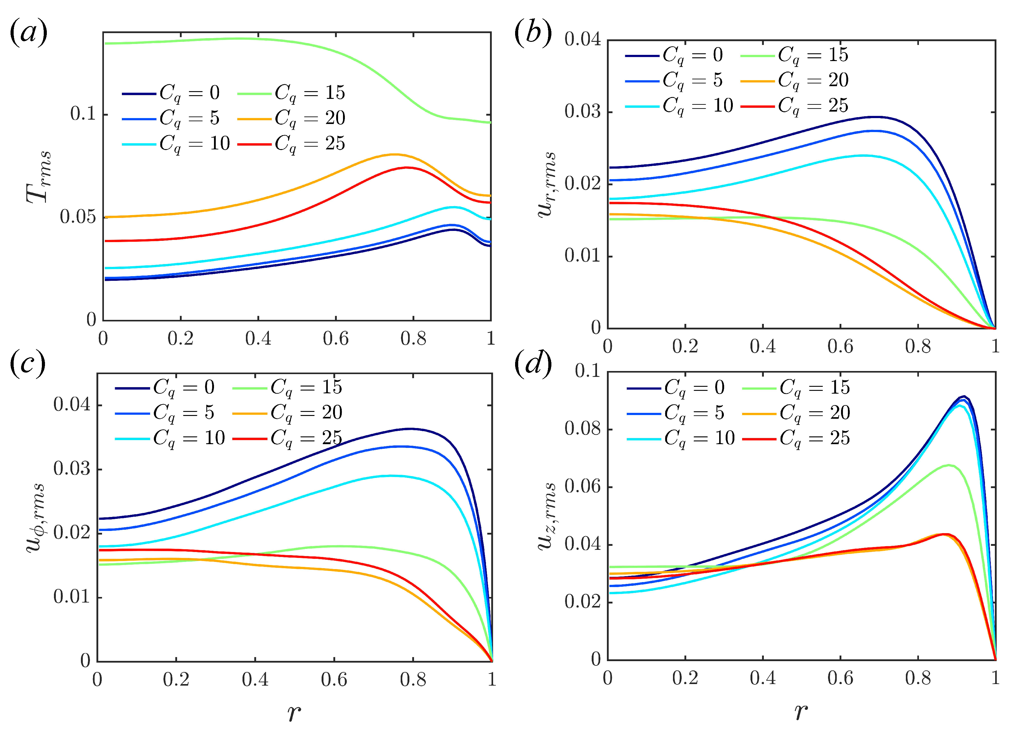
Root-mean-square (RMS) deviations from $\overline{{\left(u_{z,tot}\right)}_{00}}$ and $\overline{{\left(T\right)}_{00}}$ are shown in Figure 7 and Figure 8 for the fixed temperature and fixed flux boundary conditions, respectively, using data from $t=1000$ to $t=4000$ for each simulation. Interestingly, there are two peaks of streamwise velocity fluctuation observed in convective turbulence when the fixed temperature difference is adopted; see Figure 7d. At $C_{\Delta T}=10$, the peak near the wall dominates, while the peak far away from the wall is larger at $C_{\Delta T}=25$. The two peaks are in good agreement with You et al. [20] in Figure 4 and Cruz et al. [25] in Figure 3. The main difference between the two models is in the temperature fluctuations $T_{rms}$. As only the mean temperature at the wall is fixed for the fixed flux model, fluctuations are possible even at the wall. $T_{rms}$ for $C_q=15$ is especially large, due to the bistability mentioned earlier (see Figure 5c,d). Otherwise, the results are similar, and differences between the shear and convective regimes are observed in the RMS fluctuations for both models. In the shear turbulence regime, the peak of temperature fluctuation is close to the wall and moves away from the wall with increased heating. In the convective turbulence regime, the peak of the temperature fluctuations is much further away from the wall, and moves closer to the wall again as the heating is increased. The peak fluctuations for all velocity components are close to the wall in the shear turbulence regime, and weaken as C increases. For the convective regime, fluctuations are spread more evenly across the domain and strengthen as C increases further. Results are consistent with other calculations of RMS quantities [20,25,38].

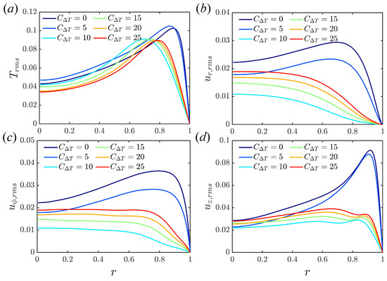
Figure 7. Profiles of RMS temperature and velocity fluctuations at $Re=5300,L=5D$: (a) $T_{rms}$; (b) $u_{r,rms}$; (c) $u_{\varphi ,rms}$; (d) $u_{z,rms}$. Fixed temperature difference.

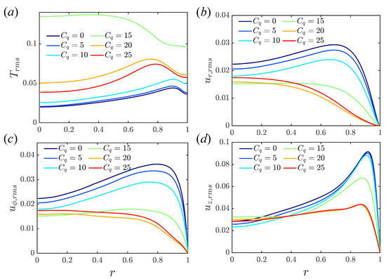
Figure 8. The profile of root mean square of temperature and velocity at $Re=5300,L=5D$: (a) $T_{rms}$; (b) $u_{r,rms}$; (c) $u_{\varphi ,rms}$; (d) $u_{z,rms}$. Fixed boundary heat flux.

3.2. Short vs. Long Periodic Pipes

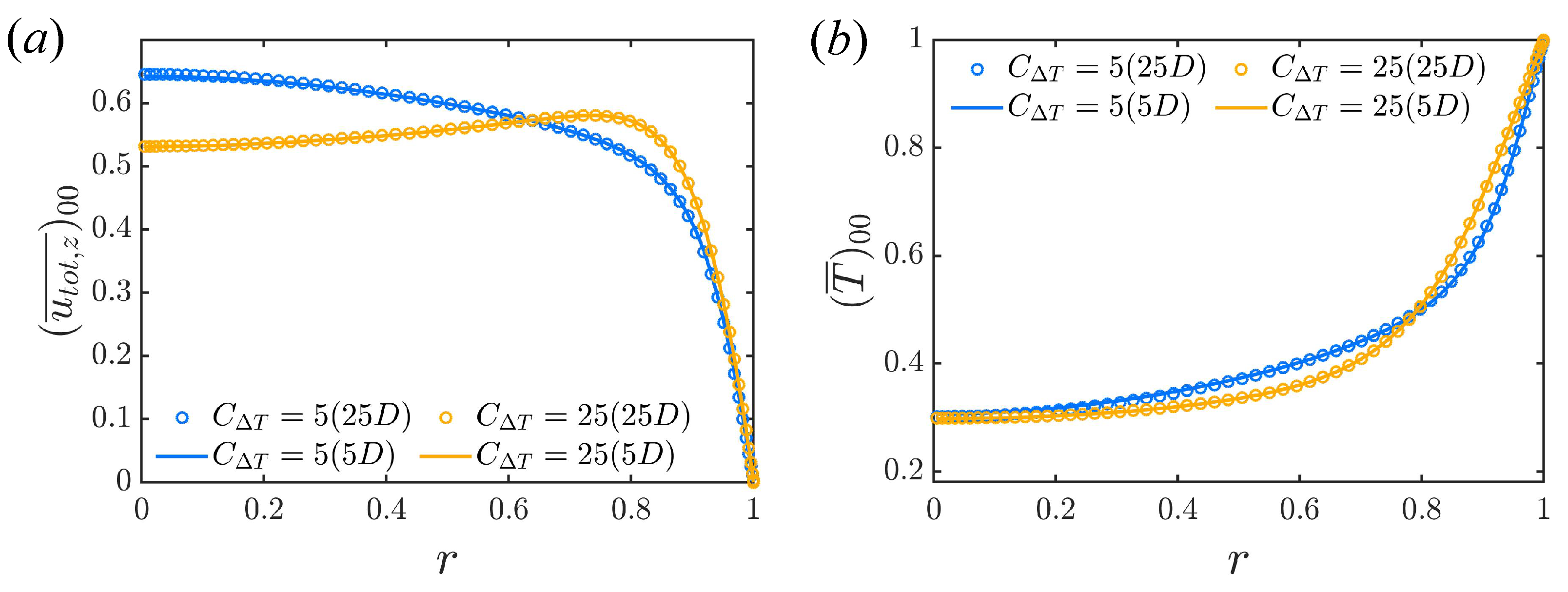
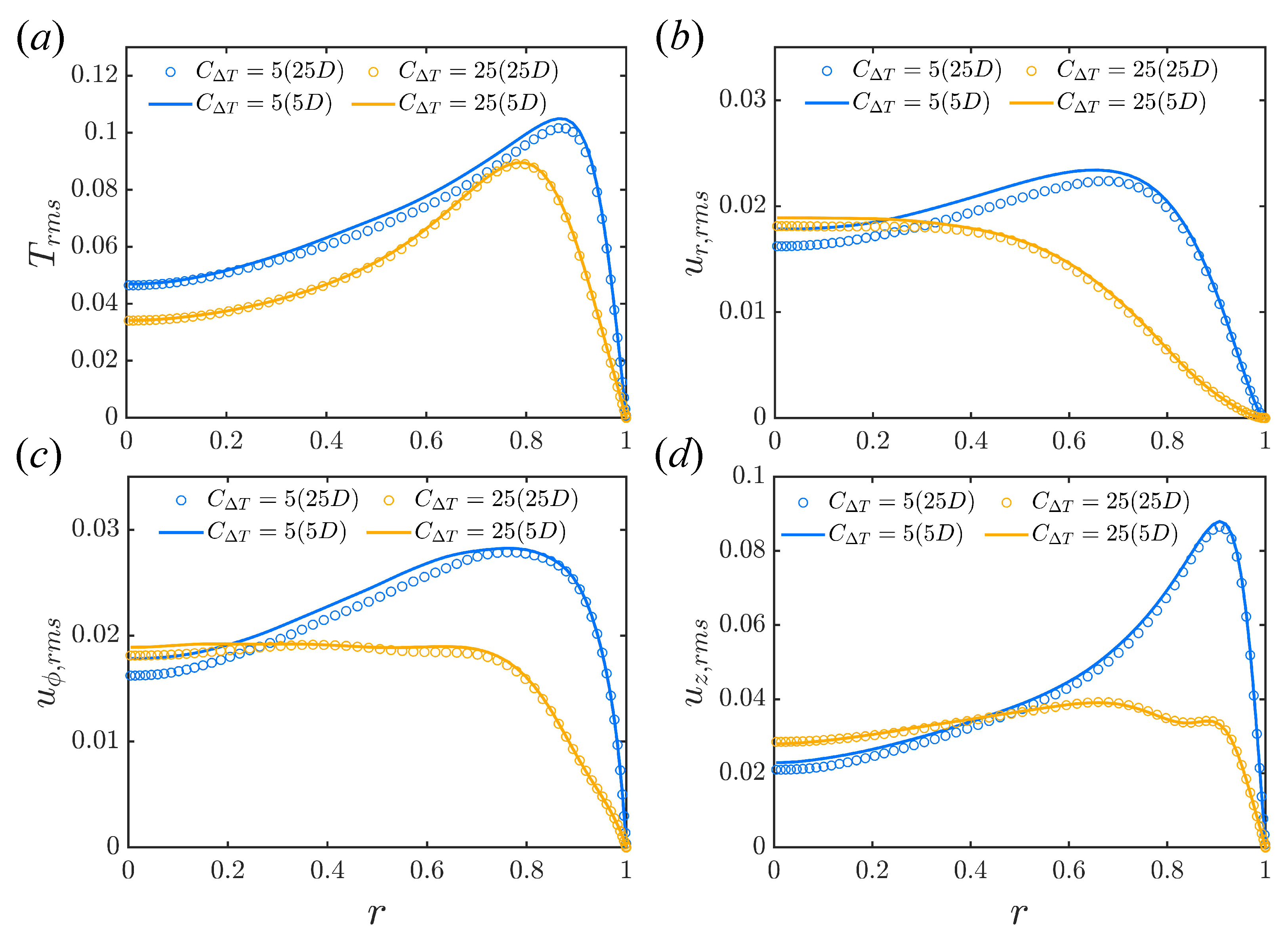
As the two models give consistent results, only the fixed temperature difference model is considered here. The axially periodic boundary condition could impose some difference in the results compared to true flow. Thus, here we use a longer pipe, $L=25D$, for comparison. Figure 9 shows the mean velocity and temperature profiles of a short pipe ($L=5D$) and a longer pipe ($L=25D$) in shear turbulence regime ($C_{\Delta T}=5$) and strong convective turbulence ($C_{\Delta T}=25$). The results for the two pipe lengths are in good agreement, suggesting that $L=5D$ is enough for capturing the mean profiles. The distributions of the RMS of temperature and velocity for the short pipe and long pipes are shown in Figure 10. There are some small differences, but the agreement is still good. The differences are smaller for convective turbulence. For shear turbulence, there is a little deviation in the centre of the pipe for the cross-stream velocity components. The results in the near-wall region are well matched, suggesting that simulations in a short pipe are expected to capture the heat transfer processes accurately.

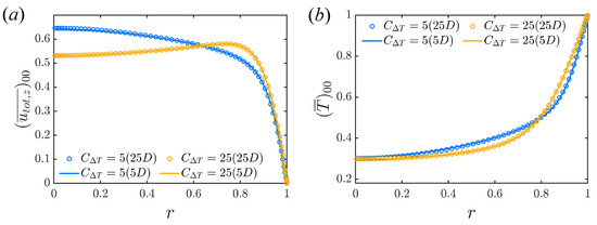
Figure 9. Comparison of mean (a) streamwise velocity and (b) temperature profile between short periodic pipe ($L=5D$) and long periodic pipe ($L=25D$). Two typical flow states are simulated, i.e., shear turbulence ($C_{\Delta T}=5$) and convective turbulence ($C_{\Delta T}=25$) at $Re=5300$. The fixed temperature difference boundary condition is used.

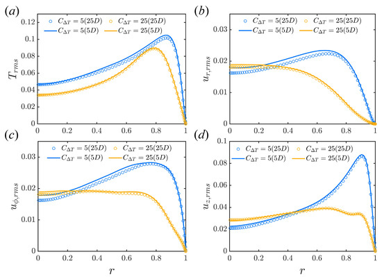
Figure 10. Comparison of (a) $T_{rms}$, (b) $u_{r,rms}$,(c) $u_{\varphi ,rms}$ and (d) $u_{z,rms}$ between short periodic pipe ($L=5D$) and long periodic pipe ($L=25D$). Two typical flow states are simulated, i.e., shear turbulence ($C_{\Delta T}=5$) and convective turbulence ($C_{\Delta T}=25$) at $Re=5300$. Fixed temperature difference.

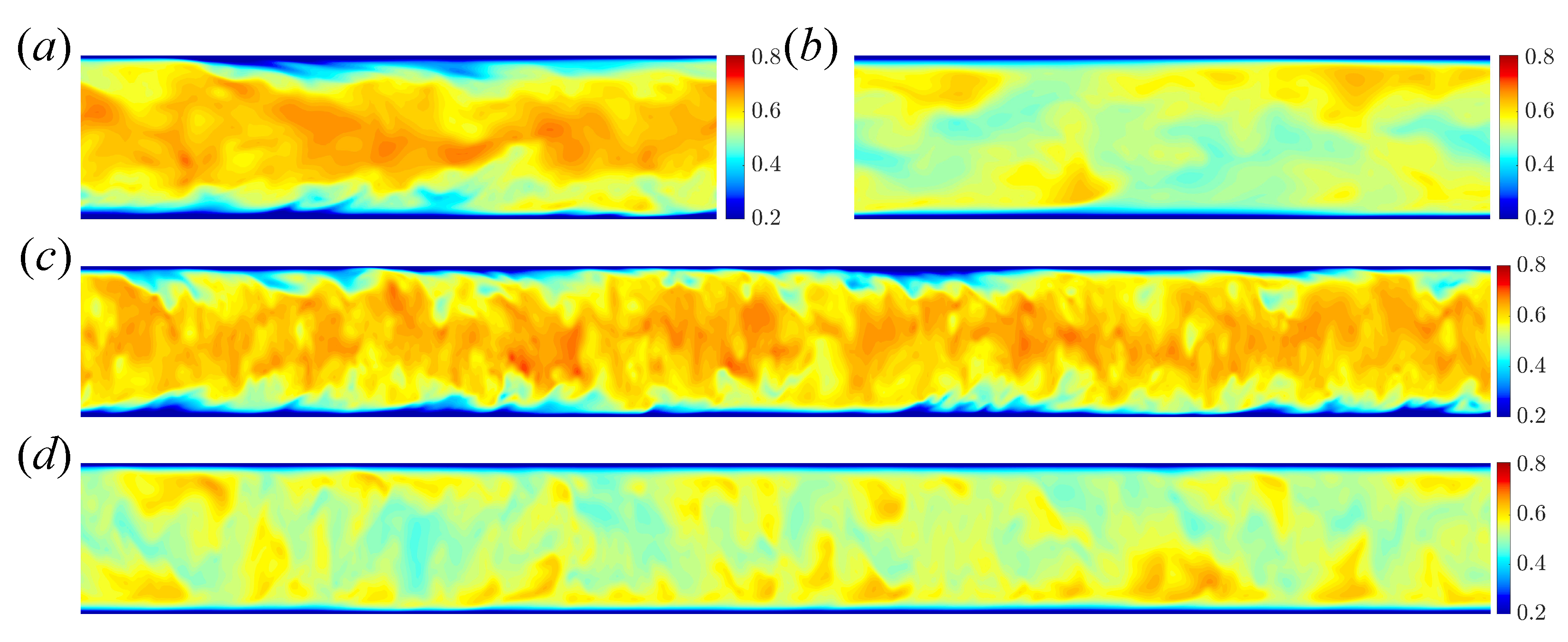
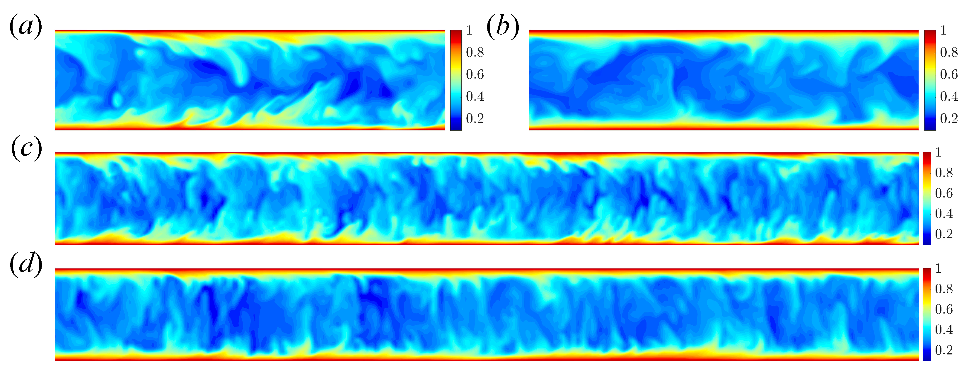
Contours of streamwise velocity and temperature in the $rz$ cross section for the two pipe lengths are shown in Figure 11 and Figure 12, respectively. The difference in velocity between the shear turbulence (Figure 11a,c) and convective turbulence (Figure 11b,d) is clear: shear turbulence has strong low-speed regions near the wall (associated with streaks). These are essentially absent in convective turbulence, and are replaced with localised regions of fast flow near the wall, while the core flow moves more slowly. No obvious difference in the contour plots is observed between short and long pipes, for both velocity and temperature fields.

Figure 11. Contours of streamwise velocity in $rz$ cross section for shear turbulence ($C_{\Delta T}=5$) in (a) $L=5D$, (c) $L=25D$, and convective turbulence ($C_{\Delta T}=25$) in (b) $L=5D$, (d) $L=25D$ at $Re=5300$. For the long pipe, the z-axis is scaled to show the whole pipe.

Figure 12. Contours of temperature in $rz$ cross-section for shear turbulence ($C_{\Delta T}=5$) in (a) $L=5D$, (c) $L=25D$, and convective turbulence ($C_{\Delta T}=25$) in (b) $L=5D$, (d) $L=25D$ at $Re=5300$. For the long pipe, the z-axis is scaled to show the whole pipe.

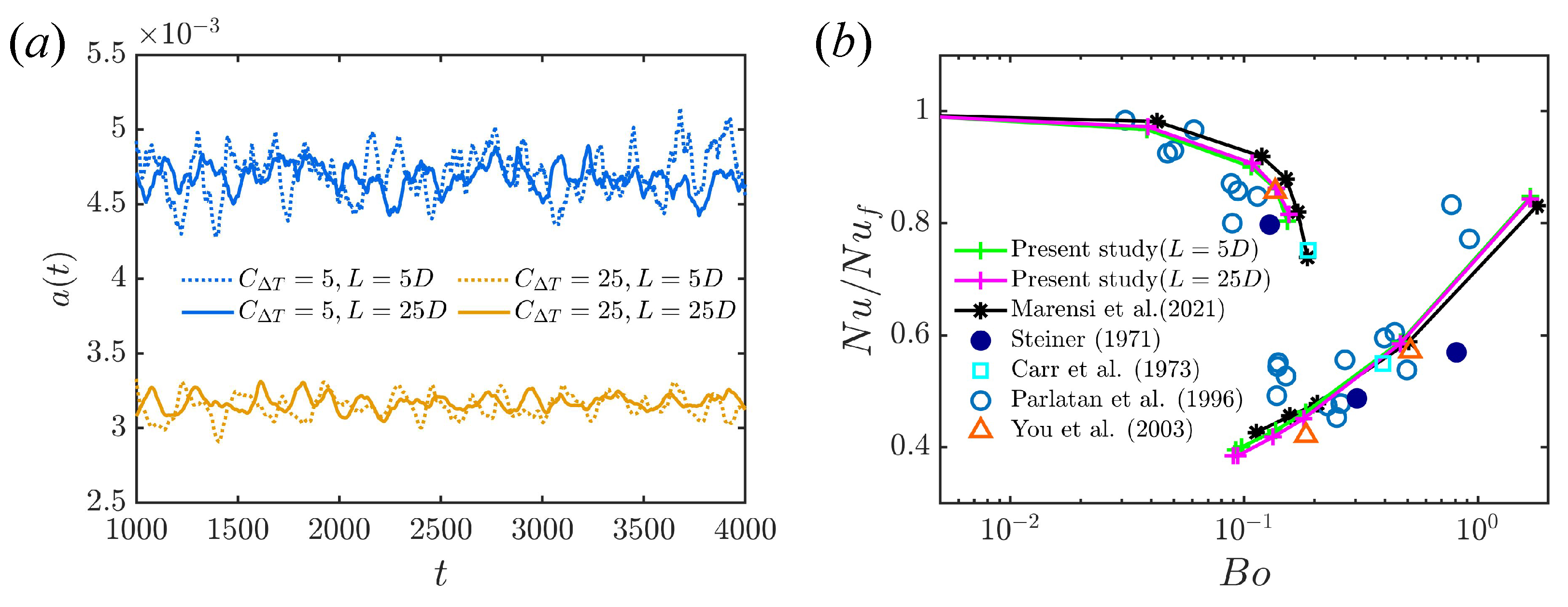
The time evolution of $a\left(t\right)$ for the two pipe lengths is shown in Figure 13a. The curves at matching $C_{\Delta T}$ are quite close, but smaller fluctuations in $a\left(t\right)$ are observed for the longer pipe. This is expected, as the larger domain gives more steady volume-averaged quantities used in the calculation of $a\left(t\right)$. Nusselt numbers for the short and long pipes at several $C_{\Delta T}$ are compared in Figure 13b. There is almost no difference in the Nusselt number over a wide range $C_{\Delta T}$ covering both shear turbulence and convective turbulence. Therefore, it is concluded that the simulation of a short periodic pipe ($L=5D$) is enough to predict the heat transfer and flow dynamics for fully turbulent flow. For C close to critical, however, data from either one state or the other are used in the calculation of $\mathit{Nu}$ so that intermittency is not fully accounted for. We consider this next.

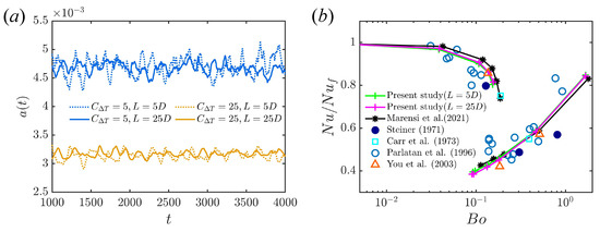
Figure 13. (a) Time evolution of $a\left(t\right)$ for short ($L=5D$) and longer pipe ($L=25D$). (b) Normalised Nusselt number for the short and longer pipe at $Re=5300$. $Bo$ defined as in Figure 3. Fixed temperature difference model. Data from [6,20,35,36,37].

In isothermal flow, localised turbulent patches are called puffs and slugs [39]. Puffs appear for $Re\approx 1800$ and are statistically steady in axial extent. From $Re\gtrsim 2250$, they start to expand and are called slugs. However, within the expanding turbulent region (that will eventually fill a periodic domain), laminar patches remain present for $Re$ up to approximately 2800 [40]. Thus, there is a large range over which the intermittent nature of turbulence cannot be captured in a short periodic domain of length $L=5D$. Puffs and slugs have frictional drag between the values extrapolated from the fully turbulent or laminar regimes, and are marked as a hatched area in the Moody diagram [41]. For a heated pipe, this will affect the estimations of $\mathit{Nu}$.

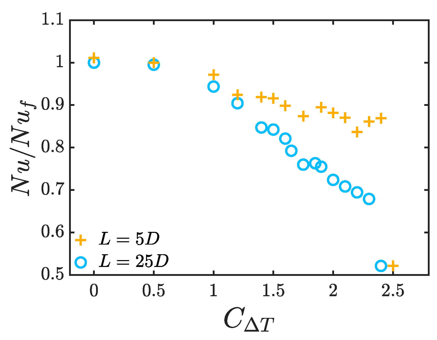
In vertical heated pipe flow, intermittent turbulence exists around the boundary between laminar and shear turbulence at higher Reynolds numbers, at the meeting of the green and blue regions in Figure 4. Examples of puff and slug at $Re=3000,C_{\Delta T}=1.9$ are shown in Figure 14. Nusselt numbers for the short and long pipes at $Re=3000$ are shown in Figure 15. At small $C_{\Delta T}$, there is almost no difference, as the turbulence fills the pipe. As $C_{\Delta T}$ increases, the difference in $\mathit{Nu}$ between the short and long pipe becomes substantial, due to the appearance of localised turbulence. Eventually, laminarisation occurs, marked by the final two points.

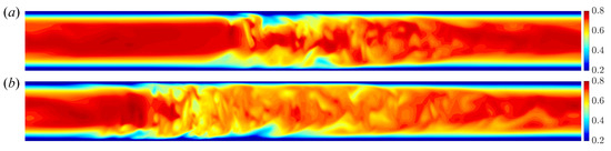
Figure 14. Contour of streamwise velocity in long pipe ($L=25D$ at $Re=3000,C_{\Delta T}=1.9$): $\left(\mathit{a}\right)$ puff and $\left(\mathit{b}\right)$ slug.

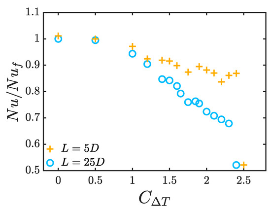
Figure 15. Comparison of Nusselt number for transitional $C_{\Delta T}$ for a short and long periodic domain ($L=5D,25D$) at $Re=3000$. Values for (intermittent) turbulence are shown, except for the final two laminar points.

3.3. The Lifetime of Localised Shear Turbulence

The mean lifetimes of turbulent puffs in isothermal flow, and its scaling with Reynolds number, have been closely investigated [28,42,43,44]. At each $Re$, the mean lifetime must be estimated from a series of simulations or experiments, and data are often truncated, due to the limited simulation time or the finite length of the pipe [28]. To examine whether the lifetime of puffs in heated pipes behave similarly, we calculate the survivor functions at $Re=3000$ for several $C_{\Delta T}$. To generate the initial conditions for the simulations, a localised disturbance is applied to the laminar Poiseuille flow at $Re=3000,C_{\Delta T}=1.9$ and the resulting puff is evolved for $t\approx$5000. Snapshots of the full velocity field are recorded every 20 time units, generating a large collection of initial conditions. Subsequently, simulations at larger $C_{\Delta T}$ are performed starting from these initial conditions and are monitored until the flow laminarises. The criterion for laminarisation is $E_{3d}<{10}^{-3}$, below which turbulent motions are decayed beyond recovery.

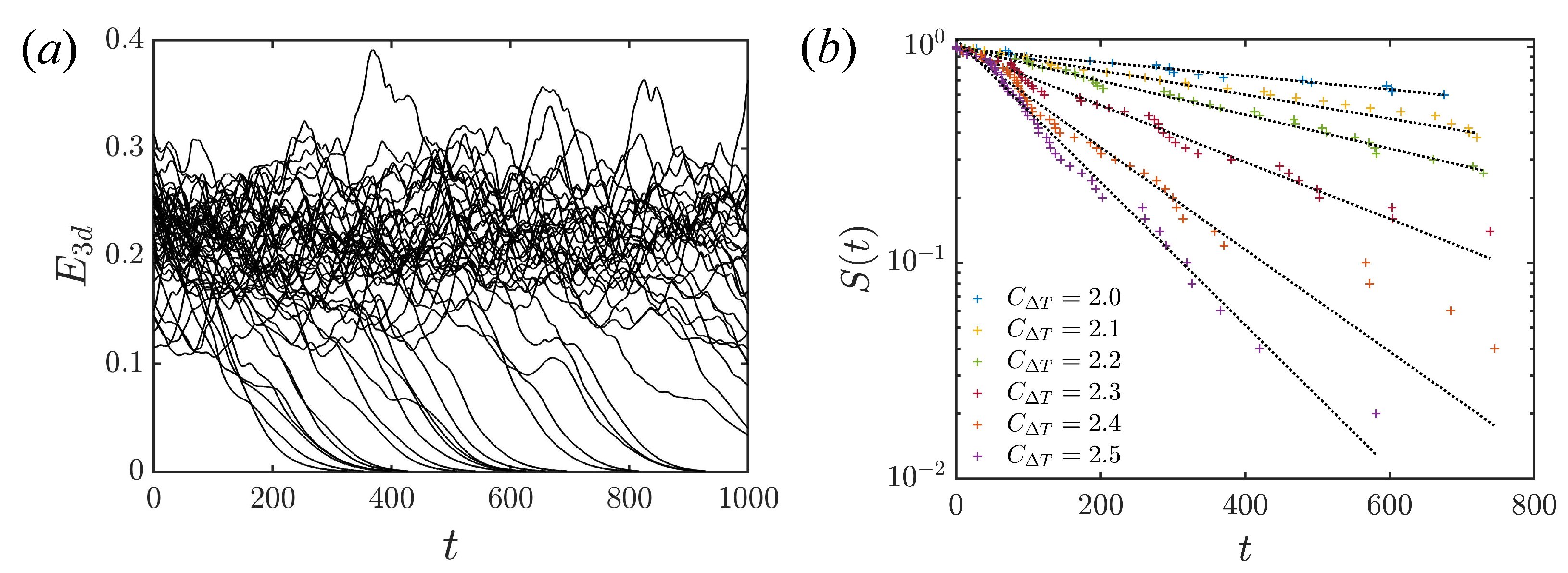
The time evolution of $E_{3d}$ of $n=50$ arbitrary initial turbulent fields at $C_{\Delta T}=2$ are shown in Figure 16a. Some cases decay to the laminar state, while others remain turbulent for the period of the simulation. The decay of turbulence leads to a large drop in the Nusselt number and an exponential decay of $E_{3d}$ so that laminarisations are clearly identifiable. For a finite set of samples, the survivor function is approximated by

$$S\left(t\right)={\displaystyle \frac{r}{n}},$$

(23)

where r is the number of puffs that survive up to time t. For example, all initial conditions survive before $t=10$, then $S\left(t\right)=1$ when $t<10$. In this way, we can calculate the lifetime of survivor probability from 1 to ${\displaystyle \frac{1}{50}}$. However, due to the finite time it takes for $E_{3d}$ to drop to ${10}^{-3}$, the data in Figure 16b are shifted to the left by the time of the earliest decay (≈250). As $C_{\Delta T}$ increases, the mean lifetime of puffs decreases. The distributions remain exponential in form for each $C_{\Delta T}$. This indicates that the puff decay induced by heating is also a memoryless process, corresponding to the escape from a strange saddle [28,42]. The enhancement of heating has a similar effect to that of the decrease in Reynolds number in isothermal flow.

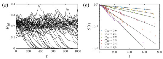
Figure 16. The time evolution of $\left(\mathit{a}\right)$$E_{3d}$ of 50 arbitrary initial turbulent fields at $C_{\Delta T}=2$. $\left(\mathit{b}\right)$ Survivor function for several values of the buoyancy parameter. $n=50$ samples for each case. $L=25D$.

4. Conclusions

In this work, we have presented a derivation of a model for vertically heated pipe flow that includes a time-dependent axial temperature gradient. This gradient adjusts in response to the flow pattern. A transition from shear turbulence to convective turbulence is well known to lead to a drop in heat transfer. For the fixed temperature model, reduced heat transferred into the fluid leads to a reduction in the temperature gradient. With the fixed heat flux boundary condition, however, as the energy withdrawn from the domain is proportional to the gradient, the gradient is forced to remain the same on average to match the energy entering the domain.

Laminar solutions are calculated numerically for several values of the buoyancy parameter, and are consistent with previous reports [6,20,31]. For turbulent flow, the time-averaged velocity and temperature profiles, and their RMS fluctuations, are calculated for both boundary conditions. The two turbulent regimes, i.e., shear turbulence and convective turbulence, are easily distinguished in the mean profiles and RMS flucutations. The dependence of flow state over the space of $Re$ and $\mathit{Nu}$ is calculated for both boundary conditions along with various statistics. Statistics show minor differences between the boundary conditions, but both show good consistency with the previous calculations and experiments. Of particular interest are the RMS temperature fluctuations, as they can be non-zero at the wall for the fixed-flux case. Also of interest is that convective turbulence can trigger bursts of shear-like turbulence when close to the critical C between the two states (For isothermal flow, shear-turbulence cannot return from the linearly stable laminar state).

Further simulations are carried out to examine the effect of the periodic length of the pipe on the turbulent statistics and heat transfer. The short pipe $L=5D$ and long pipe $L=25D$ show almost no difference in the mean velocity and mean temperature profiles. However, there are some minor mismatches in the RMS of velocity and temperature. The length of the pipe is found to have more effect on shear turbulent state, possibly due to spatial intermittency. The mismatch mainly appears in the centre of the pipe, while there is always a good agreement in the near-wall regime. Hence, the short pipe still captures accurate Nusselt numbers, provided that the flow is not too intermittent. In that case, simulations with a short pipe are likely to overestimate heat transfer, as shear turbulence fills the domain.

Finally, we have recorded the lifetime of the localised turbulence with heating, confirming it also follows a memoryless process corresponding to the escape from a strange saddle. Using the previous model of [6] close to criticality at larger $Re$, strong fronts and puffs have been found to disappear [45].

The code used for these calculations is available at openpipeflow.org (accessed on 15 March 2024).

References

- Zhang, S.; Xu, X.; Liu, C.; Dang, C. A review on application and heat transfer enhancement of supercritical CO2 in low-grade heat conversion. Appl. Energy 2020, 269, 114962. [Google Scholar] [CrossRef]
- McEligot, D.; Coon, C.; Perkins, H. Relaminarization in tubes. Int. J. Heat Mass Transf. 1970, 13, 431–433. [Google Scholar] [CrossRef]
- Ackerman, J. Pseudoboiling heat transfer to supercritical pressure water in smooth and ribbed tubes. J. Heat Transf. Trans. ASME 1970, 92, 490–498. [Google Scholar] [CrossRef]
- Bae, J.H.; Yoo, J.Y.; Choi, H. Direct numerical simulation of turbulent supercritical flows with heat transfer. Phys. Fluids 2005, 17, 105104. [Google Scholar] [CrossRef]
- Wibisono, A.F.; Addad, Y.; Lee, J.I. Numerical investigation on water deteriorated turbulent heat transfer regime in vertical upward heated flow in circular tube. Int. J. Heat Mass Transf. 2015, 83, 173–186. [Google Scholar] [CrossRef]
- Marensi, E.; He, S.; Willis, A.P. Suppression of turbulence and travelling waves in a vertical heated pipe. J. Fluid Mech. 2021, 919, A17. [Google Scholar] [CrossRef]
- Chu, S.; Willis, A.P.; Marensi, E. The minimal seed for transition to convective turbulence in heated pipe flow. J. Fluid Mech. 2024, 997, A46. [Google Scholar] [CrossRef]
- Hall, W.B.; Jackson, J. Laminarization of a turbulent pipe flow by buoyancy forces. In Proceedings of the Mechanical Engineering; ASME—American Society of Mechanical Engineers: New York, NY, USA, 1969; Volume 91, p. 66. [Google Scholar]
- He, S.; He, K.; Seddighi, M. Laminarisation of flow at low Reynolds number due to streamwise body force. J. Fluid Mech. 2016, 809, 31–71. [Google Scholar] [CrossRef]
- Hof, B.; De Lozar, A.; Avila, M.; Tu, X.; Schneider, T.M. Eliminating turbulence in spatially intermittent flows. Science 2010, 327, 1491–1494. [Google Scholar] [CrossRef] [PubMed]
- Kühnen, J.; Song, B.; Scarselli, D.; Budanur, N.B.; Riedl, M.; Willis, A.P.; Avila, M.; Hof, B. Destabilizing turbulence in pipe flow. Nat. Phys. 2018, 14, 386–390. [Google Scholar] [CrossRef]
- Scheele, G.F.; Hanratty, T.J. Effect of natural convection on stability of flow in a vertical pipe. J. Fluid Mech. 1962, 14, 244–256. [Google Scholar] [CrossRef]
- Chu, S.; Willis, A.P.; Marensi, E. Laminarising turbulent pipe flow by linear and nonlinear optimisation. arXiv 2024, arXiv:2410.19699. [Google Scholar]
- Hamilton, J.M.; Kim, J.; Waleffe, F. Regeneration mechanisms of near-wall turbulence structures. J. Fluid Mech. 1995, 287, 317–348. [Google Scholar] [CrossRef]
- Hiroaki, T.; Ayao, T.; Masaru, H.; Nuchi, N. Effects of buoyancy and of acceleration owing to thermal expansion on forced turbulent convection in vertical circular tubes—criteria of the effects, velocity and temperature profiles, and reverse transition from turbulent to laminar flow. Int. J. Heat Mass Transf. 1973, 16, 1267–1288. [Google Scholar] [CrossRef]
- Cotton, M.A. Theoretical Studies of Mixed Convection in Vertical Tubes. Ph.D. Thesis, University of Manchester, Manchester, UK, 1986. [Google Scholar]
- Launder, B.E.; Sharma, B.I. Application of the energy-dissipation model of turbulence to the calculation of flow near a spinning disc. Lett. Heat Mass Transf. 1974, 1, 131–137. [Google Scholar] [CrossRef]
- Behzadmehr, A.; Galanis, N.; Laneville, A. Low Reynolds number mixed convection in vertical tubes with uniform wall heat flux. Int. J. Heat Mass Transf. 2003, 46, 4823–4833. [Google Scholar] [CrossRef]
- Kasagi, N.; Nishimura, M. Direct numerical simulation of combined forced and natural turbulent convection in a vertical plane channel. Int. J. Heat Fluid Flow 1997, 18, 88–99. [Google Scholar] [CrossRef]
- You, J.; Yoo, J.Y.; Choi, H. Direct numerical simulation of heated vertical air flows in fully developed turbulent mixed convection. Int. J. Heat Mass Transf. 2003, 46, 1613–1627. [Google Scholar] [CrossRef]
- Kim, W.; He, S.; Jackson, J. Assessment by comparison with DNS data of turbulence models used in simulations of mixed convection. Int. J. Heat Mass Transf. 2008, 51, 1293–1312. [Google Scholar] [CrossRef]
- Chu, X.; Laurien, E.; McEligot, D.M. Direct numerical simulation of strongly heated air flow in a vertical pipe. Int. J. Heat Mass Transf. 2016, 101, 1163–1176. [Google Scholar] [CrossRef]
- Antoranz, A.; Gonzalo, A.; Flores, O.; Garcia-Villalba, M. Numerical simulation of heat transfer in a pipe with non-homogeneous thermal boundary conditions. Int. J. Heat Fluid Flow 2015, 55, 45–51. [Google Scholar] [CrossRef]
- Straub, S.; Forooghi, P.; Marocco, L.; Wetzel, T.; Vinuesa, R.; Schlatter, P.; Frohnapfel, B. The influence of thermal boundary conditions on turbulent forced convection pipe flow at two Prandtl numbers. Int. J. Heat Mass Transf. 2019, 144, 118601. [Google Scholar] [CrossRef]
- Cruz, R.V.; Flageul, C.; Lamballais, E.; Duffal, V.; Le Coupanec, E.; Benhamadouche, S. High-fidelity simulation of turbulent mixed convection in pipe flow. Int. J. Heat Fluid Flow 2024, 110, 109640. [Google Scholar] [CrossRef]
- Willis, A.P. The Openpipeflow Navier–Stokes solver. SoftwareX 2017, 6, 124–127. [Google Scholar] [CrossRef]
- Eggels, J.G.; Unger, F.; Weiss, M.; Westerweel, J.; Adrian, R.J.; Friedrich, R.; Nieuwstadt, F.T. Fully developed turbulent pipe flow: A comparison between direct numerical simulation and experiment. J. Fluid Mech. 1994, 268, 175–210. [Google Scholar] [CrossRef]
- Avila, M.; Willis, A.P.; Hof, B. On the transient nature of localized pipe flow turbulence. J. Fluid Mech. 2010, 646, 127–136. [Google Scholar] [CrossRef]
- Gray, D.D.; Giorgini, A. The validity of the Boussinesq approximation for liquids and gases. Int. J. Heat Mass Transf. 1976, 19, 545–551. [Google Scholar] [CrossRef]
- Turner, J.S.; Turner, J.S. Buoyancy Effects in Fluids; Cambridge University Press: Cambridge, UK, 1979. [Google Scholar]
- Su, Y.C.; Chung, J.N. Linear stability analysis of mixed-convection flow in a vertical pipe. J. Fluid Mech. 2000, 422, 141–166. [Google Scholar] [CrossRef]
- Piller, M. Direct numerical simulation of turbulent forced convection in a pipe. Int. J. Numer. Methods Fluids 2005, 49, 583–602. [Google Scholar] [CrossRef]
- Baranovskii, E.S.; Domnich, A.A.; Artemov, M.A. Mathematical Analysis of the Poiseuille Flow of a Fluid with Temperature-Dependent Properties. Mathematics 2024, 12, 3337. [Google Scholar] [CrossRef]
- Yoo, J.Y. The turbulent flows of supercritical fluids with heat transfer. Annu. Rev. Fluid Mech. 2013, 45, 495–525. [Google Scholar] [CrossRef]
- Steiner, A. On the reverse transition of a turbulent flow under the action of buoyancy forces. J. Fluid Mech. 1971, 47, 503–512. [Google Scholar] [CrossRef]
- Carr, A.; Connor, M.; Buhr, H. Velocity, Temperature, and Turbulence Measurements in Air for Pipe Flow with Combined Free and Forced Convection. J. Heat Transf. 1973, 95, 445–452. [Google Scholar] [CrossRef]
- Parlatan, Y.; Todreas, N.; Driscoll, M. Buoyancy and property variation effects in turbulent mixed convection of water in vertical tubes. J. Heat Transf. 1996, 118, 381–387. [Google Scholar] [CrossRef]
- Zhao, P.; Zhu, J.; Ge, Z.; Liu, J.; Li, Y. Direct numerical simulation of turbulent mixed convection of LBE in heated upward pipe flows. Int. J. Heat Mass Transf. 2018, 126, 1275–1288. [Google Scholar] [CrossRef]
- Avila, M.; Barkley, D.; Hof, B. Transition to turbulence in pipe flow. Annu. Rev. Fluid Mech. 2023, 55, 575–602. [Google Scholar] [CrossRef]
- Marensi, E.; Hof, B. The onset of fully turbulent pipe flow. In Proceedings of the APS Division of Fluid Dynamics Meeting Abstracts, Phoenix, AZ, USA, 21–23 November 2021; p. P31012M. [Google Scholar]
- Moody, L.F. Friction Factors for Pipe Flow. J. Fluids Eng. 1944, 66, 671–678. [Google Scholar] [CrossRef]
- Willis, A.; Kerswell, R. Critical behavior in the relaminarization of localized turbulence in pipe flow. Phys. Rev. Lett. 2007, 98, 014501. [Google Scholar] [CrossRef] [PubMed]
- Willis, A.P.; Kerswell, R.R. Turbulent dynamics of pipe flow captured in a reduced model: Puff relaminarization and localized ‘edge’states. J. Fluid Mech. 2009, 619, 213–233. [Google Scholar] [CrossRef]
- Hof, B.; de Lozar, A.; Kuik, D.; Westerweel, J. Repeller or attractor? Selecting the dynamical model for the onset of turbulence in pipe flow. Phys. Rev. Lett. 2008, 101, 214501. [Google Scholar] [CrossRef] [PubMed]
- Zhuang, Y.; Yang, B.; Mukund, V.; Marensi, E.; Hof, B. Discontinuous transition to shear flow turbulence. arXiv 2023, arXiv:2311.11474. [Google Scholar]
Disclaimer/Publisher’s Note: The statements, opinions and data contained in all publications are solely those of the individual author(s) and contributor(s) and not of MDPI and/or the editor(s). MDPI and/or the editor(s) disclaim responsibility for any injury to people or property resulting from any ideas, methods, instructions or products referred to in the content. |
© 2025 by the authors. Licensee MDPI, Basel, Switzerland. This article is an open access article distributed under the terms and conditions of the Creative Commons Attribution (CC BY) license (https://creativecommons.org/licenses/by/4.0/).