Backstepping Sliding Mode Control of Quadrotor UAV Trajectory

Abstract

Unmanned Aerial Vehicles (UAVs), commonly known as drones, have become widely used in many fields, ranging from agriculture to military operations, due to recent advances in technology and decreases in costs. Quadrotors are particularly important UAVs, but their complex, coupled dynamics and sensitivity to outside disturbances make them challenging to control. This paper introduces a new control method for quadrotors called Backstepping Sliding Mode Control (BSMC), which combines the strengths of two established techniques: Backstepping Control (BC) and Sliding Mode Control (SMC). Its primary goal is to improve trajectory tracking while also reducing chattering, a common problem with SMC that causes rapid, high-frequency oscillations. The BSMC method achieves this by integrating the SMC switching gain directly into the BC through a process of differential iteration. Herein, a Lyapunov stability analysis confirms the system’s asymptotic stability; a genetic algorithm is used to optimize controller parameters; and the proposed control strategy is evaluated under diverse payload conditions and dynamic wind disturbances. The simulation results demonstrated its capability to handle payload variations ranging from 0.5 kg to 18 kg in normal environments, and up to 12 kg during gusty wind scenarios. Furthermore, the BSMC effectively minimized chattering and achieved a superior performance in tracking accuracy and robustness compared to the traditional SMC and BC.

1. Introduction

Unmanned Aerial Vehicles (UAVs), commonly known as drones, have gained increasing popularity due to their versatility and wide range of applications in both civilian and military fields. Their capabilities extend to surveillance [1,2], search and rescue missions [3,4,5,6], infrastructure inspections [7,8], and tactical operations [9], among many others. Among the various UAV configurations, the quadrotor stands out for its vertical take-off and landing (VTOL) capabilities, hovering stability, mechanical simplicity, and agility. This type of rotorcraft features four independent rotors for propulsion and control, making it well-suited for complex missions in constrained or hazardous environments.

The growing interest in quadrotors has been driven by their maneuverability and suitability for tasks requiring precise control. However, despite their apparent simplicity, quadrotors are characterized by complex dynamics, including strong nonlinearities, multiple-input multiple-output (MIMO) coupling, and under actuation. These challenges are compounded by the presence of external disturbances, model uncertainties, and actuator limitations [10,11,12,13]; hence, effective control of quadrotor UAVs remains a central challenge in aerial robotics research.

To address these issues, researchers have explored a wide range of control strategies. Traditional methods such as Proportional–Integral–Derivative (PID) controllers and Linear Quadratic Regulators (LQRs) have been extensively applied by linearizing the system around operating modes like hovering or steady flight [14,15,16,17,18]. While these techniques offer simplicity and intuitive design, they often suffer from performance degradation under significant deviations from these linearized points due to the inherently nonlinear nature of the system [19,20,21,22].

More robust nonlinear control techniques, such as Sliding Mode Control (SMC), have demonstrated a superior performance in terms of disturbance rejection and robustness to parameter uncertainties [23,24,25,26]. However, the key drawback of SMC is the chattering phenomenon, a high-frequency switching behavior that can excite unmodeled dynamics, increase wear on mechanical components, and generate thermal stress in actuators. Moreover, many existing studies neglect the effect of actuator dynamics, which is critical for achieving realistic and implementable control in practical systems.

Recent advances in quadrotor control include adaptive and terminal SMC [27], and intelligent control strategies such as neural-network-based backstepping and model predictive control [28,29]. While these approaches achieve excellent tracking performance, they often require online parameter adaptation, computationally expensive optimization, or training of learning-based components, which may limit their applicability for resource-constrained UAVs. In contrast, the proposed BSMC retains the low complexity of classical methods while improving tracking performance and robustness, making it well-suited for real-time applications.

In [30], the authors proposed a robust adaptive fault-tolerant control scheme for quadrotor UAVs by combining sliding mode control with adaptive laws to handle unknown disturbances and abrupt actuator faults. Their method demonstrated strong performance under actuator faults and external disturbances but requires an additional adaptive law for parameter updating, which increases implementation complexity.

In [31], the authors developed a fractional-order sliding mode observer for actuator fault estimation in quadrotor UAVs. This work highlights the trend of using fractional-order sliding mode approaches to improve estimation accuracy and robustness. However, fractional-order implementation may require higher computational resources and careful tuning of fractional parameters.

These studies illustrate the growing interest in robust and fault-tolerant control schemes for UAVs. Unlike these approaches, the proposed BSMC focuses on enhancing classical controllers (SMC and BSC) by combining their strengths and tuning parameters via Genetic Algorithm (GA) optimization, resulting in a simpler design that achieves high accuracy and robustness without additional adaptive or fractional-order structures.

In recent years, hybrid strategies that combine the strengths of multiple control techniques have been proposed to overcome these limitations, among which the Backstepping Sliding Mode Control (BSMC) method stands out as a promising solution. By integrating Backstepping design with SMC, BSMC achieves a robust performance while reducing chattering effects. Furthermore, the Backstepping framework allows dynamic estimation of the switching gain in SMC, which enables it to adaptively compensate for disturbances and uncertainties [32,33,34,35,36,37,38].

This study introduces a reliable and practical control method designed to improve the real-world performance of a quadrotor. The method is particularly effective when the quadrotor operates in unpredictable and changing conditions, like those with varying payloads and sudden wind gusts. To ensure stability, the control law is based on Lyapunov theory, and the control parameters are tuned using a genetic algorithm (GA), which optimizes their performance. The effectiveness of this approach is confirmed through several simulations that tested the method’s ability to handle different payloads and wind disturbances.

The main goal of this work is to enhance the tracking performance of classical controllers, specifically Sliding Mode Control (SMC) and Backstepping Control (BSC), by combining them into a unified Backstepping Sliding Mode Controller (BSMC). Therefore, the evaluation focuses on comparing BSMC against its constituent controllers to clearly demonstrate the performance improvement. The main contributions of this study are as follows:

• The development of a dynamic model for a Quadrotor UAV (QUAV).
• The design of a BSMC strategy that reduces chattering while ensuring robust performance and stability.
• The optimization of the controller parameters using a GA.

This paper is organized as follows: Section 1 provides an introduction to the research; Section 2 outlines the modeling framework in detail; Section 3 provides an explanation of the BSMC’s design and the tuning of the controller parameters by GA; Section 4 presents the simulation results and discussion; and, finally, Section 5 concludes the research.

2. Modeling Approach of a Quadrotor UAV

2.1. Kinematic Model

2.1.1. Reference Frame Alignment

Since a quadrotor can maneuver in six degrees of freedom, six variables are needed to fully define its spatial position and orientation. To accurately analyze its motion, two reference frames are essential: the body frame, which moves with the quadrotor, and the inertial frame, which remains fixed in space. The quadrotor has various sensors, such as a gyroscope and accelerometer, which provide measurements relative to the body frame to determine the linear and angular velocity; additionally, a magnetometer or Global Positioning System (GPS), for example, can provide measurements relative to the inertial frame to determine the linear and angular position [39]. Figure 1 [40] is the reference frames for a quadrotor.

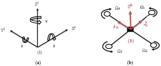
Figure 1. Reference frames: (a) inertial frame; (b) body-fixed frame [40].

The absolute linear position of the quadrotor’s center of mass in the inertial frame is expressed as

$${\xi }^I={\left[\begin{array}{ccc}X& Y& Z\end{array}\right]}^T$$

(1)

The attitude or the angular position in the inertial frame is defined with the ‘roll–pitch–yaw’ Euler angles:

$${\eta }^I={\left[\begin{array}{ccc}\varphi & \theta & \psi \end{array}\right]}^T,$$

(2)

The linear velocity $V^B$ and angular velocity $v^B$ are defined in the body-fixed frame as

$$V^B={\left[\begin{array}{ccc}{v}_x& v_y& v_z\end{array}\right]}^T,$$

(3)

$$v^B={\left[\begin{array}{ccc}P& Q& R\end{array}\right]}^T$$

(4)

The net thrust acting on the quadrotor $T_{net}^B$ and net rotational moment ${\tau }_{net}^B$ are defined in the body-fixed frame as

$$T_{net}^B={\left[\begin{array}{ccc}0& 0& T\end{array}\right]}^T,$$

(5)

$${\tau }_{net}^B={\left[\begin{array}{ccc}{\tau }_{\varphi }& {\tau }_{\theta }& {\tau }_{\psi }\end{array}\right]}^T$$

(6)

2.1.2. Rotation and Transformation Matrix

A rotation matrix is used to convert the quadrotor’s net thrust and rotational moment from its body frame to the inertial frame. This transformation is achieved through a sequence of rotations about the principal axes—first, around the $Z$-axis; then, the $Y$ axis; and finally, the $X$-axis. Rotation matrices about the $Z$-axis with angle $\psi$, rotation about the $Y$-axis with angle $\theta$, and rotation about the $X$-axis with angle $\varphi$ are given by

$$R_{z,\psi }=\left[\begin{array}{ccc}\mathrm{c}\mathrm{o}\mathrm{s}\psi & -\mathrm{s}\mathrm{i}\mathrm{n}\psi & 0\\ \mathrm{s}\mathrm{i}\mathrm{n}\psi & \mathrm{c}\mathrm{o}\mathrm{s}\psi & 0\\ 0& 0& 1\end{array}\right], R_{y,\theta }=\left[\begin{array}{ccc}\mathrm{c}\mathrm{o}\mathrm{s}\theta & 0& \mathrm{s}\mathrm{i}\mathrm{n}\theta \\ 0& 1& 0\\ -\mathrm{s}\mathrm{i}\mathrm{n}\theta & 0& \mathrm{c}\mathrm{o}\mathrm{s}\theta \end{array}\right] \mathrm{a}\mathrm{n}\mathrm{d} R_{x,\varphi }=\left[\begin{array}{ccc}1& 0& 0\\ 0& \mathrm{c}\mathrm{o}\mathrm{s}\varphi & -\mathrm{s}\mathrm{i}\mathrm{n}\varphi \\ 0& \mathrm{s}\mathrm{i}\mathrm{n}\varphi & \mathrm{c}\mathrm{o}\mathrm{s}\varphi \end{array}\right]$$

(7)

Combining these matrices in different orders can represent any arbitrary 3D rotation, given by

$$R_B^E=R_{z,\psi }\times R_{y,\theta }\times R_{x,\varphi }=\left[\begin{array}{ccc}{C}_{\psi }{C}_{\theta }& C_{\psi }{S}_{\theta }{S}_{\varphi }-S_{\psi }{C}_{\varphi }& C_{\psi }{S}_{\theta }{C}_{\varphi }+S_{\psi }{S}_{\varphi }\\ S_{\psi }{C}_{\theta }& S_{\psi }{S}_{\theta }{S}_{\varphi }+C_{\psi }{C}_{\varphi }& S_{\psi }{S}_{\theta }{C}_{\varphi }-C_{\psi }{S}_{\varphi }\\ -S_{\theta }& C_{\theta }{S}_{\varphi }& C_{\theta }{C}_{\varphi }\end{array}\right],$$

(8)

where $C_k=\mathrm{c}\mathrm{o}\mathrm{s}\left(k\right)$ and $S_k=\mathrm{s}\mathrm{i}\mathrm{n}\left(k\right)$. The rotation matrix $R_B^E$ is orthogonal and used to convert the body reference frame to the inertial reference frame. ${\left(R_B^E\right)}^{-1}={\left(R_B^E\right)}^T$ for $-\pi /2<\varphi$, $\theta <\pi /2$, and $-\pi <\psi <\pi$, which is the rotation matrix from the inertial frame to the body frame.

Also, transformation matrices including $T_M$, to convert angular velocities from the inertial frame to the body frame, and $T_M^{-1}$, to convert angular velocities from the body frame to the inertial frame, are needed. By using Equation (7), the transformation matrix T_M is calculated as follows [41]:

$$T_M\left[\begin{array}{c}\dot{\varphi }\\ \dot{\theta }\\ \dot{\psi }\end{array}\right]=R_{x,\varphi }{R}_{y,\theta }\left[\begin{array}{c}0\\ 0\\ \dot{\psi }\end{array}\right]+R_{x,\varphi }\left[\begin{array}{c}0\\ \dot{\theta }\\ 0\end{array}\right]+\left[\begin{array}{c}\dot{\varphi }\\ 0\\ 0\end{array}\right]=\left[\begin{array}{ccc}1& 0& -\mathit{sin}\theta \\ 0& \mathit{cos}\varphi & \mathit{cos}\theta \mathit{sin}\varphi \\ 0& -\mathit{sin}\varphi & \mathit{cos}\theta \mathit{cos}\varphi \end{array}\right]\left[\begin{array}{c}\dot{\varphi }\\ \dot{\theta }\\ \dot{\psi }\end{array}\right]$$

(9)

Its inverse $T_M^{-1}$ is given as follows:

$$T_M^{-1}=\left[\begin{array}{ccc}1& \mathit{sin}\varphi \mathit{tan}\theta & \mathit{cos}\varphi \mathit{tan}\theta \\ 0& \mathit{cos}\varphi & -\mathit{sin}\varphi \\ 0& \mathit{sin}\varphi /\mathit{cos}\theta & \mathit{cos}\varphi /\mathit{cos}\theta \end{array}\right]$$

(10)

By using Equations (9) and (10), it is possible to convert the angular velocities from the inertial frame to the body frame in a similar manner to converting the body frame to the inertial frame, as follows:

$$v^B=T_M{\dot{\eta }}^I, \left[\begin{array}{c}P\\ Q\\ R\end{array}\right]=T_M\left[\begin{array}{c}\dot{\varphi }\\ \dot{\theta }\\ \dot{\psi }\end{array}\right],$$

(11)

$${\dot{\eta }}^I=T_M^{-1}{v}^B, \left[\begin{array}{c}\dot{\varphi }\\ \dot{\theta }\\ \dot{\psi }\end{array}\right]=T_M^{-1}\left[\begin{array}{c}P\\ Q\\ R\end{array}\right]$$

(12)

2.2. Rigid Body Dynamics

The movement of the quadrotor consists of two components: rotational motion and translational motion. The translational motion relies on the alignment of the quadrotor, which is determined by its rotational movement; the rotational subsystem of the quadrotor is fully controllable. In the following sections, the equations describing the quadrotor’s rotational and translational motion are derived.

To model the behavior of the quadrotor system, the following assumptions are made [20]:

• The structure is assumed to be completely symmetrical and rigid.
• The center of mass of the quadrotor aligns with the origin of the body-fixed reference frame.
• Complex phenomena that are difficult to accurately simulate, such as ground effect, blade flapping, and other minor aerodynamic or inertial influences, are disregarded.

2.2.1. Rotational Equation of Motion

In the body frame, the rotational equation of the quadrotor motion is defined as [40]

$$I{\dot{v}}^B+v^B\times \left(I{v}^B\right)+{\tau }_{gyro}={\tau }_{net}^B,$$

(13)

where $I{\dot{v}}^B$ is an angular acceleration of the inertia, $v^B\times \left(I{v}^B\right)$ is a centripetal force, τ_gyro is a gyroscopic moment due to rotor inertia, and ${\tau }_{net}^B$ is net moments acting on the quadrotor due to the propeller’s movement. Inertia matrix, also known as the inertia tensor or moment of inertia matrix, is a mathematical representation of an object’s resistance to changes in rotational motion. Due to the assumption of a symmetric quadcopter frame, the inertia matrix is approximated by the moments of inertia around its principal axes.

$$I=diag(I_{xx},I_{yy},I_{zz}),$$

(14)

where $I_{xx}$, $I_{yy}$, and $I_{zz}$ are the moments of inertia about the principal axis in the body frame.

The gyroscopic moments arise from the rotation of the propellers and their interaction with the surrounding air. When the propellers rotate, they generate a torque that opposes any change in the quadrotor’s orientation; this torque is known as the gyroscopic moment. According to [40], gyroscopic torque is given as follows:

$${\tau }_{gyro}=J_r{v}^B\times \left[\begin{array}{c}0\\ 0\\ 1\end{array}\right]{\Omega }_r=J_r\left[\begin{array}{c}P\\ Q\\ R\end{array}\right]\times \left[\begin{array}{c}0\\ 0\\ 1\end{array}\right]({\Omega }_1-{\Omega }_2+{\Omega }_3-{\Omega }_4),$$

(15)

where $J_r$ and ${\Omega }_r$ are the rotor inertia and rotor relative speed, respectively. Each propeller rotates at an angular velocity ${\Omega }_i$, generating an upward force $f_i$ and a reactive torque ${\tau }_M$ that acts in the opposite direction of rotation. As illustrated in Figure 2, the propellers ${\Omega }_1$ and ${\Omega }_3$ rotate counterclockwise, while the remaining two rotate clockwise.

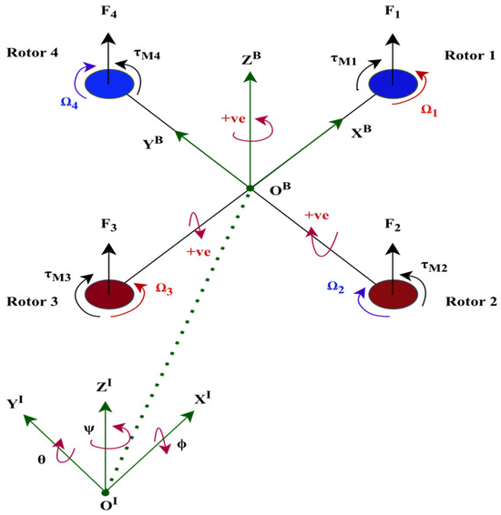
Figure 2. Schematic diagram of a quadrotor’s movement. The colors are used to identify between front and rear part of the quadrotors motor i.e., Blue (Front) and Brown (Rear) and the others are based on the direction of the rotation of the motors (Clockwise and Counterclockwise).

The thrust generated by the rotor $i$ is proportional to the square of the angular speed of the rotor and thrust constant $K_T$ [42]:

$$f_i=K_T{\Omega }_i^2$$

(16)

The torque developed around the rotor axis is given as the product of the square of the angular velocity and the drag coefficient $K_D$ [37]:

$${\tau }_{Mi}=K_D{\Omega }_i^2$$

(17)

The combined forces of the rotors create thrust $T$ in the direction of the body z-axis. Torque ${\tau }_{net}^B$ consists of the torques ${\tau }_{\varphi }$, ${\tau }_{\theta }$, and ${\tau }_{\psi }$ in the direction of the corresponding body frame angles.

$$T=K_T({\Omega }_1^2+{\Omega }_2^2+{\Omega }_3^2+{\Omega }_4^2),$$

(18)

$${\tau }_{net}^B=\left[\begin{array}{c}{\tau }_{\varphi }\\ {\tau }_{\theta }\\ {\tau }_{\psi }\end{array}\right]=\left[\begin{array}{c}l(-f_2+f_4)\\ l(-f_1+f_3)\\ {\sum }_{i=1}^4{\tau }_{Mi}\end{array}\right]=\left[\begin{array}{c}l{K}_T(-{\Omega }_2^2+{\Omega }_4^2)\\ l{K}_T(-{\Omega }_1^2+{\Omega }_3^2)\\ K_D({\Omega }_1^2-{\Omega }_2^2+{\Omega }_3^2-{\Omega }_4^2)\end{array}\right],$$

(19)

The distance between the center of mass of the quadrotor and the rotor is represented by $l$; thus, by combining Equations (14), (15), and (19), Equation (13) can be written as follows:

$$\begin{gathered} I{\dot{v}}^B+v^B\times \left(I{v}^B\right)+{\tau }_{gyro}={\tau }_{net}^B \\ \left[\begin{array}{ccc}{I}_{xx}& 0& 0\\ 0& I_{yy}& 0\\ 0& 0& I_{zz}\end{array}\right]\left[\begin{array}{c}\dot{P}\\ \dot{Q}\\ \dot{R}\end{array}\right]=-\left[\begin{array}{c}P\\ Q\\ R\end{array}\right]\times \left[\begin{array}{c}{I}_{xx}P\\ I_{yy}Q\\ I_{zz}R\end{array}\right]-J_r\left[\begin{array}{c}P\\ Q\\ R\end{array}\right]\times \left[\begin{array}{c}0\\ 0\\ 1\end{array}\right]{\Omega }_r+\left[\begin{array}{c}{\tau }_{\varphi }\\ {\tau }_{\theta }\\ {\tau }_{\psi }\end{array}\right], \end{gathered}$$

(20)

By rearranging Equation (20), the rotational equation of quadrotor motion in the body frame is derived as follows:

$$\left[\begin{array}{c}\dot{P}\\ \dot{Q}\\ \dot{R}\end{array}\right]=\left[\begin{array}{c}{\displaystyle \frac{(I_{yy}-I_{zz})QR}{I_{xx}}}-{\displaystyle \frac{Q{J}_r{\Omega }_r}{I_{xx}}}+{\displaystyle \frac{{\tau }_{\varphi }}{I_{xx}}}\\ {\displaystyle \frac{(I_{zz}-I_{xx})PR}{I_{yy}}}+{\displaystyle \frac{P{J}_r{\Omega }_r}{I_{yy}}}+{\displaystyle \frac{{\tau }_{\theta }}{I_{yy}}}\\ {\displaystyle \frac{(I_{xx}-I_{yy})PQ}{I_{zz}}}+{\displaystyle \frac{{\tau }_{\psi }}{I_{zz}}}\end{array}\right],$$

(21)

Using the transformation matrix $T_M^{-1}$, it is possible to convert the body frame to inertial reference frame as follows:

$$\left[\begin{array}{c}\dot{\varphi }\\ \dot{\theta }\\ \dot{\psi }\end{array}\right]=T_M^{-1}\left[\begin{array}{c}P\\ Q\\ R\end{array}\right],$$

(22)

2.2.2. Translational Equation of Motion

The quadrotor is assumed to be a rigid body and thus, Newton–Euler equations can be used to describe its translational dynamics [40] in the inertial frame. The equation of motion for translational motion is determined as follows [40]:

$$\begin{gathered} m\ddot{\xi }=\left[\begin{array}{c}0\\ 0\\ -mg\end{array}\right]+R_B^E{T}_{net}^B \\ m\left[\begin{array}{c}\ddot{X}\\ \ddot{Y}\\ \ddot{Z}\end{array}\right]=\left[\begin{array}{c}0\\ 0\\ -mg\end{array}\right]+\left[\begin{array}{ccc}{C}_{\psi }{C}_{\theta }& C_{\psi }{S}_{\theta }{S}_{\varphi }-S_{\psi }{C}_{\varphi }& C_{\psi }{S}_{\theta }{C}_{\varphi }+S_{\psi }{S}_{\varphi }\\ S_{\psi }{C}_{\theta }& S_{\psi }{S}_{\theta }{S}_{\varphi }+C_{\psi }{C}_{\varphi }& S_{\psi }{S}_{\theta }{C}_{\varphi }-C_{\psi }{S}_{\varphi }\\ -S_{\theta }& C_{\theta }{S}_{\varphi }& C_{\theta }{C}_{\varphi }\end{array}\right]\left[\begin{array}{c}0\\ 0\\ T\end{array}\right] \end{gathered}$$

(23)

Simplifying Equation (23) gives the final acceleration as

$$\left[\begin{array}{c}\ddot{X}\\ \ddot{Y}\\ \ddot{Z}\end{array}\right]=\left[\begin{array}{c}{\displaystyle \frac{T}{m}}(C_{\psi }{S}_{\theta }{C}_{\varphi }+S_{\psi }{S}_{\varphi })\\ {\displaystyle \frac{T}{m}}(S_{\psi }{S}_{\theta }{C}_{\varphi }-C_{\psi }{S}_{\varphi })\\ {\displaystyle \frac{T}{m}}\left(C_{\theta }{C}_{\varphi }\right)-g\end{array}\right],$$

(24)

2.3. State Space Representation of the Model

Finally, defining state variables as $x_1=X$, $x_2=\dot{X}$, $x_3=Y$, $x_4=\dot{Y}$, $x_5=Z$, $x_6=\dot{Z},$ $x_7=P$, $x_8=Q$, $x_9=R$, $x_{10}=\varphi$, $x_{11}=\theta$, and $x_{12}=\psi$ gives the state space representation of the overall quadrotor system as

$$\begin{gathered} {\dot{x}}_1=x_2 \\ {\dot{x}}_2={\displaystyle \frac{T}{m}}{U}_x+D_x \\ {\dot{x}}_3=x_4 \\ {\dot{x}}_4={\displaystyle \frac{T}{m}}{U}_y+D_y \\ {\dot{x}}_5=x_6 \\ {\dot{x}}_6=-g+{\displaystyle \frac{T}{m}}{U}_z+D_z \\ {\dot{x}}_7={\displaystyle \frac{I_{yy}-I_{zz}}{I_{xx}}}{x}_8{x}_9-{\displaystyle \frac{J_r}{I_{xx}}}{x}_8{\Omega }_r+{\displaystyle \frac{1}{I_{xx}}}{\tau }_{\varphi }+D_{\varphi } \\ {\dot{x}}_8={\displaystyle \frac{I_{zz}-I_{xx}}{I_{yy}}}{x}_7{x}_9+{\displaystyle \frac{J_r}{I_{yy}}}{x}_7{\Omega }_r+{\displaystyle \frac{1}{I_{yy}}}{\tau }_{\theta }+D_{\theta } \\ {\dot{x}}_9={\displaystyle \frac{I_{xx}-I_{yy}}{I_{zz}}}{x}_7{x}_8+{\displaystyle \frac{1}{I_{zz}}}{\tau }_{\psi }+D_{\psi } \\ {\dot{x}}_{10}=x_7+x_8\mathit{sin}(x_{10}\left)\mathit{tan}(x_{11}\right)+x_9\mathit{cos}(x_{10}\left)\mathit{tan}(x_{11}\right) \\ {\dot{x}}_{11}=x_8\mathit{cos}(x_{10})-x_9\mathit{sin}(x_{10}) \\ {\dot{x}}_{12}=x_8\mathit{sin}(x_{10})/\mathit{cos}(x_{11})+x_9\mathit{cos}(x_{10})/\mathit{cos}(x_{11}) \end{gathered}$$

(25)

where $D_x$, $D_y$, $D_z$, $D_{\varphi }$, $D_{\theta }$, and $D_{\psi }$ denote lumped disturbances and model uncertainties. These terms collectively capture unmodeled aerodynamic effects (e.g., ground effect, blade flapping, drag), actuator asymmetries, and parameter variations. Including these terms allows the controller design to be robust against matched uncertainties. $U_x$, $U_y$, and $U_z$ are defined by

$$\begin{gathered} U_x={\mathit{cos}}_{\psi }{\mathit{sin}}_{\theta }{\mathit{cos}}_{\varphi }+{\mathit{sin}}_{\psi }{sin}_{\varphi } \\ {U}_y={\mathit{sin}}_{\psi }{\mathit{sin}}_{\theta }{\mathit{cos}}_{\varphi }-{\mathit{cos}}_{\psi }{sin}_{\varphi } \\ {U}_z={\mathit{cos}}_{\theta }{cos}_{\varphi } \end{gathered}$$

(26)

2.4. Calculation of the Desired Roll and Pitch Angle

As shown in Equation (26), the virtual controls $U_x$ and $U_y$ are given by

$$U_x=\mathit{cos}(\psi \left)\mathit{sin}(\theta \right)\mathit{cos}(\varphi )+\mathit{sin}(\psi )\mathit{sin}(\varphi ),$$

(27)

$$U_y=\mathit{sin}(\psi \left)\mathit{sin}(\theta \right)\mathit{cos}(\varphi )-\mathit{cos}(\psi )\mathit{sin}(\varphi )$$

(28)

By multiplying Equation (27) by $\mathit{sin}(\psi )$, it becomes

$$\begin{gathered} U_x\mathit{sin}(\psi )=\mathit{cos}(\psi )\mathit{sin}(\psi \left)\mathit{sin}(\theta \right)\mathit{cos}(\varphi )+{\mathit{sin}}^2(\psi )\mathit{sin}(\varphi ) \\ =\mathit{cos}(\psi )\left[U_y+\mathit{cos}(\psi \left)\mathit{sin}(\varphi \right)\right]+{\mathit{sin}}^2(\psi )\mathit{sin}(\varphi ) \end{gathered}$$

(29)

Rearranging Equation (29) gives

$$\mathit{sin}(\varphi )=U_x\mathit{sin}(\psi )-U_y\mathit{cos}(\psi )$$

(30)

Then, the resulting desired roll angle is given by

$${\varphi }_{desired}={\mathit{sin}}^{-1}\left(U_x\mathit{sin}(\psi )-U_y\mathit{cos}(\psi )\right)$$

(31)

By multiplying Equation (28) by $\mathit{sin}(\psi )$ and applying a procedure similar to that used before, we obtain the desired pitch angle:

$${\theta }_{desired}={\mathit{tan}}^{-1}\left({\displaystyle \frac{U_x\mathit{cos}(\psi )+U_y\mathit{sin}(\psi )}{U_z}}\right)$$

(32)

3. Design of a Backstepping Sliding Mode Controller

In this section, the quadrotor’s nonlinear controllers, which incorporate height, attitude, and trajectory control for stabilization, are considered. The primary goal of the designed controller is to make sure that the quadrotor’s locations $X$, $Y$, $Z$, and $\psi$ asymptotically follow the required trajectories $X_{des}$, $Y_{des}$, $Z_{des}$, and ${\psi }_{des}$. Additionally, the responsibility of the attitude controller is to give the control inputs ${\tau }_{\varphi }$, ${\tau }_{\theta }$, and ${\tau }_{\psi }$, which ensure the Euler angles $\varphi$, $\theta$, and $\psi$ follow the desired attitude trajectories ${\varphi }_{des}$, ${\theta }_{des}$, and ${\psi }_{des}$ within the prescribed time. The overall control block diagram is shown in Figure 3.

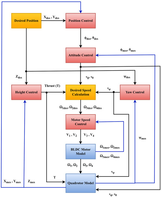
Figure 3. Block diagram of the overall control scheme.

3.1. Height Control

The total thrust force, $T$, which is the sum of an individual rotor’s thrust, controls the quadrotor’s height. We formulate the height control law to regulate the distance from the ground to the quadrotor’s center of mass by deriving it from the state space representation of the quadrotor system in Equation (25).

$$\begin{gathered} {\dot{x}}_5=x_6 \\ {\dot{x}}_6=-g+{\displaystyle \frac{U_{z}T}{m}} \end{gathered}$$

(33)

Step 1: Define tracking error $e_z$ and its derivative ${\dot{e}}_z$ in position $Z$, as follows:

$$\begin{gathered} e_z=x_5-z_{des} \\ {\dot{e}}_z={\dot{x}}_5-{\dot{z}}_{des}=x_6-{\dot{z}}_{des} \end{gathered}$$

(34)

A virtual control of ${\tilde{u}}_1$ and a virtual error $e_{2z}$ are chosen as follows:

$$\begin{gathered} {\tilde{u}}_1={\dot{z}}_{des}-c_z{e}_z \\ {e}_{2z}=x_6-{\tilde{u}}_1=x_6-{\dot{z}}_{des}+c_z{e}_z \end{gathered}$$

(35)

where $c_z$ is a positive constant control parameter, and the error $e_{2z}$ converges to zero as the tracking error $e_z$ also approaches zero. To stabilize the height control system, we define the candidate Lyapunov function $V_{1z}$ using this error:

$$V_{1z}={\displaystyle \frac{1}{2}}{e}_z^2,$$

(36)

Then, the Lyapunov candidate’s time derivative can be represented by

$${\dot{V}}_{1z}=e_z{\dot{e}}_z=e_z(x_6-{\dot{z}}_{des})=e_z{e}_{2z}-c_z{e}_z^2,$$

(37)

If we set $e_{2z}$ = 0, then ${\dot{V}}_{1z}=-c_z{e}_z^2\le 0$, which satisfies the Lyapunov stability criterion. Let us proceed to the next step.

Step 2: Define a switching surface (or sliding surface) ${\delta }_z$ and its derivative ${\dot{\delta }}_z$ as follows:

$$\begin{gathered} {\delta }_z=k_z{e}_z+e_{2z} \\ {\dot{\delta }}_z=k_z{\dot{e}}_z+{\dot{e}}_{2z} \end{gathered}$$

(38)

where $k_z>0$ is chosen to ensure exponential convergence of the tracking error. This ensures fast but non-oscillatory error decay.

And the augmented Lyapunov function $V_{2z}$ is given by

$$V_{2z}=V_{1z}+{\displaystyle \frac{1}{2}}{\delta }_z^2,$$

(39)

Then, the time derivative of $V_{2z}$ is given by

$${\dot{V}}_{2z}={\dot{V}}_{1z}+{\delta }_z{\dot{\delta }}_z,$$

(40)

From Equation (35), ${\dot{e}}_z$ and ${\dot{e}}_{2z}$ are represented as follows:

$$\begin{gathered} {\dot{e}}_z={\dot{e}}_{2z}-c_z{\dot{e}}_z \\ {\dot{e}}_{2z}={\dot{x}}_6-{\dot{\tilde{u}}}_1 \end{gathered}$$

(41)

Substituting Equations (34), (35), and (41) into Equation (40) gives

$$\begin{gathered} {\dot{V}}_{2z}=e_z{e}_{2z}-c_z{e}_z^2+{\delta }_z\left(k_z{\dot{e}}_z+{\dot{e}}_{2z}\right) \\ {\dot{V}}_{2z}=e_z{e}_{2z}-c_z{e}_z^2+{\delta }_z(k_z(e_{2z}-c_z{e}_z)-g+{\displaystyle \frac{U_{z}T}{m}}-{\dot{\tilde{u}}}_1) \end{gathered}$$

(42)

In order to satisfy the Lyapunov stability criterion ${\dot{V}}_{2z}\le 0$, the thrust force control input $T$ is chosen as follows:

$$T=-{\displaystyle \frac{m}{U_z}}\left[(k_z+c_z)(e_{2z}-c_z{e}_z)-g-{\ddot{z}}_{des}+h_z{\delta }_z+{\mu }_{z}sign\left({\delta }_z\right)\right],$$

(43)

where $k_z$, $c_z$, $h_z$, ${\mu }_z$ > 0, and $U_z=\mathrm{c}\mathrm{o}\mathrm{s}\left(\varphi \right)cos\left(\theta \right)$. These parameters are determined based on Lyapunov stability criteria, which guarantee the negative definiteness of ${\dot{V}}_{2z}<0$ and thus ensure system stability. The switching gains ($h_z$, ${\mu }_z$) are chosen to satisfy ${\delta }_z{\dot{\delta }}_z<0$ under the worst-case estimated matched disturbance $D_z$. To guarantee this, switching parameters are set slightly higher than the upper bound of $D_z$, ensuring finite-time convergence to the sliding manifold. Finally, all controller parameters are fine-tuned using a GA, which optimizes the parameters to minimize the tracking error and achieve fast convergence while maintaining robustness.

We can check the stability of the designed controller by substituting Equation (43) into Equation (42):

$$\begin{gathered} {\dot{V}}_{2z}=e_z{e}_{2z}-c_z{e}_z^2+{\delta }_z\left(k_z\left(e_{2z}-c_z{e}_z\right)-g+{\displaystyle \frac{U_{z}T}{m}}-{\dot{\tilde{u}}}_1\right) \\ {\dot{V}}_{2z}=e_z{e}_{2z}-c_z{e}_z^2-h_z{\delta }_z^2-{\mu }_z\left|{\delta }_z\right| \end{gathered}$$

(44)

Since $c_z$, $h_z$, ${\mu }_z$ > 0, thus, if we set $e_{2z}=0$, then the time derivative of the Lyapunov candidate is semi-negative definite, as follows:

$${\dot{V}}_{2z}=-c_z{e}_z^2-h_z{\delta }_z^2-{\mu }_z\left|{\delta }_z\right|\le 0$$

(45)

Thus, the system is asymptotically stable.

3.2. Attitude Control

The rotational (or attitude) subsystem of the quadrotor, comprising the roll, pitch, and yaw angles, is crucial for solving the stabilization and tracking control problems of the quadrotor. From the state space representation of the quadrotor system of Equation (25), we have

$$\begin{gathered} {\dot{x}}_7={\displaystyle \frac{I_{yy}-I_{zz}}{I_{xx}}}{x}_8{x}_9-{\displaystyle \frac{J_r}{I_{xx}}}{x}_8{\Omega }_r+{\displaystyle \frac{1}{I_{xx}}}{\tau }_{\varphi }+D_{\varphi } \\ {\dot{x}}_8={\displaystyle \frac{I_{zz}-I_{xx}}{I_{yy}}}{x}_7{x}_9+{\displaystyle \frac{J_r}{I_{yy}}}{x}_7{\Omega }_r+{\displaystyle \frac{1}{I_{yy}}}{\tau }_{\theta }+D_{\theta } \\ {\dot{x}}_9={\displaystyle \frac{I_{xx}-I_{yy}}{I_{zz}}}{x}_7{x}_8+{\displaystyle \frac{1}{I_{zz}}}{\tau }_{\psi }+D_{\psi } \\ {\dot{x}}_{10}=x_7+x_8\mathit{sin}(x_{10}\left)\mathit{tan}(x_{11}\right)+x_9\mathit{cos}(x_{10}\left)\mathit{tan}(x_{11}\right) \\ {\dot{x}}_{11}=x_8\mathit{cos}(x_{10})-x_9\mathit{sin}(x_{10}) \\ {\dot{x}}_{12}={\displaystyle \frac{x_8\mathit{sin}(x_{10})}{\mathit{cos}(x_{11})}}+{\displaystyle \frac{x_9\mathit{cos}(x_{10})}{\mathit{cos}(x_{11})}} \end{gathered}$$

(46)

We can simplify the control design procedure by defining the states in a matrix format, as follows:

$$X_{Rot}^{Earth}=X_R^E=\left[\begin{array}{c}{x}_{10}\\ x_{11}\\ x_{12}\end{array}\right]=\left[\begin{array}{c}\varphi \\ \theta \\ \psi \end{array}\right],$$

(47)

$$X_{Rot}^{Body}=X_R^B=\left[\begin{array}{c}{x}_7\\ x_8\\ x_9\end{array}\right]=\left[\begin{array}{c}P\\ Q\\ R\end{array}\right]$$

(48)

The updated state space representation for the rotational subsystem is given by

$$\begin{gathered} {\dot{X}}_R^E=\left[\begin{array}{c}\dot{\varphi }\\ \dot{\theta }\\ \dot{\psi }\end{array}\right]=T_M^{-1}\left[\begin{array}{c}P\\ Q\\ R\end{array}\right]=T_M^{-1}{X}_R^B \\ {\dot{X}}_R^B=\left[\begin{array}{c}\dot{P}\\ \dot{Q}\\ \dot{R}\end{array}\right]=\left[\begin{array}{c}{\displaystyle \frac{I_{yy}-I_{zz}}{I_{xx}}}{x}_8{x}_9-{\displaystyle \frac{J_r}{I_{xx}}}{x}_8{\Omega }_r\\ {\displaystyle \frac{I_{zz}-I_{xx}}{I_{yy}}}{x}_7{x}_9+{\displaystyle \frac{J_r}{I_{yy}}}{x}_7{\Omega }_r\\ {\displaystyle \frac{I_{xx}-I_{yy}}{I_{zz}}}{x}_7{x}_8\end{array}\right]+\left[\begin{array}{ccc}{\displaystyle \frac{1}{I_{xx}}}& 0& 0\\ 0& {\displaystyle \frac{1}{I_{yy}}}& 0\\ 0& 0& {\displaystyle \frac{1}{I_{zz}}}\end{array}\right]\left[\begin{array}{c}{\tau }_{\varphi }\\ {\tau }_{\theta }\\ {\tau }_{\psi }\end{array}\right] \\ {\dot{X}}_R^B=A+B{U}_2 \end{gathered}$$

(49)

To begin formulating the attitude controller, we define the rotational tracking error $E_{1R}$ and its derivative ${\dot{E}}_{1R}$, as follows:

$$\begin{gathered} E_{1R}=\left[\begin{array}{c}\varphi \\ \theta \\ \psi \end{array}\right]-\left[\begin{array}{c}{\varphi }_{des}\\ {\theta }_{des}\\ {\psi }_{des}\end{array}\right]=X_R^E-X_{Rdes}^E \\ {\dot{E}}_{1R}=\left[\begin{array}{c}\dot{\varphi }\\ \dot{\theta }\\ \dot{\psi }\end{array}\right]-\left[\begin{array}{c}{\dot{\varphi }}_{des}\\ {\dot{\theta }}_{des}\\ {\dot{\psi }}_{des}\end{array}\right]={\dot{X}}_R^E-{\dot{X}}_{Rdes}^E \end{gathered}$$

(50)

Considering a candidate Lyapunov function of $V_{1R}$ to stabilize the attitude control system as

$$V_{1R}={\displaystyle \frac{1}{2}}{E}_{1R}{E}_{1R}^T,$$

(51)

The time derivative of $V_{1R}$ gives

$$\begin{gathered} {\dot{V}}_{1R}=E_{1R}^T{\dot{E}}_{1R} \\ {\dot{V}}_{1R}=E_{1R}^T\left({\dot{X}}_R^E-{\dot{X}}_{Rdes}^E\right) \end{gathered}$$

(52)

A virtual control of ${\tilde{U}}_2$ and a virtual control error of $E_{2R}$ are chosen, which satisfies the semi-negative definiteness of the candidate Lyapunov function ${\dot{V}}_{1R}$, as follows:

$$\begin{gathered} {\tilde{U}}_2={\dot{X}}_{Rdes}^E-C_R{E}_{1R} \\ {E}_{2R}={\dot{X}}_R^E-{\tilde{U}}_2={\dot{X}}_R^E-{\dot{X}}_{Rdes}^E+C_R{E}_{1R} \end{gathered}$$

(53)

Substituting Equation (53) into Equation (52) gives

$$\begin{gathered} {\dot{V}}_{1R}=E_{1R}^T{\dot{E}}_{1R} \\ {\dot{V}}_{1R}=E_{1R}^T{E}_{2R}-C_R^T{E}_{1R}^2 \end{gathered}$$

(54)

Setting $E_{2R}=0$ results in ${\dot{V}}_{1R}=-C_R^T{E}_{1R}^2$, which satisfies the Lyapunov stability criterion. We can now proceed to the next step by defining a sliding surface ${\delta }_R$ and its derivative ${\dot{\delta }}_R$, as follows:

$$\begin{gathered} {\delta }_R=K_R{E}_{1R}+E_{2R} \\ {\dot{\delta }}_R=K_R{\dot{E}}_{1R}+{\dot{E}}_{2R} \end{gathered}$$

(55)

The augmented Lyapunov function $V_{2R}$ is given by

$$V_{2R}=V_{1R}+{\displaystyle \frac{1}{2}}{\delta }_R{\delta }_R^T$$

(56)

From Equations (51) and (54), we have

$$\begin{gathered} {\dot{E}}_{1R}={\dot{X}}_R^E-{\dot{X}}_{Rdes}^E \\ {\dot{E}}_{1R}=E_{2R}-C_R{E}_{1R} \end{gathered}$$

(57)

The time derivative of $V_{2R}$ yields

$$\begin{gathered} {\dot{V}}_{2R}={\dot{V}}_{1R}+{\delta }_R^T{\dot{\delta }}_R \\ {\dot{V}}_{2R}=E_{1R}^T{E}_{2R}-C_R^T{E}_{1R}^2+{\delta }_R^T\left({\ddot{X}}_R^E+{\ddot{X}}_{Rdes}^E+\left(K_R-C_R\right){\dot{E}}_{1R}\right) \end{gathered}$$

(58)

In order to satisfy the Lyapunov stability criterion ${\dot{V}}_{2R}$, the derivative of sliding surface ${\dot{\delta }}_R$ has to satisfy ${\dot{\delta }}_R\le 0$, which is formulated as follows:

$${\dot{\delta }}_R={\ddot{X}}_R^E+{\ddot{X}}_{Rdes}^E+\left(K_R-C_R\right){\dot{E}}_{1R}=-H_R{\delta }_R-{\beta }_R,$$

(59)

$${\beta }_R=\left[\begin{array}{ccc}{\mu }_{\varphi }& 0& 0\\ 0& {\mu }_{\theta }& 0\\ 0& 0& {\mu }_{\psi }\end{array}\right]\left[\begin{array}{c}sgn\left({\delta }_{\varphi }\right)\\ sgn\left({\delta }_{\theta }\right)\\ sgn\left({\delta }_{\psi }\right)\end{array}\right],$$

(60)

where sgn(·) denotes the signum function. The control input that satisfies Equation (60) can be formulated as follows:

$$\begin{gathered} {\ddot{X}}_R^E+{\ddot{X}}_{Rdes}^E+\left(K_R-C_R\right){\dot{E}}_{1R}=-H_R{\delta }_R-{\beta }_R \\ {U}_2=B^{-1}\left[T_M\left(G_R-{\dot{T}}_M^{-1}{X}_R^B\right)-A\right] \end{gathered}$$

(61)

$C_R$, $K_R$, $H_R$ $\in$ ${\mathbb{R}}^{3\times 3}$ are positive definite diagonal matrices and $G_R$ is given by

$$G_R=-{\ddot{X}}_{Rdes}^E-\left(K_R-C_R\right){\dot{E}}_{1R}-H_R{\delta }_R-{\beta }_R$$

(62)

We can check the stability of the designed controller by substituting Equation (61) into Equation (59):

$$\begin{gathered} {\dot{V}}_{2R}=E_{1R}^T{E}_{2R}-C_R^T{E}_{1R}^2+{\delta }_R^T\left({\ddot{X}}_R^E+{\ddot{X}}_{Rdes}^E+\left(K_R-C_R\right){\dot{E}}_{1R}\right) \\ {\dot{V}}_{2R}=E_{1R}^T{E}_{2R}-C_R^T{E}_{1R}^2-H_R^T{\delta }_R^2-{\delta }_R^T{\beta }_R \end{gathered}$$

(63)

Since $C_R$, $K_R$, and $H_R$ are positive definite diagonal matrices, if we set $E_{2R}=0$, then the time derivative of the Lyapunov candidate is semi-negative definite, as follows:

$${\dot{V}}_{2R}=-C_R^T{E}_{1R}^2-H_R^T{\delta }_R^2-{\delta }_R^T\left|{\beta }_R\right|\le 0$$

(64)

Thus, the system is asymptotically stable.

3.3. Trajectory Control

In trajectory control, we control the quadrotor’s $X$ and $Y$ positions to enable it to effectively follow the desired trajectories. Due to the underactuated nature of the quadrotor system, the $X$ and $Y$ positions cannot be independently controlled. Therefore, we must design virtual control inputs, $U_x$ and $U_y$. By applying a similar procedure to the one used for the rotational subsystem, the control inputs required to stabilize the translational subsystems can be determined as follows:

$$\begin{gathered} T=-{\displaystyle \frac{m}{U_z}}\left[\left(k_z+c_z\right)\left(e_{2z}-c_z{e}_z\right)-g-{\ddot{z}}_{des}+h_z{\delta }_z+{\mu }_{z}sgn\left({\delta }_z\right)\right] \\ {U}_x=-{\displaystyle \frac{m}{T}}\left[\left(k_x+c_x\right)\left(e_{2x}-c_x{e}_x\right)-{\ddot{x}}_{des}+h_x{\delta }_x+{\mu }_{x}sgn\left({\delta }_x\right)\right] \\ {U}_y=-{\displaystyle \frac{m}{T}}\left[(k_y+c_y)(e_{2y}-c_y{e}_y)-{\ddot{y}}_{des}+h_y{\delta }_y+{\mu }_{y}sgn\left({\delta }_y\right)\right] \end{gathered}$$

(65)

where $T$ is the thrust force, which drives the quadrotor up and down, $U_x$ is the virtual control of position $X$, and $U_y$ is the virtual control of position $Y$.

3.4. Tuning of the Controller Parameters

The BSMC for the quadcopter comprises 24 parameters: $k_{\varphi }$, $k_{\theta }$, $k_{\psi }$, $k_x$, $k_y$, $k_z$, $c_{\varphi }$, $c_{\theta }$, $c_{\psi }$, $c_x$, $c_y$, $c_z$, $h_{\varphi }$, $h_{\theta }$, $h_{\psi }$, $h_x$, $h_y$, $h_z$, ${\mu }_{\varphi }$, ${\mu }_{\theta }$, ${\mu }_{\psi }$, ${\mu }_x$, ${\mu }_y$, and ${\mu }_z$. To optimize the performance, its parameters are tuned using a genetic algorithm. This optimization is performed while adhering to the following control input constraints:

$$\begin{gathered} 0\le T\le 4K_T{\Omega }_{max}^2 \\ -K_{T}l{\Omega }_{max}^2\le {\tau }_{\varphi },{\tau }_{\theta }\le K_{T}l{\Omega }_{max}^2 \\ -2K_D{\Omega }_{max}^2\le {\tau }_{\psi }\le 2K_D{\Omega }_{max}^2 \end{gathered}$$

(66)

where ${\Omega }_{max}$ is the maximum speed of the motors (actuators). For optimization, various performance indexes are often used to evaluate system performance; common choices include Integral Squared Error (ISE), Integral Time Squared Error (ITSE), Integral Absolute Error (IAE), and Integral Time Absolute Error (ITAE). In this study, we use the IAE performance index to evaluate the control system performance.

$$IAE={\int }_0^{\infty }\left|e\left(t\right)\right|dt$$

(67)

4. Results and Discussion

To evaluate the effectiveness and stability of the proposed BSMC, we will test it using the quadrotor’s dynamics by running a series of trajectory tracking scenarios to assess the controller’s performance under different conditions. The simulation uses the system parameters from Table 1, which are based on data from the Science and Technology Institute at Adama Science and Technology University and an external reference [39]. To make the test more realistic, the simulation also includes time-varying wind disturbances.

Table 1. Physical parameters of the quadrotor.

Parameters	Value	Unit
Arm length	0.5	m
Moment inertia of the body in the x-axis ($I_{xx}$)	3.8278 × 10−3	Nm/(rad/s2)
Moment inertia of the body in the y-axis ($I_{yy}$)	3.8278 × 10−3	Nm/(rad/s2)
Moment inertia of the body in the z-axis ($I_{zz}$)	7.1345 × 10−4	Nm/(rad/s2)
Moment inertia of the motor ($J_r$)	2.8385 × 10−5	Kg/m2
Total mass of the quadrotor ($m$)	0.5 to 18	Kg
Gravitational acceleration ($g$)	9.81	m/s2
Lift constant ($K_T$)	2.9842 × 10−5	N/(rad/s)
Drag constant ($K_D$)	3.232 × 10−7	Nm/(rad/s)
Maximum speed of the motors (${\Omega }_{max}$)	400$\mathsf{\pi }$	rad/s

To tune the controller’s parameters, a genetic algorithm was used. We used MATLAB R2022b’s ga function with Equation (67) as the objective function to evaluate the performance of each parameter set. The algorithm was configured with a default population size of 50 individuals. The default genetic operators were used: stochastic uniform selection, scattered crossover with a rate of 0.8, and Gaussian mutation with both scale and shrink set to their default value of 1. Because a genetic algorithm is stochastic, its results can vary with each run due to the random initialization of the population and the probabilistic nature of its genetic operators. To ensure more reliable and consistent findings, we performed 20 independent runs and averaged the results. This approach helps to mitigate the impact of random fluctuations. The GA search space was constrained to the interval [0, 100] for all controller parameters. The lower bound of zero guarantees positive controller gains, which are required to preserve stability in the Lyapunov framework, while the upper bound of 100 was chosen based on prior controller tuning experience and to avoid excessively large values that may lead to actuator saturation or numerical instability. Such ranges are consistent with practical UAV control design in the literature.

The optimization process of GA is summarized in Figure 4. The algorithm begins with a randomly generated population, evaluates the fitness of each candidate solution, and iteratively applies selection, crossover, and mutation until the stopping condition is met. This ensures a balance between exploration of the parameter space and exploitation of high-performing solutions.

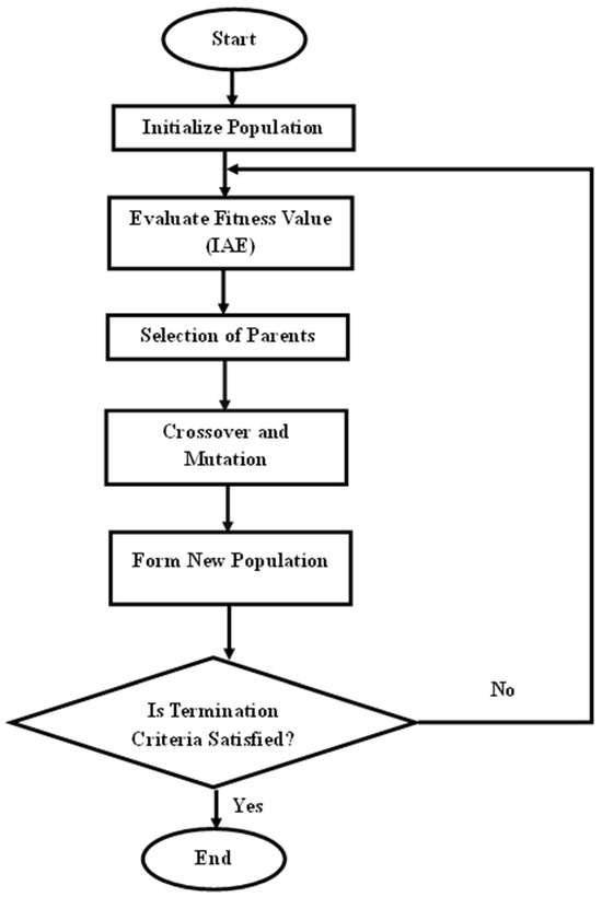
Figure 4. Flowchart of the genetic algorithm.

The results are summarized in Table 2.

Table 2. GA-tuned parameters of the proposed controller.

Parameters	Values	Parameters	Values
$c_{\varphi }$	4.6534	$c_x$	2.5487
$c_{\theta }$	90.3252	$c_y$	1.7297
$c_{\psi }$	46.0854	$c_z$	0.6906
$k_{\varphi }$	80.9636	$k_x$	14.7240
$k_{\theta }$	87.8250	$k_y$	0.1348
$k_{\psi }$	3.7395	$k_z$	62.2074
$h_{\varphi }$	52.8354	$h_x$	2.0858
$h_{\theta }$	86.9526	$h_y$	0
$h_{\psi }$	9.6185	$h_z$	0.7383
${\mu }_{\varphi }$	87.0379	${\mu }_x$	0
${\mu }_{\theta }$	31.0951	${\mu }_y$	3.2361
${\mu }_{\psi }$	86.7513	${\mu }_z$	65.7034

4.1. Simulation Results Under Normal Conditions

In this section, the quadrotor is evaluated on its ability to track a range of predefined trajectories. The simulations are conducted under ideal conditions, with no external disturbances or parametric uncertainties. The position coordinates ($X$, $Y$, $Z$) are recorded in meters, while the Euler angles ($\varphi$, $\theta$, $\psi$) are measured in radians.

4.1.1. Setpoint Tracking Performance at m = 1.5 Kg

Under this tracking problem, the quadrotor is commanded to hover at the position of $X_{des}=2$, $Y_{des}=2$, $Z_{des}=4$, and ${\psi }_{des}=0$. Figure 5a shows the resulting $X$, $Y$, and $Z$ position trajectories. It can be seen from the figure that the quadrotor effectively follows the commanded $X$ and $Y$ position trajectories with a rise time of 1.0656 s and 1.428 s and a settling time of 1.9375 s and 2.226 s, respectively. There is no overshoot in either the $X$ or $Y$ trajectory. Similarly, the quadrotor successfully hovers at the commanded height of 4 m. The $Z$-axis trajectory has a rise time of 1.3767 s and a settling time of 1.7643 s, with an overshoot of 3.79%. Over the simulation, the IAE for each of the $X$, $Y$, and $Z$ position trajectories were calculated using Equation (66), resulting in values of 1.1025, 1.7096, and 2.9337, respectively.

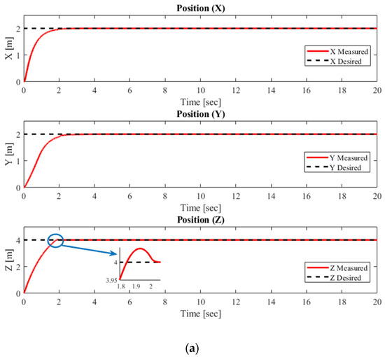
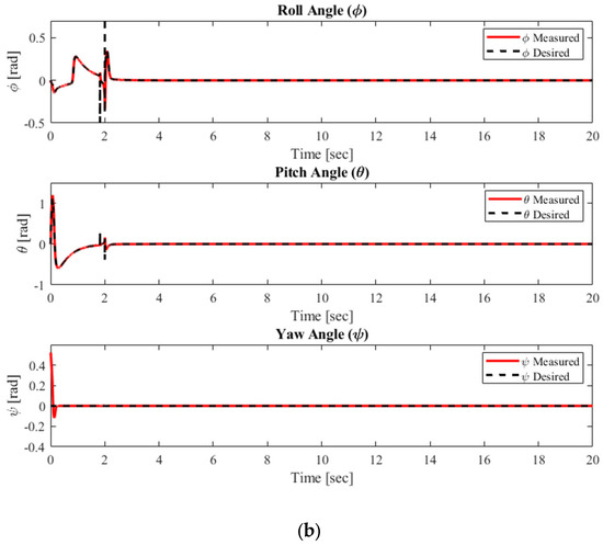
Figure 5. Set point tracking: (a) translational subsystem; (b) rotational subsystem.

Figure 5b illustrates the commanded roll, pitch, and yaw angles corresponding to the desired $Y$ and $X$ positions, respectively. As observed, the quadrotor accurately generates the roll and pitch angles required to achieve the target $Y$ and $X$ positions. Furthermore, the commanded yaw angle is attained within 0.2129 s. Over the simulation period, the integral absolute errors for the roll, pitch, and yaw angles are 0.0207, 0.0220, and 0.0385, respectively.

4.1.2. Circular Trajectory Tracking Performance at m = 1.5 Kg

Under this tracking problem, the quadrotor tracks the trajectory generated by $X_{des}=0.5cos(\pi t/20)$, $Y_{des}=0.5sin(\pi t/20)+0.5$, $Z_{des}=3$, and ${\psi }_{des}=0$. The resulting $X$, $Y$, and $Z$ position trajectories are shown in Figure 6b. It can be seen that the quadrotor effectively tracks the desired $X$ and $Y$ positions with IAEs of 0.2785 and 0.3222, respectively, over the simulation duration. In the vertical axis, the quadrotor maintains the desired altitude of 3 m with a rise time of 1.1855 s, a settling time of 1.5034 s, and an overshoot of 3.80%. The IAE for the altitude ($Z$) is 1.9418.

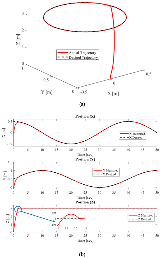
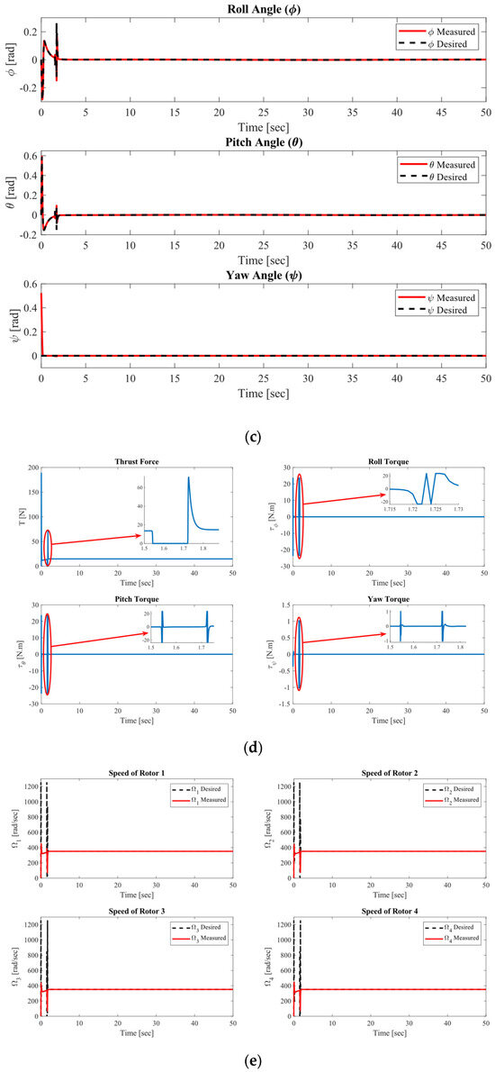
Figure 6. Circular trajectory tracking: (a) 3D view; (b) translational subsystem; (c) rotational subsystem; (d) control inputs; (e) rotor speed.

The corresponding roll and pitch angles, which generate the desired $Y$ and $X$ positions, along with the desired yaw angle, are shown in Figure 6c. The quadrotor precisely produces the roll and pitch responses required to achieve the target $Y$ and $X$ positions, while the desired yaw is reached within 1.9095 s. Over the simulation period, the IAEs for the roll, pitch, and yaw angles are 0.0078, 0.0052, and 0.0386, respectively.

4.1.3. Figure-of-Eight-Shaped Trajectory Tracking Performance at m = 1.5 Kg

Under this tracking problem, the quadrotor tracks the trajectory generated by $X_{des}=cos\left(t\right)$, $Y_{des}=0.5sin\left(2t\right)$, $Z_{des}=2$, and ${\psi }_{des}=0$. The resulting $X$, $Y$, and $Z$ position trajectories are depicted in Figure 7b. The quadrotor accurately follows the desired $X$ and $Y$ positions, with IAEs of 0.5381 and 0.1071, respectively, over the simulation period. In the vertical axis, it maintained an altitude of 2 m, with a rise time of 0.9326 s, a settling time of 1.1721 s, and a maximum overshoot of 3.79%. The IAE for the altitude ($Z$) is 1.0575.

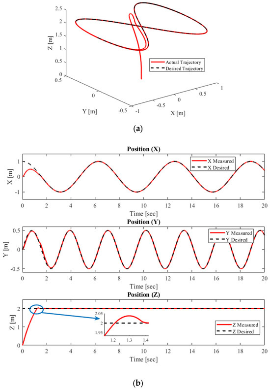
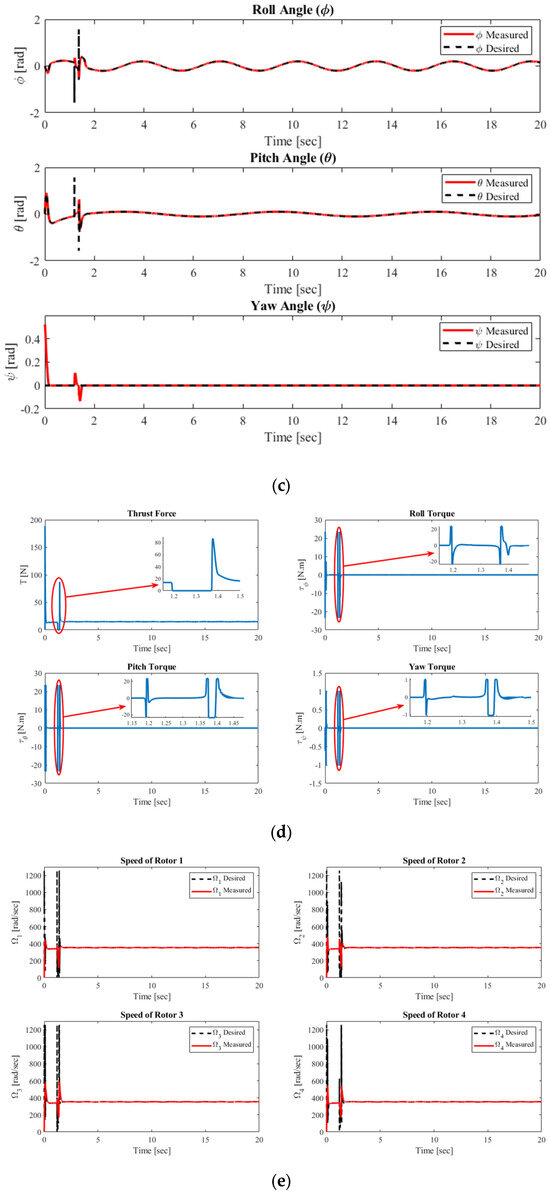
Figure 7. Figure-of-eight-shaped trajectory tracking: (a) 3D view; (b) translational subsystem; (c) rotational subsystem; (d) control inputs; (e) rotor speed.

The corresponding roll and pitch angles, which generate the desired $Y$ and $X$ positions, together with the yaw angle, are shown in Figure 7c. The quadrotor effectively produces the roll and pitch responses required to achieve the target positions, while the commanded yaw is attained within 1.5036 s. Over the simulation period, the integral absolute errors for the roll, pitch, and yaw angles are 0.0419, 0.0394, and 0.0539, respectively.

4.1.4. Complex Helix Trajectory Tracking Performance at m = 1.5 Kg

Under this tracking problem, the quadrotor is commanded to track the trajectory generated by $X_{des}=cos\left(0.05t\right)-{\mathit{cos}}^3\left(0.05t\right)$, $Y_{des}=sin\left(0.05t\right)-{\mathit{sin}}^3\left(0.05t\right)$, $Z_{des}=0.3t$, and ${\psi }_{des}=0$. Figure 8c presents the $X$, $Y$, and $Z$ position trajectories for the ramp altitude case. The quadrotor accurately tracks the desired $X$ and $Y$ positions, with IAEs of 0.0054 and 0.0061, respectively. In the vertical axis, it follows the desired ramp altitude with an IAE of 0.0600.

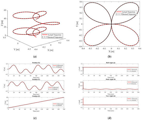
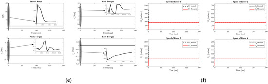
Figure 8. Figure-of-eight-shaped trajectory tracking: (a) 3D view; (b) 2D view; (c) translational subsystem; (d) rotational subsystem; (e) control inputs; (f) motor speed.

The corresponding roll and pitch angles, which generate the desired $Y$ and $X$ positions, together with the yaw angle, are shown in Figure 8d. The quadrotor precisely produces the roll and pitch responses required to achieve the target positions, while the yaw is attained within 0.1691 s. Over the simulation period, the IAEs for the roll, pitch, and yaw Euler angles are 0.0027, 0.0001, and 0.0391, respectively.

4.2. Simulation Result for Quadrotor Subjected to Time-Varying External Disturbance and Parameter Uncertainties

In this section, we evaluate the controller’s robustness and tracking performance and analyze how the controller handles the specified reference trajectory while accounting for parameter uncertainties and external disturbances, which are outlined below.

• We consider parameter uncertainty as a mass variation. This variation is 0.5 Kg to 18 Kg without external disturbances and 0.5 Kg to 12 Kg when the system is subjected to a time-varying external disturbance.
• A time-varying disturbance with a maximum magnitude varying from −2 to +2 in position $X$, from −3 to +3 in position $Y$, and from −5 to +5 in the $Z$ direction is added to the system as a wind disturbance [43]. The quadrotor is assumed to be operating under the influence of the time-varying wind depicted in Figure 9.
  

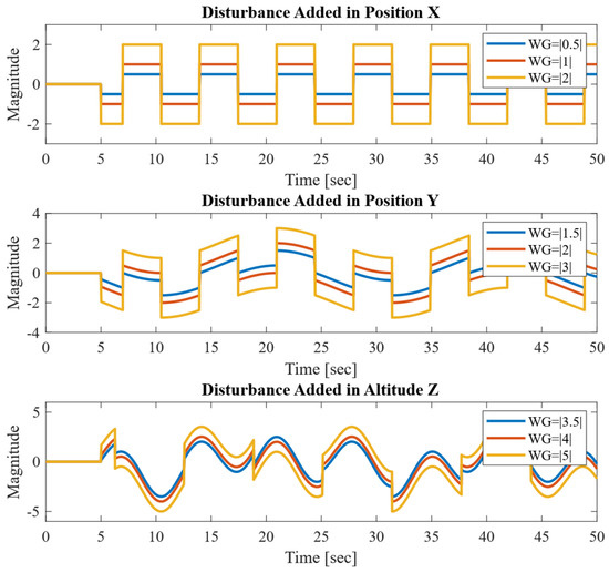  Figure 9. Disturbance added to the system as a wind gust.

The stability analysis assumed matched disturbances, i.e., disturbances entering the system through the same channels as the control inputs. In the experiments, the external wind forces were implemented as bounded time-varying translational disturbances added directly to the translational dynamics: sinusoidal components with amplitudes up to ±2 m/s² in $X$, ±3 m/s² in $Y$, and ±5 m/s² in $Z$, combined with step-like gusts. Since these disturbances enter through the thrust channel, they satisfy the matched disturbance assumption.

4.2.1. Circular Trajectory Tracking Performance for Masses Varying from 0.5 Kg to 18 Kg

The primary source of parametric uncertainty in the quadrotor is mass variation. While the mass is adjusted before take-off and the system signals are configured accordingly, the proposed BSMC controller remains unchanged during operation; it can effectively handle a wide range of quadrotor masses, ranging from 0.5 Kg to 18 Kg.

Figure 10 illustrates the quadrotor’s responses to varying payloads under normal operating conditions, showing that the proposed controller effectively manages mass variations ranging from 0.5 kg to 18 kg. The total IAEs obtained are 2.5846, 3.2951, 4.6648, and 8.2977 for $m$ = 0.5 kg, $m$ = 10 kg, $m$ = 15 kg, and $m$ = 18 kg, respectively. These results are summarized in Table 3.

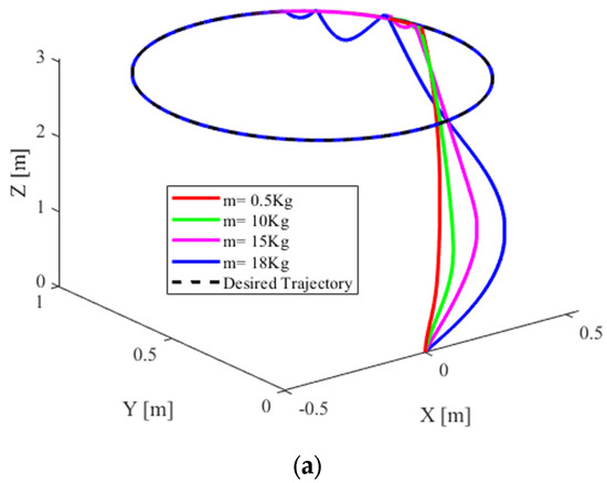
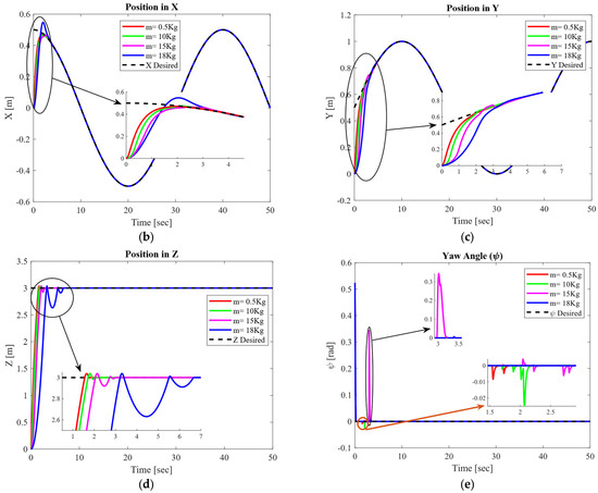
Figure 10. Circular trajectory tracking with a varying total quadrotor mass: (a) 3D view; (b) position $X$; (c) position $Y$; (d) position $Z$; (e) Euler angle $\psi$ (yaw angle).

Table 3. IAE of circular trajectory tracking for quadrotors of different masses.

Mass (kg)	$\mathit{X}$ (m)	$\mathit{Y}$ (m)	$\mathit{Z}$ (m)	$\mathit{\varphi }$ (rad)	$\mathit{\theta }$ (rad)	$\mathit{\psi }$ (rad)
0.5	0.2782	0.3216	1.9333	0.0076	0.0052	0.0387
10	0.3560	0.4588	2.3905	0.0357	0.0140	0.0401
15	0.4511	0.6938	3.3416	0.0802	0.0191	0.0789
18	0.5301	0.9982	6.7203	0.0062	0.0040	0.0390

4.2.2. Circular Trajectory Tracking Performance Under Time-Varying External Disturbance With Different Magnitudes

Figure 11 presents the quadrotor’s responses when subjected to the time-varying disturbances shown in Figure 9. The proposed controller effectively rejects disturbances ranging from −2 to +2 in the $X$ direction, −3 to +3 in the $Y$ direction, and −5 to +5 in the $Z$ direction. The IAEs of the six output variables over the 50 s simulation period are summarized in Table 4.

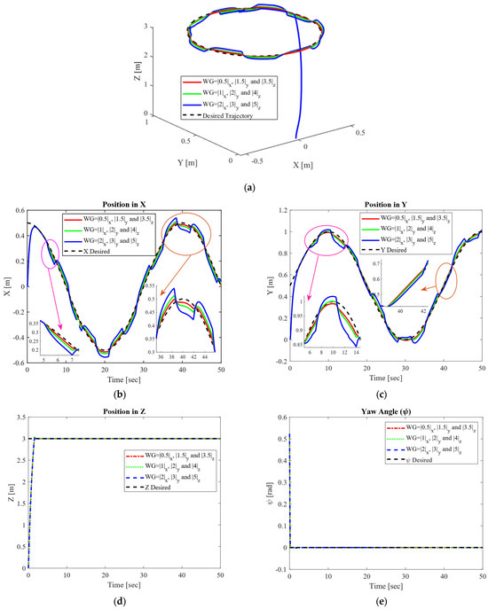
Figure 11. Circular trajectory tracking when the quadrotor is subjected to time-varying disturbance (wind gust): (a) 3D view; (b) position $X$; (c) position $Y$; (d) position $Z$; (e) Euler angle $\psi$ (yaw angle).

Table 4. IAE of circular trajectory tracking when the quadrotor is subjected to wind gusts of different magnitudes.

Bounds of Wind Gusts	$\mathit{X}$ (m)	$\mathit{Y}$ (m)	$\mathit{Z}$ (m)	$\mathit{\varphi }$ (rad)	$\mathit{\theta }$ (rad)	$\mathit{\psi }$ (rad)
$\left|WG\_x\right|$$< 0.5, \left|WG\_y\right|$$< 1.5, \left|WG\_z\right|$ < 3.5	0.7737	0.8445	1.9434	0.0113	0.0070	0.0386
$\left|WG\_x\right|$$< 1, \left|WG\_y\right|$$< 2, \left|WG\_z\right|$ < 4	1.2711	1.0141	1.9435	0.0198	0.0121	0.0387
$\left|WG\_x\right|$$< 2, \left|WG\_y\right|$$< 3, \left|WG\_z\right|$ < 5	2.2655	1.9306	1.9443	0.0502	0.0283	0.0390

4.2.3. Circular Trajectory Tracking Performance Under Time-Varying External Disturbances and Mass Varying from 0.5 Kg to 12 Kg

Under this tracking mode, the quadrotor tracks the trajectory generated by $X_{des}=cos0.5(\pi t/20)$, $Y_{des}=0.5sin(\pi t/20)+0.5$, $Z_{des}=3$, and ${\psi }_{des}=0$, which is a circular shape at a height of 3 m from the ground. Figure 12 shows the quadrotor’s responses under simultaneous payload variations and time-varying external disturbances. The proposed controller successfully manages payload changes from 0.5 kg to 12 kg while compensating for wind disturbances with amplitudes ranging from −2 to +2 in the $X$ direction, −3 to +3 in the $Y$ direction, and −5 to +5 in the $Z$ direction.

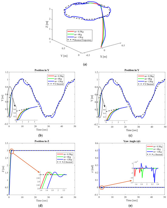
Figure 12. Circular trajectory tracking when the quadrotor is subjected to time-varying disturbance (wind gust) and parameter uncertainties (mass variation): (a) 3D view; (b) position $X$; (c) position $Y$; (d) position $Z$; (e) Euler angle $\psi$ (yaw angle).

In comparison, ref. [27] proposed a hybrid adaptive neural backstepping controller combined with integral fast terminal sliding mode. Their design employs an RBF neural network with online adaptation to approximate lumped uncertainties, which theoretically improves robustness against payload variations by dynamically estimating the effect of mass changes. While this approach is expected to provide stronger compensation for large and rapidly changing payloads without requiring retuning, the proposed BSMC achieves stable tracking across a wide payload range with a simpler structure and without the additional computational burden of neural adaptation. Similarly, ref. [28] developed an adaptive terminal sliding mode controller augmented with an RBF neural network and a barrier Lyapunov-based adaptive gain law. Their method explicitly targets finite-time convergence and includes adaptive mechanisms that automatically adjust controller gains under parametric changes such as mass variation. This makes their controller theoretically well-suited to maintain precise tracking under significant payload changes without manual retuning. In contrast, the proposed BSMC relies on its sliding action and GA-tuned fixed gains for robustness, which may lead to some increase in tracking error under very large payload variations. Nevertheless, our results confirm that the controller maintains stable and accurate performance across a broad payload range, with lower implementation complexity and fewer adaptive components than the RBFNN-based adaptive method.

Overall, these comparisons highlight that while recent adaptive neural or terminal sliding-mode controllers offer strong theoretical compensation for large payload variations, the proposed BSMC achieves a practical balance by ensuring robust performance across a wide load range with reduced structural and computational complexity.

4.3. Comparison of the Proposed Controller with SMC and BSC

Figure 13 shows a comparison of Backstepping Control (BSC), SMC, and the proposed BSMC for circular trajectory tracking under normal operating conditions; it can be observed that the proposed BSMC outperforms both BSC and SMC in circular trajectory tracking. The total IAEs for BSC, SMC, and BSMC are 4.1287, 5.5410, and 2.5941, respectively, demonstrating the superior tracking accuracy of the proposed approach.

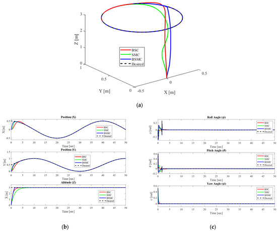
Figure 13. Comparison of BSC, SMC, and BSMC for circular trajectory tracking: (a) 3D view; (b) translational subsystem; (c) rotational subsystem.

Overall, the high tracking accuracy of BSMC is attributed to its hybrid design. The backstepping approach guarantees a smooth, recursive stabilization of each subsystem, avoiding large overshoot, while the sliding mode term provides robustness against matched uncertainties and external disturbances by enforcing finite-time convergence to the sliding manifold. The GA-based gain tuning further minimizes integral error and optimizes transient response. Consequently, BSMC achieves consistently lower IAE, faster settling, and smoother control input compared to SMC and BSC, as confirmed by Figure 10, Figure 11, Figure 12 and Figure 13 and Table 3, Table 4 and Table 5.

Table 5. Comparison of BSC, SMC, and BSMC for a circular trajectory tracking based on IAE.

Controllers	$\mathit{X}$	$\mathit{Y}$	$\mathit{Z}$	$\mathit{\varphi }$	$\mathit{\theta }$	$\mathit{\psi }$
BSC	0.8836	0.8651	2.2646	0.0002	0.0002	0.1150
SMC	0.4619	0.4508	4.3914	0.0789	0.0783	0.0797
BSMC	0.2785	0.3222	1.9418	0.0078	0.0052	0.0386

Table 5 highlights the overall superiority of BSMC, achieving faster settling times and smoother control effort. The GA-based tuning ensures that the gains are chosen to balance speed of response with control smoothness, reducing chattering and avoiding excessive control energy.

4.4. Performance of SMC Under Varying Loads

Figure 14a illustrates SMC’s performance for payloads of 1.5 kg and 12 kg, which indicates that SMC is unable to handle a payload of 12 kg under normal operating conditions. Figure 14b presents the control input of the SMC, which exhibits the well-known chattering phenomenon, leading to undesirable vibrations and potential heating in the system.

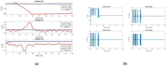
Figure 14. Performance of SMC under varying mass: (a) response of the translational subsystem; (b) control inputs.

5. Conclusions

This study introduced a Backstepping Sliding Mode Control (BSMC) strategy for quadrotor UAV trajectory tracking, addressing a gap in the existing literature. The nonlinear quadrotor dynamics were modeled using the Newton–Euler method, and comparative simulations with BSMC, SMC, and BSC under varying trajectories, payloads, and time-varying disturbances demonstrate that BSMC achieves superior position, altitude, and attitude control. Notably, the proposed approach minimizes chattering in the control inputs, enhancing actuator reliability. These results highlight BSMC as a robust and effective solution for practical QUAV control applications. The comparison with its constituent controllers highlights that BSMC achieves the desired performance improvement with minimal complexity. Although several advanced methods exist, the proposed approach provides a favorable trade-off between robustness, performance, and real-time implementation.

However, this research is limited to simulation studies and does not incorporate hardware implementation or real-world uncertainties such as sensor noise and communication delays. The quadrotor model also assumes idealized aerodynamics and neglects factors like ground effect.

Future work will focus on experimental validation using a real quadrotor platform, extending the control design to handle more complex aerodynamic effects and sensor noises, and integrating adaptive or data-driven elements for online parameter estimation. Also, investigating cooperative control for multi-UAV systems and testing under outdoor flight conditions will further demonstrate the robustness and scalability of the proposed method.

References

- Anitha, V.R.; Shyni, G.; Mythili, C.; Binoj, J.S. Quadcopter Drone for Surveillance, Monitoring and Emergency Medicine Delivery. Proc. Conf. AIP 2025, 3137, 020044. [Google Scholar] [CrossRef]
- Harisankar, R.; Kaushik, A.; Muni, S.S. Path planning for multi-quadrotor 3D boundary surveillance using non-autonomous discrete memristor hyperchaotic system. Frankl. Open 2025, 10, 100239. [Google Scholar] [CrossRef]
- Lyu, M.; Zhao, Y.; Huang, C.; Huang, H. Unmanned Aerial Vehicles for Search and Rescue: A Survey. Remote Sens. 2023, 15, 3266. [Google Scholar] [CrossRef]
- Shope, J.J. Design and Simulation of an AI-Powered Autonomous Quadrotor Framework for Search and Rescue Operations. Master’s Thesis, West Virginia University, Morgantown, WV, USA, 2025. [Google Scholar] [CrossRef]
- Ciccone, F.; Ceruti, A. Real-Time Search and Rescue with Drones: A Deep Learning Approach for Small-Object Detection Based on YOLO. Drones 2025, 9, 514. [Google Scholar] [CrossRef]
- Yeom, S. Thermal Image Tracking for Search and Rescue Missions with a Drone. Drones 2024, 8, 20053. [Google Scholar] [CrossRef]
- ALee, J.; Song, W.; Yu, B.; Choi, D.; Tirtawardhana, C.; Myung, H. Survey of robotics technologies for civil infrastructure inspection. J. Infrastruct. Intell. Resil. 2023, 2, 100018. [Google Scholar] [CrossRef]
- Jacobsen, R.H.; Matlekovic, L.; Shi, L.; Malle, N.; Ayoub, N.; Hageman, K.; Hansen, S.; Nyboe, F.F.; Ebeid, E. Design of an Autonomous Cooperative Drone Swarm for Inspections of Safety Critical Infrastructure. Appl. Sci. 2023, 13, 1256. [Google Scholar] [CrossRef]
- Ravoory, S.; Eggert, C.A.; Balchanos, M.; Mavris, D. Unmanned aerial system-based tactical operations for supporting emergency response in campus communities. In Proceedings of the AIAA Scitech 2021 Forum, Virtual, 11–15 and 19–21 January 2021; pp. 1–16. [Google Scholar]
- Huang, T.; Li, T. Attitude tracking control of a quadrotor UAV subject to external disturbance with L2 performance. Nonlinear Dyn. 2023, 111, 10183–10200. [Google Scholar] [CrossRef]
- Wang, J.; Alattas, K.A.; Bouteraa, Y.; Mofid, O.; Mobayen, S. Adaptive finite-time backstepping control tracker for quadrotor UAV with model uncertainty and external disturbance. Aerosp. Sci. Technol. 2023, 133, 108088. [Google Scholar] [CrossRef]
- Mofid, O.; Mobayen, S. Robust fractional-order sliding mode tracker for quad-rotor UAVs: Event-triggered adaptive backstepping approach under disturbance and uncertainty. Aerosp. Sci. Technol. 2024, 146, 108916. [Google Scholar] [CrossRef]
- Wang, L.; Cheng, Y.; Jiang, B.; Zhang, Y.; Zhu, J.; Tan, X. Adaptability Study of an Unmanned Aerial Vehicle Actuator Fault Detection Model for Different Task Scenarios. Drones 2025, 9, 360. [Google Scholar] [CrossRef]
- Yadav, L.B.; Ghosh, A. Quadcopter Trajectory Tracking Control Analysis by Using PID and LQR Controllers. In International Conference on Systems and Technologies for Smart Agriculture. CISCON 2023, Manipal, India, 6–7 October 2023; Springer Proceedings in Information and Communication Technologies; Springer: Singapore, 2024; pp. 647–657. [Google Scholar] [CrossRef]
- Komiyama, S.; Uchiyama, K.; Masuda, K. Combined Robust Control for Quadrotor UAV Using Model Predictive Control and Super-Twisting Algorithm. Drones 2025, 9, 576. [Google Scholar] [CrossRef]
- Ihnak, M.S.A.; Edardar, M.M. Comparing LQR and PID Controllers for Quadcopter Control Effectiveness and Cost Analysis. In Proceedings of the 2023 IEEE 11th International Conference on Systems and Control, ICSC 2023, Sousse, Tunisia, 18–20 December 2023; pp. 754–759. [Google Scholar] [CrossRef]
- Ahmed, N.; Alrasheedi, N. Commanded Filter-Based Robust Model Reference Adaptive Control for Quadrotor UAV with State Estimation Subject to Disturbances. Drones 2025, 9, 181. [Google Scholar] [CrossRef]
- Xian, W.; Qi, Q.; Liu, W.; Liu, Y.; Li, D.; Wang, Y. Control of quadrotor robot via optimized nonlinear type-2 fuzzy fractional PID with fractional filter: Theory and experiment. Aerosp. Sci. Technol. 2014, 151, 109286. [Google Scholar] [CrossRef]
- Abdulkareem, A.; Oguntosin, V.; Popoola, O.M.; Idowu, A.A. Modeling and Nonlinear Control of a Quadcopter for Stabilization and Trajectory Tracking. J. Eng. 2022, 2022, 2449901. [Google Scholar] [CrossRef]
- Huang, X.; Liu, G.; Liu, Y. Collision Detection and Recovery Control of Drones Using Onboard Inertial Measurement Unit. Drones 2025, 9, 380. [Google Scholar] [CrossRef]
- Hu, Q.; Feng, Y.; Wu, L.; Xi, B. A Nonlinear Adaptive Autopilot for Unmanned Aerial Vehicles Based on the Extension of Regression Matrix. Drones 2023, 7, 275. [Google Scholar] [CrossRef]
- Taame, A.; Lachkar, I.; Abouloifa, A.; Mouchrif, I.; El Aroudi, A. Nonlinear Output Feedback Control for Parrot Mambo UAV: Robust Complex Structure Design and Experimental Validation. Appl. Syst. Innov. 2025, 8, 95. [Google Scholar] [CrossRef]
- Baek, J.; Kang, M. A Synthesized Sliding-Mode Control for Attitude Trajectory Tracking of Quadrotor UAV Systems. IEEE/ASME Trans. Mechatron. 2023, 28, 2189–2199. [Google Scholar] [CrossRef]
- Saif, A.W.A.; Gaufan, K.B.; El-Ferik, S.; Al-Dhaifallah, M. Fractional Order Sliding Mode Control of Quadrotor Based on Fractional Order Model. IEEE Access 2023, 11, 79823–79837. [Google Scholar] [CrossRef]
- Yogi, S.C.; Behera, L.; Nahavandi, S. Adaptive Intelligent Minimum Parameter Singularity Free Sliding Mode Controller Design for Quadrotor. IEEE Trans. Autom. Sci. Eng. 2024, 21, 1805–1823. [Google Scholar] [CrossRef]
- Ahmadi, K.; Asadi, D.; Merheb, A.; Nabavi-Chashmi, S.Y.; Tutsoy, O. Active fault-tolerant control of quadrotor UAVs with nonlinear observer-based sliding mode control validated through hardware in the loop experiments. Control Eng. Pr. 2023, 137, 105557. [Google Scholar] [CrossRef]
- Zhu, J.; Long, X.; Yuan, Q. Adaptive Terminal Sliding Mode Control for a Quadrotor System with Barrier Function Switching Law. Mathematics 2025, 13, 1344. [Google Scholar] [CrossRef]
- Maaruf, M.; Hamanah, W.M.; Abido, M.A. Hybrid Backstepping Control of a Quadrotor Using a Radial Basis Function Neural Network. Mathematics 2023, 11, 991. [Google Scholar] [CrossRef]
- Borbolla-Burillo, P.; Sotelo, D.; Frye, M.; Garza-Castañón, L.E.; Juárez-Moreno, L.; Sotelo, C. Design and Real-Time Implementation of a Cascaded Model Predictive Control Architecture for Unmanned Aerial Vehicles. Mathematics 2024, 12, 739. [Google Scholar] [CrossRef]
- Imran, I.H.; Alyazidi, N.M.; Eltayeb, A.; Ahmed, G. Robust Adaptive Fault-Tolerant Control of Quadrotor Unmanned Aerial Vehicles. Mathematics 2024, 12, 1767. [Google Scholar] [CrossRef]
- Borja-Jaimes, V.; Coronel-Escamilla, A.; Escobar-Jiménez, R.F.; Adam-Medina, M.; Guerrero-Ramírez, G.V.; Sánchez-Coronado, E.M.; García-Morales, J. Fractional-Order Sliding Mode Observer for Actuator Fault Estimation in a Quadrotor UAV. Mathematics 2024, 12, 1247. [Google Scholar] [CrossRef]
- Kapnopoulos, A.; Kazakidis, C.; Alexandridis, A. Quadrotor trajectory tracking based on backstepping control and radial basis function neural networks. Results Control Optim. 2024, 14, 100335. [Google Scholar] [CrossRef]
- Nettari, Y.; Labbadi, M.; Kurt, S. Adaptive Backstepping Integral Sliding Mode Control Combined with Super-Twisting Algorithm for Nonlinear UAV Quadrotor System. IFAC-Pap. 2022, 55, 264–269. [Google Scholar] [CrossRef]
- Nettari, Y.; Kurt, S.; Labbadi, M. Adaptive Robust Control based on Backstepping Sliding Mode techniques for Quadrotor UAV under external disturbances. IFAC-Pap. 2022, 55, 252–257. [Google Scholar] [CrossRef]
- Hou, Y.; Chen, D.; Yang, S. Adaptive Robust Trajectory Tracking Controller for a Quadrotor UAV With Uncertain Environment Parameters Based on Backstepping Sliding Mode Method. IEEE Trans. Autom. Sci. Eng. 2025, 22, 4446–4456. [Google Scholar] [CrossRef]
- Maaruf, M.; Abubakar, A.N.; Gulzar, M.M. Adaptive backstepping and sliding mode control of a quadrotor. J. Braz. Soc. Mech. Sci. Eng. 2024, 46, 1–15. [Google Scholar] [CrossRef]
- Wang, H.; Li, N.; Wang, Y.; Su, B. Backstepping Sliding Mode Trajectory Tracking via Extended State Observer for Quadrotors with Wind Disturbance. Int. J. Control Autom. Syst. 2021, 19, 3273–3284. [Google Scholar] [CrossRef]
- Tsai, S.-H.; Chang, Y.P.; Lin, H.Y.; Chang, L.M. Design and implementation of integral backstepping sliding mode control for quadrotor trajectory tracking. Processes 2021, 9, 1951. [Google Scholar] [CrossRef]
- Belsty, D. Particle Swarm Optimization Tuned Fractional Order Sliding Mode Controller for Altitude Stabilization and Trajectory Tracking of Agricultural Monitoring Quadcopter; Addis Ababa University: Ababa, Ethiopia, 2021; Available online: https://etd.aau.edu.et/items/ea739a2b-2ac2-4753-8fb6-c099fbe4e9cd (accessed on 15 August 2025).
- Luukkonen, T. Modelling and Control of Quadcopter; Aalto University Finland: Espoo, Finland, 2014; Available online: https://sal.aalto.fi/publications/pdf-files/eluu11_public.pdf (accessed on 7 August 2025).
- Alderete, T.S. Simulator Aero Model Implementation; NASA Ames Research Center: Moffett Field, CA, USA, 1995; Available online: https://aethercosmology.com/uploads/short-url/rBEb7fKKTz0TCW5RpEDSOFPmQyl (accessed on 7 August 2025).
- Chovancová, A.; Fico, T.; Chovanec, L.; Hubinský, P. Mathematical modelling and parameter identification of quadrotor (a survey). In Procedia Engineering; Elsevier Ltd.: Amsterdam, The Netherlands, 2014; pp. 172–181. [Google Scholar] [CrossRef]
- Liu, L.; Liu, J.; Li, J.; Ji, Y.; Song, Y.; Xu, L.; Niu, W. Fault-Tolerant Control for Quadrotor Based on Fixed-Time ESO. Mathematics 2022, 10, 4386. [Google Scholar] [CrossRef]
Disclaimer/Publisher’s Note: The statements, opinions and data contained in all publications are solely those of the individual author(s) and contributor(s) and not of MDPI and/or the editor(s). MDPI and/or the editor(s) disclaim responsibility for any injury to people or property resulting from any ideas, methods, instructions or products referred to in the content. |
© 2025 by the authors. Licensee MDPI, Basel, Switzerland. This article is an open access article distributed under the terms and conditions of the Creative Commons Attribution (CC BY) license (https://creativecommons.org/licenses/by/4.0/).