Statistical Evaluation of Beta-Binomial Probability Law for Removal in Progressive First-Failure Censoring and Its Applications to Three Cancer Cases

Abstract

Progressive first-failure censoring is a flexible and cost-efficient strategy that captures real-world testing scenarios where only the first failure is observed at each stage while randomly removing remaining units, making it ideal for biomedical and reliability studies. By applying the $\alpha$-power transformation to the exponential baseline, the proposed model introduces an additional flexibility parameter that enriches the family of lifetime distributions, enabling it to better capture varying failure rates and diverse hazard rate behaviors commonly observed in biomedical data, thus extending the classical exponential model. This study develops a novel computational framework for analyzing an $\alpha$-powered exponential model under beta-binomial random removals within the proposed censoring test. To address the inherent complexity of the likelihood function arising from simultaneous random removals and progressive censoring, we derive closed-form expressions for the likelihood, survival, and hazard functions and propose efficient estimation strategies based on both maximum likelihood and Bayesian inference. For the Bayesian approach, gamma and beta priors are adopted, and a tailored Metropolis–Hastings algorithm is implemented to approximate posterior distributions under symmetric and asymmetric loss functions. To evaluate the empirical performance of the proposed estimators, extensive Monte Carlo simulations are conducted, examining bias, mean squared error, and credible interval coverage under varying censoring levels and removal probabilities. Furthermore, the practical utility of the model is illustrated through three oncological datasets, including multiple myeloma, lung cancer, and breast cancer patients, demonstrating superior goodness of fit and predictive reliability compared to traditional models. The results show that the proposed lifespan model, under the beta-binomial probability law and within the examined censoring mechanism, offers a flexible and computationally tractable framework for reliability and biomedical survival analysis, providing new insights into censored data structures with random withdrawals.

1. Introduction

Progressive first-failure censoring (P-FFC), introduced by Wu and Kuş [1], was developed to address practical challenges in life-testing and reliability studies, where recording every failure time can be prohibitively expensive, time-consuming, or logistically impractical. This scheme integrates two well-known censoring mechanisms: the first-failure censoring design of Balasooriya [2] and the Type-II progressive censoring (TIIPC) framework described by Balakrishnan and Cramer [3]. Unlike conventional methods that observe all failure times, P-FFC records only the earliest failure within each group. This greatly reduces data collection effort while retaining sufficient information for reliable inference. Conceptually, it can be viewed as an adaptation of TIIPC to situations where only the minimum failure time from each group is observed. This design is particularly attractive for applied settings—such as biomedical or reliability experiments—where tracking every failure is infeasible, but recording first failures remains manageable. By focusing on early failures, the scheme achieves a balance between experimental efficiency and statistical reliability.

Wu and Kuş [1] illustrated its practicality using the Weibull lifetime model as an example. Under the P-FFC setup, n independent groups are formed, each containing m identical test units, yielding a total of $n^{★}=n\times m$ units. At each observed failure time, only the first failure within the active group is recorded. After this event, a specified number of groups, $\mathbf{R}=(R_1,R_2,\dots ,R_k)$, are randomly removed from the experiment, in addition to the group where the failure occurred. This process continues until a predetermined number of failures, k$(k\le n)$, is observed. For example, when the first failure $Y_{1:k:n}$ occurs, the affected group plus $R_1$ additional groups are removed, leaving $n-R_1-1$ groups under observation. Similarly, when the second failure $Y_{2:k:n}$ is observed, its corresponding group and $R_2$ additional groups are removed, reducing the number of groups to $n-{\sum }_{i=1}^2{R}_i-2$. This continues until the k-th failure $Y_{k:k:n}$, after which the remaining groups $R_k$ and the group containing the k-th failure are removed. Although this scheme improves experimental efficiency, it assumes that the number of groups removed at each step under the TIIPC design is fixed and known in advance—an assumption that may not hold in real-world experiments. For example, in a clinical trial, after the first patient death, some participants may voluntarily withdraw due to fear or loss of confidence in the treatment. Subsequent deaths may trigger further withdrawals, causing deviations from the planned censoring schedule. While the study may still terminate after observing k failures, the actual number of removals at each stage becomes random and unpredictable. To address this limitation, several extensions of P-FFC have been proposed to incorporate stochastic removal mechanisms. Examples include discrete uniform removals (Huang and Wu [4]), binomial removals (Ashour et al. [5]), and beta-binomial (BB) removals (Elshahhat et al. [6]). These random-removal schemes better capture the inherent uncertainty in withdrawals or unit eliminations encountered in practical testing scenarios. Section 2 provides a detailed explanation of the sampling process under P-FFC with BB-based removals (denoted P-FFC-BB).

The alpha-power transformation technique, proposed by Mahdavi and Kundu [7], offers a systematic and flexible mechanism for constructing new families of probability distributions from a given baseline model. By introducing an additional shape parameter $\alpha$, this transformation enhances skewness, improves tail behavior, and increases modeling flexibility while preserving mathematical tractability. One member of this transformation is the $\alpha$-power exponential (APE) distribution, which generalizes the classical exponential model while maintaining closed-form expressions for both of its characteristic functions. Let Y denote the lifetime of a test unit that follows the two-parameter APE$\left(\mathit{\vartheta }\right)$ distribution, where $\mathit{\vartheta }={(\alpha ,\delta )}^{\top }$. Subsequently, the probability density function (PDF) $g(·)$, cumulative distribution function (CDF) $G(·)$, reliability function (RF) $R(·)$, and hazard rate function (HRF) $h(·)$, evaluated at a mission time $x(>0)$, are expressed as follows:

$$\begin{array}{cc}\hfill & g(y;\mathit{\vartheta })={\displaystyle \frac{\log \left(\alpha \right)\delta e^{-\delta y}{\alpha }^{1-e^{-\delta y}}}{\alpha -1}},y>0,\alpha \ne 1,\hfill \end{array}$$

(1)

$$\begin{array}{cc}\hfill & G(y;\mathit{\vartheta })={\displaystyle \frac{1}{\alpha -1}}\left({\alpha }^{1-e^{-\delta y}}-1\right),\hfill \end{array}$$

(2)

$$\begin{array}{cc}\hfill & R(x;\mathit{\vartheta })={\displaystyle \frac{\alpha }{\alpha -1}}\left(1-{\alpha }^{-e^{-\delta x}}\right),x>0,\hfill \\ \hfill & \mathrm{and}\hfill \end{array}$$

(3)

$$\begin{array}{cc}\hfill & h(x;\mathit{\vartheta })={\displaystyle \frac{\delta \log \left(\alpha \right)e^{-\delta x}}{{\alpha }^{e^{-\delta x}}-1}},\hfill \end{array}$$

(4)

respectively, where $\delta >0$ (scale) and $\alpha >0$ (shape).

The APE distribution extends the classical exponential model by introducing a shape parameter that captures diverse hazard rate patterns, including increasing, decreasing, and bathtub shapes (see Figure 1a). It enhances skewness and tail flexibility while retaining closed-form density and distribution functions, ensuring mathematical simplicity (see Figure 1b). Consequently, it has gained significant attention in reliability analysis, lifetime modeling, and survival studies due to its ability to represent a broad spectrum of hazard rate shapes; see, for example, Salah [8] based on TIIPC; Salah et al. [9] based on Type-II hybrid; Alotaibi et al. [10] based on adaptive TIIPC (ATIIPC); Elbatal et al. [11] based on improved ATIIPC (IATIIPC); and Elsherpieny and Abdel- Hakim [12] based on unified hybrid, among others.

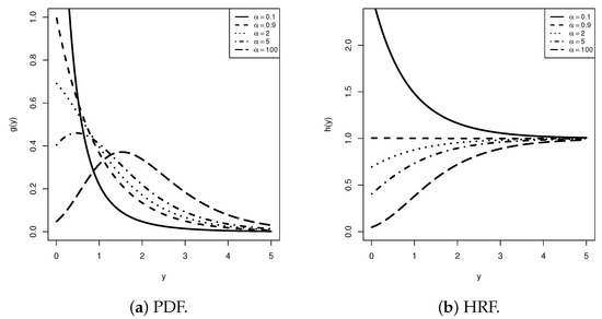
Figure 1. Several shapes for the APE density and failure rate (when $\delta =1$).

Existing alpha-power distributions offer flexibility but are mostly limited to fixed censoring schemes and have not been developed for complex random removal mechanisms such as the beta-binomial structure. The proposed APE–P-FFC-BB strategy provides closed-form likelihoods and a Bayesian inference framework, improving computational tractability under heavy censoring. This extension fills a gap in biomedical applications by enabling practical analysis of oncology data collected through the P-FFC framework.

Recall that the P-FFC plan assumes fixed or deterministic removal schemes, which may not capture the inherent uncertainty in real clinical environments. To overcome this disadvantage, P-FFC-BB was introduced to offer an efficient compromise by recording only the earliest failures from each group while randomly removing unobserved groups to reduce experimental burden. Moreover, the exponential distribution—although widely used due to its simplicity—often lacks the flexibility required to model heterogeneous survival patterns. To address these limitations, this study integrates the alpha-powering transformation of the exponential model, which enhances its shape flexibility, with a BB random removal mechanism under a P-FFC plan. This censoring strategy provides a more realistic and computationally tractable model for analyzing survival data from heterogeneous cancer populations, offering deeper insights into early-failure behavior under complex removal dynamics. Despite the APE model’s flexibility and practical utility, which have been discussed and applied in several life-testing scenarios in the literature, further investigation is warranted in the presence of samples gathered by the proposed censoring mechanism. To address this gap, we summarize the study objectives sixfold as follows:

• Applying the alpha-powering transformation of the exponential distribution within the proposed censoring scheme, adding flexibility to model various hazard rate shapes for biomedical survival data.
• The joint likelihood under such a censoring setup is derived, and both maximum likelihood and Bayesian estimation procedures are developed for the model parameters and key reliability metrics of the APE distribution, as well as of the BB parameters.
• Bayesian estimation of the same unknown parameters is performed under the assumption of independent gamma and beta priors. The analysis is carried out using both symmetric (squared error) and asymmetric (generalized entropy) loss functions, with the Markov Chain Monte Carlo (MCMC) method employed to approximate the posterior distributions.
• In the interval estimation setup, two types of asymptotic confidence intervals and two Bayesian credible intervals are constructed for all model parameters.
• Extensive Monte Carlo simulations are conducted to assess the performance of the estimators under varying test conditions using several precision metrics.
• Three survival datasets—myeloma, lung, and breast cancer—are analyzed to demonstrate the suitability of the proposed model and its applicability to real-world scenarios.

This work primarily develops maximum likelihood and Bayesian estimation under the P-FFC-BB framework, and alternative inferential approaches such as penalized likelihood, EM-type algorithms, or nonparametric Bayesian methods were not explored but may further enhance robustness. Future research could investigate these estimation strategies, particularly for small or highly censored samples, to complement the inference methods presented here.

The remaining sections of this work are arranged as follows: Section 2 depicts the P-FFC-BB design. Section 3 and Section 4 introduce the ML estimators (MLEs) and Bayes estimators, respectively. Section 5 reports the simulation outcomes. Section 6 analyzes the survival times of leukemia and breast cancer patients. Section 7 ultimately concludes the study.

2. The P-FFC-BB Plan

Let $\mathbf{y}=\left\{(y_{1:k:n},r_1),(y_{2:k:n},r_2),\dots ,(y_{k:k:n},r_k)\right\}$ denote the set of observed independent order statistics failure times together with their associated removals collected under the P-FFC-BB removal plan. Assume that the individual lifetimes in $\mathbf{y}$ follow a continuous distribution with PDF ($g(·)$) and CDF ($G(·)$); then, the likelihood function (LF) of the observed data, where $y_i\equiv y_{i:k:n}$, for simplicity, can be expressed as

$${\mathbb{L}}_1\left(\mathsf{\Lambda }|\mathbf{r},\mathbf{y}\right)={\mathbb{C}}_1{m}^k\prod _{i=1}^{k}g\left(y_i;\mathsf{\Lambda }\right){\left[R\left(y_i;\mathsf{\Lambda }\right)\right]}^{m_i^{★}},$$

(5)

where ${\mathbb{C}}_1=n\left(n-r_1-1\right)\cdots \left(n-{\sum }_{i=1}^{k-1}\left(r_i+1\right)\right)$ and $m_i^{★}=m\left(r_i+1\right)-1$.

Suppose that, at the ith observed failure ($i=1,2,\dots ,k-1$), the number of groups removed, denoted by $r_i$, follows a binomial distribution with parameters $n-k-{\sum }_{j=1}^{i-1}{r}_j$ and success probability p. Then, the corresponding probability mass function (PMF) of $r_i$ is

$$Pr\left(\left.\mathbf{R}=\mathbf{r}\right|p\right)=\left({\displaystyle \genfrac{}{}{0pt}{}{n^{*}}{r_i}}\right)p^{r_i}{(1-p)}^{n^{*}-r_i}, i=1,2,\dots ,k-1,$$

(6)

where $n^{*}=n-k-{\sum }_{j=1}^{i-1}{r}_j$, $0⩽r_1⩽n-k$, and $0⩽r_i⩽n^{*}$ for $i=2,3,\dots ,k-1$.

Now, assume that the removal probability p is not constant during the experiment but is, instead, treated as a random variable following a $\mathrm{Beta}\left(\mathit{\lambda }\right)$ distribution, where $\mathit{\lambda }={({\lambda }_1,{\lambda }_2)}^{\top }$. The corresponding beta density function of p is then given by

$$g\left(\left.p\right|\mathit{\lambda }\right)={\displaystyle \frac{1}{B\left({\lambda }_1,{\lambda }_2\right)}}{p}^{{\lambda }_1-1}{(1-p)}^{{\lambda }_2-1},{\lambda }_i>0,i=1,2,0<p<1,$$

(7)

where $B\left({\lambda }_1,{\lambda }_2\right)=\Gamma \left({\lambda }_1\right)\Gamma \left({\lambda }_2\right)/\phantom{\Gamma \left({\lambda }_1\right)\Gamma \left({\lambda }_2\right)\left(\Gamma \left({\lambda }_1+{\lambda }_2\right)\right)}\left(\Gamma \left({\lambda }_1+{\lambda }_2\right)\right)$ is the beta function; see Singh et al. [13] for additional details. Thus, from (6) and (7), the unconditional distribution of $R_i^{\prime }s$ becomes

$$Pr\left(\left.\mathbf{R}=\mathbf{r}\right|\mathit{\lambda }\right)={\displaystyle \frac{1}{B\left({\lambda }_1,{\lambda }_2\right)}}\left({\displaystyle \genfrac{}{}{0pt}{}{n^{*}}{r_i}}\right){\int }_0^1{p}^{{\lambda }_1+r_i-1}{(1-p)}^{{\lambda }_1+n^{*}-r_i-1}dp.$$

After simplifying, we get

$$Pr\left(\left.\mathbf{R}=\mathbf{r}\right|\mathit{\lambda }\right)=\left({\displaystyle \genfrac{}{}{0pt}{}{n^{*}}{r_i}}\right){\displaystyle \frac{B\left({\lambda }_1+r_i,{\lambda }_2+n^{*}-r_i\right)}{B\left({\lambda }_1,{\lambda }_2\right)}}·$$

(8)

The PMF in (8) corresponds to the BB distribution, denoted by $BB(a^{★},{\lambda }_1,{\lambda }_2)$, where $a^{★}$ represents the total number of trials. Accordingly, the joint probability distribution of the BB removals can be written as

$$\begin{array}{cc}{\mathbb{L}}_2\left(\left.\mathbf{R}=\mathbf{r}\right|\mathit{\lambda }\right)\hfill & =Pr\left(R_1=r_1\right)\times Pr\left(\left.R_2=r_2\right|R_1=r_1\right)\hfill \\ \hfill & \times ···\times Pr\left(\left.R_{k-1}=r_{k-1}\right|R_{k-2}=r_{k-2},\dots ,R_1=r_1\right).\hfill \end{array}$$

(9)

Using (8) and (9), the joint probability of $R_1=r_1,R_2=r_2,\dots ,R_k=r_k$ is given by

$${\mathbb{L}}_2\left(\left.\mathbf{R}=\mathbf{r}\right|\mathit{\lambda }\right)={\mathbb{C}}_2{\left(B\left({\lambda }_1,{\lambda }_2\right)\right)}^{-\left(k-1\right)}\prod _{i=1}^{k-1}B\left({\lambda }_1+r_i,{\lambda }_2+n^{*}-r_i\right),$$

(10)

where ${\mathbb{C}}_2=\frac{\left(n-k\right)!}{\left(n-k-{\sum }_{i=1}^{k-1}{r}_i\right)!{\displaystyle \prod _{i=1}^{k-1}}{r}_i!}·$

We further assume that the random removals $r_i$ are independent of the corresponding recorded failure times $y_i$ for all $i=2,3,\dots ,k-1$. Under this independence assumption, and by combining (5) and (10), the complete LF, denoted by ${\mathbb{L}}^{★}(·)$, can be expressed as

$${\mathbb{L}}^{★}\left(\mathsf{\Lambda },\mathit{\lambda }\mid \mathbf{y},\mathbf{r}\right)={\mathbb{L}}_1\left(\mathsf{\Lambda }\mid \mathbf{y},\mathbf{r}\right)·{\mathbb{L}}_2\left(\mathbf{r}\mid \mathit{\lambda }\right),$$

(11)

where ${\mathbb{L}}_1(·)$ represents the joint LF that depends only on the parameter vector $\mathsf{\Lambda }$, and ${\mathbb{L}}_2(·)$ is the joint likelihood independent of $\mathsf{\Lambda }$ that depends solely on $\mathit{\lambda }$. This factorization shows that the parameters $\mathsf{\Lambda }$ and $\mathit{\lambda }$ can be estimated separately. In practice, one may maximize ${\mathbb{L}}_i$ for $i=1,2$ independently to obtain the corresponding MLE(s). By setting $m=1$ in (11), the TIIPC BB-based plan (introduced by Singh et al. [13]) emerges as a special case.

Recently, several studies on progressive censoring schemes with BB removals have been reported in the literature. For example, Kaushik et al. [14] and Sangal and Sinha [15] investigated progressive Type-I interval and progressive hybrid Type-I plans, respectively. Using TIIPC with BB-based removals, Singh et al. [13], Usta and Gezer [16], and Vishwakarma et al. [17] examined the generalized Lindley, Weibull, and inverse Weibull distributions, respectively. More recently, Elshahhat et al. [6] analyzed the Weibull lifespan model using a P-FFC-BB strategy. The growing interest in BB-based schemes can be explained by several factors: the inherently complex formulation of the joint likelihood function, the larger number of unknown parameters that need to be estimated, and the additional computational challenges these models introduce.

3. Classical Inference

This section addresses the classical point estimation and asymptotic interval estimation of the APE$\left(\mathit{\vartheta }\right)$ and BB$\left(\mathit{\lambda }\right)$ parameters based on data generated under the P-FFC-BB strategy. The same frequentist methods are also applied to estimate the RF $R\left(x\right)$ and HRF $h\left(x\right)$.

3.1. Point Estimation

Let $\mathbf{y}$ denote a P-FFC-BB dataset of size k, collected from the APE$\left(\mathit{\vartheta }\right)$ distribution with the PDF and CDF given in (1) and (2), respectively. By substituting (1) and (2) into (5), the LF (5) can then be expressed, up to proportional, as

$${\mathbb{L}}_1\left(\mathit{\vartheta }|\mathbf{r},\mathbf{y}\right)\propto {\left({\displaystyle \frac{\alpha }{\alpha -1}}\right)}^n{\left(\delta \log \left(\alpha \right)\right)}^k{e}^{-{\sum }_{i=1}^k\left(\delta y_i+\log \left(\alpha \right)e^{-\delta y_i}\right)}\prod _{i=1}^k{\left(\zeta (y_i;\alpha ,\delta )\right)}^{m_i^{★}},$$

(12)

where its associated natural logarithm (say, ${\mathbb{L}}_1^{\circ }(·)$) is

$$\begin{array}{cc}{\mathbb{L}}_1^{\circ }\left(\mathit{\vartheta }|\mathbf{r},\mathbf{y}\right)\hfill & \propto n\log \left({\displaystyle \frac{\alpha }{\alpha -1}}\right)+k\log \left(\delta \log \left(\alpha \right)\right)\hfill \\ \hfill & -{\sum }_{i=1}^k\left(\delta y_i+\log \left(\alpha \right)e^{-\delta y_i}\right)+{\sum }_{i=1}^k{m}_i^{★}\log \left(\zeta (y_i;\alpha ,\delta )\right),\hfill \end{array}$$

(13)

and $\zeta (y_i;\alpha ,\delta )=1-{\alpha }^{-e^{-\delta y_i}}$. To derive the MLEs of $\alpha$ and $\delta$, denoted by $\widehat{\alpha }$ and $\widehat{\delta }$, respectively, we differentiate the log-likelihood function in (12) with respect to each parameter. Setting these first-order partial derivatives equal to zero yields a system of nonlinear equations, given by

$$\begin{array}{c}{\left.{\displaystyle \frac{1}{\alpha }}\left[{\displaystyle \frac{k}{\log \left(\alpha \right)}}-{\displaystyle \frac{n}{\left(\alpha -1\right)}}-\sum _{i=1}^k{e}^{-\delta y_i}\right]+\sum _{i=1}^k{m}_i^{★}{\zeta }^{\circ }\left(y_i;\alpha ,\delta \right){\zeta }^{-1}(y_i;\alpha ,\delta )\right|}_{\left(\alpha =\widehat{\alpha },\delta =\widehat{\delta }\right)}=0\hfill \end{array}$$

(14)

and

$$\begin{array}{c}{\left.{\displaystyle \frac{k}{\delta }}-\sum _{i=1}^k{y}_i\left[1-\log \left(\alpha \right)e^{-\delta y_i}\right]-\sum _{i=1}^k{m}_i^{★}{\zeta }^{•}\left(y_i;\alpha ,\delta \right){\zeta }^{-1}(y_i;\alpha ,\delta )\right|}_{\left(\alpha =\widehat{\alpha },\delta =\widehat{\delta }\right)}=0,\hfill \end{array}$$

(15)

where ${\zeta }^{\circ }\left(y_i;\alpha ,\delta \right)=e^{-\delta y_i}{\alpha }^{-e^{-\delta y_i}-1}$ and ${\zeta }^{•}\left(y_i;\alpha ,\delta \right)=y_i\log \left(\alpha \right)e^{-\delta y_i}{\alpha }^{-e^{-\delta y_i}}$.

From (14) and (15), it is clear that closed-form solutions for $\widehat{\alpha }$ and $\widehat{\delta }$ are not attainable. Therefore, a numerical approach, such as the Newton–Raphson (NR) algorithm, is recommended to iteratively solve these equations. After evaluating the MLEs $\widehat{\alpha }$ and $\widehat{\delta }$, we apply their invariance property to derive the corresponding estimates of the RF and HRF. Specifically, by substituting $\widehat{\alpha }$ and $\widehat{\delta }$ into the respective functional forms of $R\left(x\right)$ and $h\left(x\right)$, the MLEs of $R\left(x\right)$ and $h\left(x\right)$ at any specified mission time $x>0$, denoted by $\widehat{R}\left(x\right)$ and $\widehat{h}\left(x\right)$, are expressed as

$$\widehat{R}(x;\widehat{\mathit{\vartheta }})={\displaystyle \frac{\widehat{\alpha }}{\widehat{\alpha }-1}}\left(1-{\widehat{\alpha }}^{-e^{-\widehat{\delta }x}}\right)\mathrm{and}\widehat{h}(x;\widehat{\mathit{\vartheta }})={\displaystyle \frac{\widehat{\delta }\log \left(\widehat{\alpha }\right)e^{-\widehat{\delta }x}}{{\widehat{\alpha }}^{e^{-\widehat{\delta }x}}-1}}.$$

On the other hand, by applying the beta function $B(a_1,a_2)={\displaystyle \frac{\Gamma \left(a_1\right)\Gamma \left(a_2\right)}{\Gamma (a_1+a_2)}},$ where $\Gamma (·)$ denotes the gamma function, the natural logarithm of ${\mathbb{L}}_2^{\circ }(·)$ in (9) can be written as

$$\begin{array}{cc}{\mathbb{L}}_2^{\circ }\left(\left.\mathbf{R}=\mathbf{r}\right|\mathit{\lambda }\right)\hfill & \propto (k-1)\log \Gamma \left(\sum _{j=1}^2{\lambda }_j\right)-(k-1)\left[\log \Gamma \left({\lambda }_1\right)+\log \Gamma \left({\lambda }_2\right)\right]\hfill \\ \hfill & +\sum _{i=1}^{k-1}\log \Gamma ({\lambda }_1+r_i)+\sum _{i=1}^{k-1}\log \Gamma ({\lambda }_2+n^{*}-r_i)-\sum _{i=1}^{k-1}\log \Gamma \left(n^{*}+\sum _{j=1}^2{\lambda }_j\right).\hfill \end{array}$$

(16)

As a result, from (16), the MLEs ${\widehat{\lambda }}_i,i=1,2$ can be derived by simultaneously solving the following two nonlinear normal expressions:

$${\left.(k-1)\left[\psi \left(\sum _{j=1}^2{\lambda }_j\right)-\psi \left({\lambda }_1\right)\right]+\sum _{i=1}^{k-1}\psi ({\lambda }_1+r_i)-\sum _{i=1}^{k-1}\psi \left(n^{*}+\sum _{j=1}^2{\lambda }_j\right)\right|}_{\left({\widehat{\lambda }}_1,{\widehat{\lambda }}_2\right)}=0$$

(17)

and

$${\left.(k-1)\left[\psi \left(\sum _{j=1}^2{\lambda }_j\right)-\psi \left({\lambda }_2\right)\right]+\sum _{i=1}^{k-1}\psi ({\lambda }_2+n^{*}-r_i)-\sum _{i=1}^{k-1}\psi \left(n^{*}+\sum _{j=1}^2{\lambda }_j\right)\right|}_{\left({\widehat{\lambda }}_1,{\widehat{\lambda }}_2\right)}=0,$$

(18)

where $\psi \left[\rho \left(o\right)\right]={\displaystyle \frac{\partial }{\partial o}}\log \Gamma \left(\rho \left(o\right)\right)$ is the digamma function.

It is essential to investigate the existence and uniqueness of the MLEs for the APE ($\mathit{\vartheta }$) and BB ($\mathit{\lambda }$) model parameters. However, due to the intricate form of the log-likelihood functions ${\mathbb{L}}_i^{\circ }(·)$ ($i=1,2$), given in (12) and (16), establishing these properties analytically is intractable. To address this limitation, we simulate a P-FFC-BB sample from APE (2, 1) and BB (1, 1) under the setup $(n,k,m)=(40,20,2)$. From the simulated data, the estimated MLEs for the APE parameters $(\widehat{\alpha },\widehat{\delta })$ are obtained as (2.6456, 0.6637), while the BB parameters $({\widehat{\lambda }}_1,{\widehat{\lambda }}_2)$ are estimated as (0.0194, 0.1266). Figure 2 presents the likelihood contours of $\mathit{\vartheta }$ and $\mathit{\lambda }$, which clearly demonstrate that the proposed MLEs, $\widehat{\mathit{\vartheta }}$ and $\widehat{\mathit{\lambda }}$, both exist and are unique.

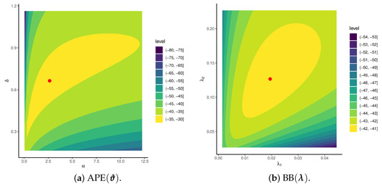
Figure 2. Contours of APE and BB model parameters from P-FFC-BB data.

3.2. Interval Estimation

To acquire the $(1-\upsilon )100\%$ ACI estimators for the APE parameters $\alpha$, $\delta$, $R\left(x\right)$, and $h\left(x\right)$, as well as for the BB parameters ${\lambda }_i$$(i=1,2)$, we utilize the asymptotic properties of their MLEs based on large-sample theory. Under standard regularity conditions, the joint asymptotic distribution of $\widehat{\mathsf{\Lambda }}$ is bivariate normal with mean vector $\mathsf{\Lambda }$ and variance–covariance (VC) matrix ${\Im }_1^{-1}(·)$, where ${\Im }_1(·)$ denotes the Fisher information (FI) matrix. However, due to the complex structure of the second-order partial derivatives of the log-likelihood function ${\mathbb{L}}_1^{\circ }(·)$, obtaining a closed-form expression for the FI matrix ${\Im }_1(·)$ is generally infeasible. Consequently, the observed information matrix evaluated at $\widehat{\mathsf{\Lambda }}$ is used to approximate ${\Im }_1^{-1}(·)$ as

$$\begin{array}{c}{\widehat{\Im }}_1^{-1}\left(\widehat{\mathsf{\Lambda }}\right)=\left[\begin{array}{cc}-l_{11}& -l_{12}\\ -l_{21}& -l_{22}\end{array}\right]={\left[\begin{array}{cc}{\widehat{{\rm Y}}}_{11}& {\widehat{{\rm Y}}}_{12}\\ {\widehat{{\rm Y}}}_{21}& {\widehat{{\rm Y}}}_{22}\end{array}\right]}_{(\widehat{\mathsf{\Lambda }}=\mathsf{\Lambda })},\hfill \end{array}$$

(19)

with the items, $l_{ij},i,j=1,2$, expressed and reported in Appendix A.

Constructing the $(1-\upsilon )100\%$ ACIs for $R\left(x\right)$ and $h\left(x\right)$ requires estimates of the variances of $\widehat{R}\left(x\right)$ and $\widehat{h}\left(x\right)$. A commonly employed approach for this purpose is the delta method, which provides a convenient way to approximate the variance of functions of estimated parameters. For an in-depth discussion of the delta method, refer to Greene [18]. Using this technique, the approximate variances of the estimators for $R\left(x\right)$ and $h\left(x\right)$ are obtained as

$${\widehat{{\rm Y}}}_{33}\approx {\left[{\Sigma }_R{\widehat{\Im }}_1^{-1}\left(\mathit{\vartheta }\right){\Sigma }_R^{\top }\right]}_{(\widehat{\mathsf{\Lambda }}=\mathsf{\Lambda })}\mathrm{and}{\widehat{{\rm Y}}}_{44}\approx {\left[{\Sigma }_h{\widehat{\Im }}_1^{-1}\left(\mathsf{\Lambda }\right){\Sigma }_h^{\top }\right]}_{(\widehat{\mathsf{\Lambda }}=\mathsf{\Lambda })}.$$

(20)

We first obtain ${\Sigma }_R=\left({\displaystyle \frac{\partial R}{\partial \alpha }}{\displaystyle \frac{\partial R}{\partial \delta }}\right){|}_{(\widehat{\mathsf{\Lambda }}=\mathsf{\Lambda })}$ and ${\Sigma }_h=\left({\displaystyle \frac{\partial h}{\partial \alpha }}{\displaystyle \frac{\partial h}{\partial \delta }}\right){|}_{(\widehat{\mathsf{\Lambda }}=\mathsf{\Lambda })}$, where

$${\displaystyle \begin{array}{c}{\displaystyle \frac{\partial R}{\partial \alpha }}={\displaystyle \frac{1}{\alpha -1}}\left[e^{-\delta x}{\alpha }^{-e^{-\delta x}}+({\alpha }^{-e^{-\delta x}}-1){(\alpha -1)}^{-1}\right],\hfill \\ {\displaystyle \frac{\partial R}{\partial \delta }}={\displaystyle \frac{\alpha \log \left(\alpha \right)x{e}^{-\delta x}{\alpha }^{-e^{-\delta x}}}{\alpha -1}},\hfill \\ {\displaystyle \frac{\partial h}{\partial \alpha }}=\delta \left[{\displaystyle \frac{\left[1-\log \left(\alpha \right)e^{-\delta x}\right]{\alpha }^{-e^{-\delta x}}-1}{\alpha e^{\delta x}{({\alpha }^{-e^{-\delta x}}-1)}^2}}\right],\hfill \end{array}}$$

and

$${\displaystyle \begin{array}{c}{\displaystyle \frac{\partial h}{\partial \delta }}=\log \left(\alpha \right)\left[{\displaystyle \frac{\left[1+\delta x\left(\log \left(\alpha \right)e^{-\delta x}-1\right)\right]{\alpha }^{-e^{-\delta x}}+\delta x-1}{e^{\delta x}{({\alpha }^{-e^{-\delta x}}-1)}^2}}\right].\hfill \end{array}}$$

On the other hand, by replacing $\mathit{\lambda }$ with their $\widehat{\mathit{\lambda }}$, the approximated VC matrix of the BB parameters $\mathit{\lambda }$ (symbolized by ${\widehat{\Im }}_2^{-1}(·)$) is given by

$$\begin{array}{c}{\widehat{\Im }}_2^{-1}\left(\widehat{\mathit{\lambda }}\right)={\left[\begin{array}{cc}-l_{33}& -l_{34}\\ -l_{43}& -l_{44}\end{array}\right]}_{(\widehat{\mathit{\lambda }}=\mathit{\lambda })}^{-1},\hfill \end{array}$$

(21)

with the items, $l_{ij},i,j=3,4$, expressed and reported in Appendix B.

It is evident from the VC matrices in (19) and (21) that the likelihood equations for APE$\left(\mathsf{\Lambda }\right)$ and BB$\left(\mathit{\lambda }\right)$ cannot be expressed in closed form. Therefore, again, we recommend using the NR iterative procedure to compute ${{\rm Y}}_{ij},i,j=1,2,3,4$. Hence, at a significance percentage $\upsilon 100\%$, the $100(1-\upsilon )100\%$ two-sided ACI limits of $\alpha$, $\delta$, $R\left(x\right)$, $h\left(x\right)$, or ${\lambda }_i,$$i=1,2$ (say, ℧ for brevity) are

$${\widehat{\mho }}_i\pm z_{\frac{\upsilon }{2}}\sqrt{{\widehat{{\rm Y}}}_{ii}},$$

(22)

where ${\widehat{{\rm Y}}}_{ii},i=1,2,\dots ,6,$ represent the approximated variances of $\alpha$, $\delta$, $R\left(x\right)$, $h\left(x\right)$, and ${\lambda }_i,i=1,2$, given by (19) and (20), and $z_{{\displaystyle \frac{\upsilon }{2}}}$ is the upper ${\displaystyle \frac{\upsilon }{2}}$th percentile point of the standard Gaussian distribution.

4. Bayesian Inference

The Bayesian framework allows prior beliefs or expert knowledge to be incorporated into the inference process for unknown parameters. In this setting, the parameters $\alpha$ and $\delta$ of the APE lifetime distribution are treated as random variables, with their prior distributions representing any available prior information. A particularly convenient and flexible choice is the gamma conjugate prior, as highlighted by Kundu [19] and Dey et al. [20]. The gamma distribution provides substantial modeling versatility, making it suitable for encoding a broad range of subjective or empirical prior beliefs. Independent gamma priors are assigned to $(\alpha ,\delta )$ and $({\lambda }_1,{\lambda }_2)$ to ensure positive support and conjugacy, offering flexibility in specifying both weakly and moderately informative beliefs. Here, we assume that $\alpha$ and $\delta$ follow independent gamma priors, specified as $\alpha \sim \mathrm{Gamma}(a_1,b_1)$ and $\delta \sim \mathrm{Gamma}(a_2,b_2)$, where $a_i,b_i>0$ for $i=1,2$. These hyperparameters are selected to reflect prior information relevant to the $\mathrm{APE}\left(\mathit{\lambda }\right)$ distribution parameters. Under this independence assumption, the joint prior PDF of $\alpha$ and $\delta$, denoted by ${\omega }_1(·)$, takes the form

$${\omega }_1\left(\mathit{\lambda }\right)\propto {\alpha }^{a_1-1}{\delta }^{a_2-1}{e}^{-\left(b_1\alpha +b_2\delta \right)},\alpha ,\delta >0,$$

(23)

where $a_i$ and $b_i$$(i=1,2)$ are assumed to be known. By substituting (12) and (23) into the Bayes’ theorem, the joint posterior PDF of APE$\left(\mathit{\vartheta }\right)$, denoted by ${\Phi }_1(·)$, can be expressed as

$${\Phi }_1\left(\mathsf{\Lambda }\right|\mathbf{r},\mathbf{y})\propto {\displaystyle \frac{{\alpha }^{n+a_1-1}{\left(\log \left(\alpha \right)\right)}^k}{{\left(\alpha -1\right)}^n}}{\delta }^{k+a_2-1}{e}^{-\delta \left(b_2+k\overline{y}\right)}{e}^{-b_1\alpha -\log \left(\alpha \right){\sum }_{i=1}^k{e}^{-\delta y_i}}\prod _{i=1}^k{\left(1-{\alpha }^{-e^{-\delta y_i}}\right)}^{m_i^{*}},$$

(24)

where its normalized term, say $\Xi$, is given by

$$\begin{array}{c}{\Xi }_1={\int }_{\alpha }{\int }_{\delta }{\mathcal{L}}_{\varsigma }\left(\mathit{\lambda }\right|\mathbf{y})\times p\left(\mathit{\lambda }\right)\mathrm{d}\alpha \mathrm{d}\delta .\hfill \end{array}$$

Similarly, for the BB$\left(\mathit{\lambda }\right)$ parameters, we assume that they are mutually independent and that each follows a gamma prior distribution, denoted by $G_{{\lambda }_1}(a_3,b_3)$ and $G_{{\lambda }_2}(a_4,b_4)$, respectively. The hyperparameters $a_i>0$ and $b_i>0$ for $i=3,4$ are assumed to be known. Under this independence assumption, the joint gamma PDF of ${\lambda }_i$$(i=1,2)$, denoted by ${\omega }_2(·)$, is given by

$${\omega }_2\left(\mathit{\lambda }\right)\propto {\lambda }_1^{{\alpha }_3-1}{\lambda }_2^{{\alpha }_4-1}{e}^{-({\beta }_3{\lambda }_1+{\beta }_4{\lambda }_2)},{\lambda }_i>0,i=1,2.$$

(25)

From (16) and (25), the joint posterior PDF of BB$\left(\mathit{\lambda }\right)$ (say, ${\Phi }_2(·)$) can be expressed as

$${\Phi }_2\left(\left.\mathbf{R}=\mathbf{r}\right|\mathit{\lambda }\right)={\Xi }_2^{-1}{\displaystyle \frac{{\lambda }_1^{{\alpha }_3-1}{\lambda }_2^{{\alpha }_4-1}{e}^{-({\beta }_3{\lambda }_1+{\beta }_4{\lambda }_2)}}{{\left(B\left({\lambda }_1,{\lambda }_2\right)\right)}^{k-1}}}\prod _{i=1}^{k-1}B\left({\lambda }_1+r_i,{\lambda }_2+n^{*}\right),$$

(26)

where ${\Xi }_2={\int }_0^{\infty }{\int }_0^{\infty }{\mathcal{L}}_2\left(\left.\mathbf{R}=\mathbf{r}\right|\mathit{\lambda }\right)\times {{\rm Y}}_2\left(\mathit{\lambda }\right)\mathrm{d}{\lambda }_1\mathrm{d}{\lambda }_2$.

The squared error loss (SEL) is a commonly used symmetric loss function for Bayesian estimation. Under this criterion, the Bayes estimator, denoted by ${\tilde{\pi }}_S$, corresponds to the posterior mean based on the observed data. Formally, the SEL function (written as ${\zeta }_S$) and the resulting Bayes estimator ${\tilde{\pi }}_S$ can be defined as

$${\eta }_S(\pi ,{\tilde{\pi }}_S)={\left({\tilde{\pi }}_S-\pi \right)}^2,$$

and

$${\tilde{\pi }}_S=\mathbb{E}\left[\pi \mid \mathrm{data}\right]={\Xi }_i^{-1}{\int }_{\pi }\pi {\Phi }_i(\pi \mid \mathrm{data})\mathrm{d}\pi ,i=1,2,$$

(27)

respectively; see Martz and Waller [21].

In contrast to the symmetric SEL, the generalized entropy loss (GEL) introduces an asymmetric estimation criterion. This loss function is particularly suitable when the consequences of overestimation and underestimation are not equally severe. The GEL, denoted by ${\zeta }_G$, is defined as

$${\eta }_G(\pi ,{\tilde{\pi }}_G)\propto {\left({\displaystyle \frac{{\tilde{\pi }}_G}{\pi }}\right)}^{\tau }-\tau \log \left({\displaystyle \frac{{\tilde{\pi }}_G}{\pi }}\right)-1,\tau \ne 0,$$

(28)

where ${\tilde{\pi }}_G$ denotes the derived Bayes estimator from GEL.

As seen from (28), the generalized entropy loss is minimized when ${\tilde{\pi }}_G=\pi$. Notably, by setting $\tau =-1$ in (28), the asymmetric Bayes estimator ${\tilde{\pi }}_G$ reduces to the symmetric Bayes estimator ${\tilde{\pi }}_S$. When $\tau >0$, the GE loss penalizes overestimation more heavily than underestimation, whereas for $\tau <0$, the opposite effect occurs. Based on (28), the Bayes estimator ${\tilde{\pi }}_G$ of $\pi$ is given by

$${\tilde{\pi }}_G={\left[\mathbb{E}\left({\pi }^{-\tau }\mid \mathrm{data}\right)\right]}^{-{\displaystyle \frac{1}{\tau }}}.$$

For more details, see Dey et al. [22]. Due to the nonlinear form of the posterior distribution, ${\Phi }_1(·)$, presented in (24), closed-form expressions for the Bayes estimators of $\mathsf{\Lambda }$, $R\left(x\right)$, or $h\left(x\right)$ against both SEL and GEL functions are analytically intractable.

It is worth mentioning that the SEL function is a natural default choice due to its symmetry and simplicity, yielding posterior means as Bayes estimators. In contrast, the GEL function introduces asymmetry to accommodate scenarios where overestimation and underestimation incur unequal costs.

Consequently, we utilize the MCMC technique to approximate the Bayes estimators ${\tilde{\pi }}_S$ and ${\tilde{\pi }}_G$ and to construct the associated BCI estimators. To generate such samples, it is first necessary to derive the full-conditional posterior PDFs of $\alpha$ and $\delta$, as follows:

$${\Phi }_1^{\alpha }\left(\alpha \right|\delta ,\mathbf{r},\mathbf{y})\propto {\displaystyle \frac{{\alpha }^{n+a_1-1}{\left(\log \left(\alpha \right)\right)}^k}{{\left(\alpha -1\right)}^n}}{e}^{-b_1\alpha -\log \left(\alpha \right){\sum }_{i=1}^k{e}^{-\delta y_i}}\prod _{i=1}^k{\left(1-{\alpha }^{-e^{-\delta y_i}}\right)}^{m_i^{*}},$$

(29)

and

$${\Phi }_1^{\delta }\left(\delta \right|\alpha ,\mathbf{r},\mathbf{y})\propto {\delta }^{k+a_2-1}{e}^{-\left(\delta \left(b_2+k\overline{y}\right)+\log \left(\alpha \right){\sum }_{i=1}^k{e}^{-\delta y_i}\right)}\prod _{i=1}^k{\left(1-{\alpha }^{-e^{-\delta y_i}}\right)}^{m_i^{*}},$$

(30)

respectively.

From (29) and (30), it is clear that the full conditional PDFs of $\alpha$ and $\delta$ do not belong to any standard family of statistical distributions. Therefore, direct sampling from the conditional densities ${\Phi }_1^{\alpha }(·)$ and ${\Phi }_1^{\delta }(·)$ using conventional sampling methods is not possible. To handle this difficulty, as shown in Figure 3, we employ the Metropolis–Hastings (MH) algorithm with normally distributed proposal densities to generate posterior samples. This allows us to obtain Bayesian point estimates and credible intervals for the APE model parameters $\alpha$, $\delta$, $R\left(x\right)$, and $h\left(x\right)$; see Algorithm 1.

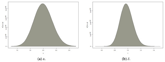
Figure 3. The posterior PDFs of $\alpha$ and $\delta$ from APE (2, 1) and BB (1, 1).

On the other hand, from (26), the full-conditional PDFs of the BB parameters ${\lambda }_i,$$i=1,2$, can be formulated as

$${\Phi }_2^{{\lambda }_1}\left({\lambda }_1\right|{\lambda }_2,\left.\mathbf{R}=\mathbf{r}\right)\propto {\displaystyle \frac{{\lambda }_1^{{\alpha }_3-1}{e}^{-{\beta }_3{\lambda }_1}}{{\left(B\left({\lambda }_1,{\lambda }_2\right)\right)}^{k-1}}}\prod _{i=1}^{k-1}B\left({\lambda }_1+r_i,{\lambda }_2+n^{*}\right),$$

(31)

and

$${\Phi }_2^{{\lambda }_2}\left({\lambda }_2\right|{\lambda }_1,\left.\mathbf{R}=\mathbf{r}\right)\propto {\displaystyle \frac{{\lambda }_2^{{\alpha }_4-1}{e}^{-{\beta }_4{\lambda }_2}}{{\left(B\left({\lambda }_1,{\lambda }_2\right)\right)}^{k-1}}}\prod _{i=1}^{k-1}B\left({\lambda }_1+r_i,{\lambda }_2+n^{*}\right),$$

(32)

respectively.

As expected from (31) and (32), the conditional PDFs of ${\lambda }_i$$(i=1,2)$ do not correspond to any standard statistical distribution. Consequently, direct sampling from these posteriors using conventional methods is not feasible. To overcome this, again, we employ the MH algorithm, following the same procedure described in Algorithm 1, to generate MCMC samples for ${\lambda }_i$$(i=1,2)$.

Algorithm 1 The MCMC (MH-based) Generation Steps

1: Input: Start with $\varsigma =1$  2: Input: Assign starting points of $\alpha$ as $\widehat{\alpha }$ and of $\delta$ as $\widehat{\delta }$  3: Output: Get ${\alpha }^{★}$ from $N(\widehat{\alpha },{\widehat{{\rm Y}}}_{11})$  4: Output: Calculate ${\ell }_{\alpha }=\min \left[1,\frac{{\mathsf{\Phi }}_1^{\alpha }\left({\alpha }^{★}\right|{\delta }^{(\varsigma -1)},\mathbf{r},\mathbf{y})}{{\Phi }_1^{\alpha }\left({\alpha }^{(\varsigma -1)}\right|{\delta }^{(\varsigma -1)},\mathbf{r},\mathbf{y})}\right]$  5: Output: Get an uniform variate (say, u) from $U(0,1)$  6: Output: Store ${\alpha }^{★}$  7: As ${\alpha }^{\left(\varsigma \right)} u\le {\ell }_{\alpha }$  8: Else set ${\alpha }^{(\varsigma -1)}$  9: Input: Redo Steps 3–10 for ${\delta }^{\left(\varsigma \right)}$ from ${\Phi }_1^{\delta }\left(\delta \right|\alpha ,\mathbf{r},\mathbf{y})$ 10: Output: Obtain $R^{\left(\varsigma \right)}$ from (3) and $h^{\left(\varsigma \right)}$ from (4) 11: Input: Set $\varsigma =\varsigma +1$ 12: Input: Redo Steps 1–13 $\mathbb{W}$ times, and remove ${\mathbb{W}}^{•}$ as a burn-in size 13: Output: Compute $$\begin{array}{cc}\tilde{\alpha }\hfill & ={\displaystyle \frac{1}{{\mathbb{W}}^{★★}}}{\sum }_{\varsigma ={\mathbb{W}}^{•}+1}^{\mathbb{W}}{\alpha }^{\left(\varsigma \right)},\hfill \\ \tilde{\delta }& ={\displaystyle \frac{1}{{\mathbb{W}}^{★★}}}{\sum }_{\varsigma ={\mathbb{W}}^{•}+1}^{\mathbb{W}}{\delta }^{\left(\varsigma \right)},\hfill \\ \tilde{R}\left(x\right)& ={\displaystyle \frac{1}{{\mathbb{W}}^{★★}}}{\sum }_{\varsigma ={\mathbb{W}}^{•}+1}^{\mathbb{W}}{R}^{\left(\varsigma \right)}\left(x\right),\hfill \end{array}$$ and $$\begin{array}{cc}\tilde{h}\left(x\right)\hfill & ={\displaystyle \frac{1}{{\mathbb{W}}^{★★}}}{\sum }_{\varsigma ={\mathbb{W}}^{•}+1}^{\mathbb{W}}{h}^{\left(\varsigma \right)}\left(x\right),\hfill \end{array}$$ where ${\mathbb{W}}^{★★}=\mathbb{W}-{\mathbb{W}}^{•}$ 14: Input: Sort ${\alpha }^{\left(\varsigma \right)}$, ${\delta }^{\left(\varsigma \right)}$, $R^{\left(\varsigma \right)}\left(x\right)$, and $h^{\left(\varsigma \right)}\left(x\right)$ (for $\varsigma ={\mathbb{W}}^{•}+1,{\mathbb{W}}^{•}+2,\dots ,\mathbb{W}$) 15: Output: Compute the $100(1-\varrho )\%$ BCI estimators of $\alpha$, $\delta$, $R\left(x\right)$, and $h\left(x\right)$ as $$\begin{array}{c}\left\{{\alpha }^{\left[\left({\displaystyle \frac{\upsilon }{2}}\right){\mathbb{W}}^{★★}\right]},{\alpha }^{\left[\left(1-{\displaystyle \frac{\upsilon }{2}}\right){\mathbb{W}}^{★★}\right]}\right\},\hfill \\ \left\{{\delta }^{\left[\left({\displaystyle \frac{\upsilon }{2}}\right){\mathbb{W}}^{★★}\right]},{\delta }^{\left[\left(1-{\displaystyle \frac{\upsilon }{2}}\right){\mathbb{W}}^{★★}\right]}\right\},\hfill \\ \left\{R^{\left[\left({\displaystyle \frac{\upsilon }{2}}\right){\mathbb{W}}^{★★}\right]}\left(x\right),R^{\left[\left(1-{\displaystyle \frac{\upsilon }{2}}\right){\mathbb{W}}^{★★}\right]}\left(x\right)\right\},\hfill \end{array}$$ and $$\begin{array}{c}\left\{h^{\left[\left({\displaystyle \frac{\upsilon }{2}}\right){\mathbb{W}}^{★★}\right]}\left(x\right),h^{\left[\left(1-{\displaystyle \frac{\upsilon }{2}}\right){\mathbb{W}}^{★★}\right]}\left(x\right)\right\}\hfill \end{array}$$

5. Monte Carlo Comparisons

This section presents a detailed evaluation of the proposed theoretical results, focusing on point and interval estimation for the APE $(\alpha ,\delta )$ parameters. It also considers related reliability measures, including the RF $R\left(x\right)$ and FRF $h\left(x\right)$.

5.1. Simulation Setups

A Monte Carlo simulation is conducted based on samples generated from two populations of APE$\left(\mathit{\vartheta }\right)$, namely Pop-A:(0.8, 0.5) and Pop-B:(2, 1). To achieve this, the proposed P-FFC-BB strategy is replicated 2000 times. To generate data from the APE lifetime model under the proposed censoring plan, we follow the steps outlined in Algorithm 2. At $x=0.1$, the true values of $R\left(x\right)$ and $h\left(x\right)$ are approximately 0.94588 and 0.55494 from Pop-A and approximately 0.93181 and 0.71897 from Pop-B, respectively, serving as reference values for assessing estimation accuracy. The performance of the estimators for $\alpha$, $\delta$, $R\left(x\right)$, and $h\left(x\right)$ is investigated under varying experimental settings by changing ${\lambda }_i,i=1,2$ (BB coefficients), $m(=2,5)$ (group size), $n(30,60,80)$ (total number of test units), and different choices of k (number of failed units). According to the mechanism of the proposed censoring, the life test ends when the observed number of failures k is reached for each given n.

Following the MCMC strategy described in Section 4, the simulation uses $\mathbb{W}=12,000$ iterations, discarding the first ${\mathbb{W}}^{•}=2000$ as burn-in. Posterior estimates, along with their 95% BCI/HPD interval estimates, are obtained for $\alpha$, $\delta$, $R\left(x\right)$, and $h\left(x\right)$. For further analysis, after collecting 2000 P-FFC-BB samples, we employ two packages within the R software version 4.2.2 environment:

• A ‘maxLik’ (by Henningsen and Toomet [23]) for maximum likelihood calculations;
• A ‘coda’ (by Plummer et al. [24]) for simulating and analyzing posterior samples.

It should be noted here that the MLEs $\widehat{\alpha }$ and $\widehat{\delta }$ (obtained by solving the score Equations (14) and (15)) and the MLEs ${\widehat{\lambda }}_i,i=1,2$ (obtained by solving the score Equations (18) and (17)) are computed using the NR iterative algorithm using ‘maxLik’. Computations are performed in R, and convergence is declared when the absolute change in the log-likelihood between successive iterations is less than ${10}^{-6}$.

To further evaluate the sensitivity of the estimation procedures with respect to the BB removal mechanism, we examine two parameter configurations of the BB$({\lambda }_1,{\lambda }_2)$ distribution, namely BB-1:(0.5, 0.5) and BB-2:(1.5, 1.5). One of the key challenges in Bayesian inference is the appropriate specification of hyperparameters. In this study, we follow the prior elicitation approach outlined by Kundu [19] to determine the values of the hyperparameters ${\alpha }_i$ and ${\beta }_i$$(i=1,2)$ in the joint gamma prior distribution. Accordingly, two prior settings are considered:

• For Pop-A:(0.8, 0.5):

  –

  Prior-A:[PA] $(a_1,a_2)=(4,2.5)$ with $b_i=5$ for $i=1,2$;

  –

  Prior-B:[PB] $(a_1,b_2)=(8,5)$ with $b_i=10$ for $i=1,2$.

• For Pop-B:(2, 1):

  –

  Prior-A:[PA] $(a_1,a_2)=(10,5)$ with $b_i=5$ for $i=1,2$;

  –

  Prior-B:[PB] $(a_1,b_2)=(20,10)$ with $b_i=10$ for $i=1,2$.

The corresponding hyperparameters for each unknown parameter are determined using the method of moments, based on simulated censoring proportions. Two prior settings are considered—PA (weakly informative) and PB (more informative)—to evaluate sensitivity and robustness. This strategy ensures that posterior inference remains primarily data-driven while offering additional stability in scenarios involving small sample sizes or heavy censoring.

Algorithm 2 P-FFC-BB generation procedure

1: Input: Set the APE$\left(\mathit{\vartheta }\right)$ population parameters  2: Input: Specify the BB$({\lambda }_1,{\lambda }_2)$ distribution parameters  3: Input: Assign values for m, n, and k  4: Output: Generate $r_1\sim BB\left(n^{★}-k,{\lambda }_1,{\lambda }_2\right)$  5: Output: For $i=2,3,\dots ,k-1$, generate $r_i\sim BB\left(n^{★}-k-{\sum }_{j=1}^{i-1}{r}_j,{\lambda }_1,{\lambda }_2\right)$  6: Output: Determine $r_k$ as $$r_k=\left\{\begin{array}{cc}{n}^{★}-k-{\displaystyle \sum _{i=1}^{k-1}}{r}_i,\hfill & \mathrm{if}\left(n^{★}-k-{\displaystyle \sum _{i=1}^{k-1}}{r}_i\right)>0,\hfill \\ 0,\hfill & \mathrm{otherwise}\hfill \end{array}\right.$$  7: Output: Generate $D_i\sim U(0,1)$ for $i=1,2,\dots ,k$  8: Output: Compute $$T_i=D_i^{{\left(i+\sum _{j=k-i+1}^k{r}_j\right)}^{-1}},i=1,2,\dots ,k$$  9: Output: Compute $$U_i=T_k{T}_{k-1}\dots T_{k-i+1},i=1,2,\dots ,k$$ 10: Output: Obtain $$U_i^{★}=1-U_i,i=1,2,\dots ,k$$ 11: Output: Stop and collect $$y_i=F^{-1}(u_i^{★};\alpha ,\delta ),i=1,2,\dots ,k$$

We now evaluate the introduced estimators obtained for the parameters $\alpha$, $\delta$, $R\left(x\right)$, and $h\left(x\right)$ (say, $\varrho$ for short) using the following performance criteria:

• Root Mean Squared Error (RMSE):

  $$\mathrm{RMSE}\left(\ddot{\varrho }\right)=\sqrt{{\displaystyle \frac{1}{2000}}\sum _{i=1}^{2000}{\left({\ddot{\varrho }}^{\left[i\right]}-\varrho \right)}^2}.$$
• Average Relative Absolute Bias (ARAB):

  $$\mathrm{ARAB}\left(\ddot{\varrho }\right)={\displaystyle \frac{1}{2000}}\sum _{i=1}^{2000}{\ddot{\varrho }}^{-1}\left|{\ddot{\varrho }}^{\left[i\right]}-\varrho \right|.$$
• Average Interval Length (AIL):

  $${\mathrm{AIL}}_{95\%}\left(\varrho \right)={\displaystyle \frac{1}{2000}}\sum _{i=1}^{2000}\left({\mathcal{U}}_{{\ddot{\varrho }}^{\left[i\right]}}-{\mathcal{L}}_{{\ddot{\varrho }}^{\left[i\right]}}\right),$$

  where ${\mathcal{L}}_{{\ddot{\varrho }}^{\left[i\right]}}$ and ${\mathcal{U}}_{{\ddot{\varrho }}^{\left[i\right]}}$ denote the (lower and upper) 95% interval bounds.
• Coverage Percentage (CP):

  $${\mathrm{CP}}_{95\%}\left(\varrho \right)={\displaystyle \frac{1}{2000}}\sum _{i=1}^{2000}{\mathbb{D}}_{\left({\mathcal{L}}_{{\ddot{\varrho }}^{\left[i\right]}},{\mathcal{U}}_{{\ddot{\varrho }}^{\left[i\right]}}\right)}\left(\varrho \right),$$

  where $\mathbb{D}(·)$ is the indicator function, taking the value 1 if $\varrho$ lies within the interval $\left[{\mathcal{L}}_{{\ddot{\varrho }}^{\left[i\right]}},{\mathcal{U}}_{{\ddot{\varrho }}^{\left[i\right]}}\right]$; otherwise, it is 0.

5.2. Simulation Results and Interpretation

From Table 1, Table 2, Table 3, Table 4, Table 5, Table 6, Table 7 and Table 8, for BB-1, we focus on estimation methods yielding the lowest RMSE, ARAB, and AIL values while maintaining the highest CP values. For brevity, the remaining simulation results based on BB-2 are provided in the Supplementary File. The main findings can be summarized as follows:

Table 1. The RMSE (1st Col.) and ARAB (2nd Col.) results of $\alpha$ from BB-1.

$({\mathit{\lambda }}_1,{\mathit{\lambda }}_2)$	m	$(\mathit{n},\mathit{k})$	MLE		SEL				GEL ($\mathit{\tau }=-2$)				GEL ($\mathit{\tau }=+2$)
					PA		PB		PA		PB		PA		PB
Pop-1
(0.5, 0.5)	2	(30, 10)	1.043	0.843	0.205	0.245	0.196	0.242	0.154	0.189	0.187	0.233	0.145	0.181	0.151	0.183
		(30, 20)	0.645	0.343	0.082	0.099	0.079	0.097	0.054	0.050	0.077	0.097	0.037	0.046	0.037	0.047
		(60, 20)	0.931	0.884	0.124	0.138	0.111	0.136	0.056	0.065	0.103	0.128	0.051	0.064	0.052	0.065
		(60, 40)	0.562	0.306	0.054	0.058	0.046	0.049	0.035	0.044	0.036	0.045	0.031	0.038	0.033	0.041
		(80, 30)	0.915	0.348	0.119	0.134	0.108	0.132	0.056	0.063	0.101	0.126	0.050	0.062	0.051	0.063
		(80, 60)	0.526	0.301	0.045	0.046	0.041	0.043	0.034	0.041	0.035	0.042	0.026	0.033	0.027	0.034
	5	(30, 10)	0.359	0.226	0.043	0.046	0.041	0.041	0.033	0.040	0.033	0.041	0.025	0.032	0.026	0.033
		(30, 20)	0.297	0.199	0.039	0.042	0.028	0.035	0.027	0.030	0.028	0.034	0.013	0.016	0.013	0.017
		(60, 20)	0.347	0.212	0.042	0.046	0.033	0.041	0.031	0.034	0.032	0.039	0.020	0.025	0.025	0.031
		(60, 40)	0.157	0.122	0.034	0.038	0.022	0.022	0.012	0.014	0.012	0.015	0.009	0.011	0.011	0.014
		(80, 30)	0.346	0.203	0.039	0.044	0.032	0.038	0.028	0.034	0.031	0.035	0.019	0.023	0.020	0.025
		(80, 60)	0.144	0.115	0.028	0.029	0.021	0.021	0.007	0.009	0.009	0.010	0.002	0.002	0.002	0.002
Pop-2
(0.5, 0.5)	2	(30, 10)	1.234	0.584	0.219	0.263	0.211	0.261	0.145	0.178	0.202	0.252	0.148	0.183	0.154	0.187
		(30, 20)	0.824	0.516	0.071	0.084	0.067	0.082	0.062	0.073	0.065	0.081	0.057	0.072	0.058	0.073
		(60, 20)	1.199	0.568	0.135	0.156	0.126	0.154	0.072	0.084	0.119	0.149	0.066	0.082	0.068	0.084
		(60, 40)	0.765	0.484	0.069	0.078	0.063	0.077	0.061	0.071	0.061	0.076	0.055	0.069	0.057	0.070
		(80, 30)	0.896	0.522	0.124	0.138	0.111	0.136	0.067	0.079	0.103	0.128	0.062	0.078	0.063	0.079
		(80, 60)	0.562	0.347	0.060	0.067	0.054	0.067	0.053	0.062	0.054	0.066	0.049	0.061	0.050	0.062
	5	(30, 10)	0.522	0.327	0.058	0.066	0.047	0.058	0.043	0.052	0.047	0.053	0.037	0.046	0.038	0.047
		(30, 20)	0.473	0.306	0.045	0.046	0.030	0.035	0.027	0.032	0.028	0.033	0.005	0.006	0.010	0.012
		(60, 20)	0.515	0.323	0.056	0.064	0.043	0.050	0.039	0.047	0.040	0.048	0.020	0.025	0.023	0.028
		(60, 40)	0.240	0.184	0.035	0.037	0.027	0.027	0.007	0.009	0.008	0.010	0.005	0.005	0.007	0.008
		(80, 30)	0.496	0.309	0.046	0.050	0.039	0.038	0.028	0.035	0.031	0.037	0.019	0.024	0.020	0.025
		(80, 60)	0.222	0.174	0.022	0.022	0.019	0.019	0.007	0.007	0.007	0.008	0.002	0.002	0.003	0.004

Table 2. The RMSE (1st Col.) and ARAB (2nd Col.) results of $\delta$ from BB-1.

$({\mathit{\lambda }}_1,{\mathit{\lambda }}_2)$	m	$(\mathit{n},\mathit{k})$	MLE		SEL				GEL ($\mathit{\tau }=-2$)				GEL ($\mathit{\tau }=+2$)
					PA		PB		PA		PB		PA		PB
Pop-1
(0.5, 0.5)	2	(30, 10)	0.330	0.504	0.245	0.490	0.239	0.460	0.227	0.453	0.224	0.447	0.217	0.413	0.202	0.403
		(30, 20)	0.254	0.470	0.205	0.409	0.202	0.394	0.194	0.388	0.186	0.371	0.183	0.352	0.173	0.345
		(60, 20)	0.325	0.498	0.238	0.475	0.230	0.441	0.220	0.440	0.214	0.427	0.214	0.411	0.198	0.395
		(60, 40)	0.247	0.442	0.173	0.346	0.172	0.324	0.158	0.315	0.157	0.313	0.155	0.285	0.139	0.277
		(80, 30)	0.253	0.467	0.201	0.402	0.198	0.383	0.188	0.375	0.174	0.348	0.170	0.305	0.145	0.288
		(80, 60)	0.247	0.441	0.119	0.231	0.116	0.210	0.098	0.189	0.095	0.189	0.095	0.177	0.087	0.173
	5	(30, 10)	0.247	0.442	0.156	0.311	0.152	0.271	0.137	0.260	0.137	0.230	0.115	0.213	0.101	0.201
		(30, 20)	0.246	0.437	0.089	0.174	0.087	0.170	0.084	0.166	0.082	0.160	0.080	0.156	0.078	0.155
		(60, 20)	0.246	0.439	0.117	0.223	0.112	0.183	0.096	0.181	0.091	0.170	0.084	0.168	0.079	0.158
		(60, 40)	0.245	0.430	0.053	0.092	0.043	0.086	0.033	0.065	0.030	0.048	0.010	0.020	0.008	0.015
		(80, 30)	0.246	0.436	0.081	0.137	0.070	0.116	0.063	0.100	0.051	0.092	0.046	0.092	0.046	0.090
		(80, 60)	0.242	0.424	0.050	0.089	0.028	0.056	0.026	0.044	0.021	0.041	0.003	0.006	0.003	0.005
Pop-2
(0.5, 0.5)	2	(30, 10)	0.539	0.440	0.299	0.298	0.294	0.271	0.263	0.262	0.227	0.223	0.223	0.211	0.208	0.207
		(30, 20)	0.465	0.431	0.232	0.229	0.230	0.219	0.215	0.215	0.184	0.180	0.180	0.175	0.174	0.173
		(60, 20)	0.533	0.439	0.267	0.266	0.267	0.248	0.243	0.242	0.188	0.185	0.185	0.178	0.176	0.176
		(60, 40)	0.461	0.428	0.173	0.167	0.167	0.154	0.151	0.150	0.138	0.133	0.133	0.129	0.128	0.128
		(80, 30)	0.462	0.428	0.177	0.168	0.169	0.161	0.159	0.159	0.156	0.144	0.145	0.134	0.130	0.130
		(80, 60)	0.457	0.414	0.075	0.059	0.075	0.059	0.059	0.057	0.057	0.056	0.054	0.053	0.051	0.050
	5	(30, 10)	0.460	0.422	0.138	0.128	0.128	0.122	0.120	0.119	0.119	0.101	0.102	0.092	0.088	0.087
		(30, 20)	0.457	0.401	0.063	0.049	0.053	0.049	0.051	0.046	0.043	0.043	0.042	0.041	0.041	0.041
		(60, 20)	0.457	0.411	0.069	0.058	0.065	0.053	0.053	0.053	0.053	0.051	0.049	0.048	0.046	0.045
		(60, 40)	0.448	0.394	0.047	0.042	0.032	0.028	0.028	0.027	0.024	0.024	0.022	0.022	0.021	0.021
		(80, 30)	0.456	0.401	0.051	0.044	0.042	0.042	0.041	0.041	0.033	0.028	0.022	0.022	0.021	0.021
		(80, 60)	0.448	0.392	0.028	0.023	0.026	0.021	0.018	0.017	0.017	0.017	0.015	0.015	0.014	0.014

Table 3. The RMSE (1st Col.) and ARAB (2nd Col.) results of $R\left(x\right)$ from BB-1.

$({\mathit{\lambda }}_1,{\mathit{\lambda }}_2)$	m	$(\mathit{n},\mathit{k})$	MLE		SEL				GEL ($\mathit{\tau }=-2$)				GEL ($\mathit{\tau }=+2$)
					PA		PB		PA		PB		PA		PB
Pop-1
(0.5, 0.5)	2	(30, 10)	0.032	0.034	0.025	0.026	0.025	0.026	0.024	0.026	0.024	0.025	0.024	0.025	0.024	0.025
		(30, 20)	0.031	0.034	0.025	0.025	0.024	0.025	0.024	0.025	0.023	0.024	0.023	0.024	0.023	0.024
		(60, 20)	0.030	0.031	0.023	0.023	0.022	0.023	0.022	0.023	0.019	0.020	0.019	0.020	0.018	0.019
		(60, 40)	0.030	0.030	0.022	0.022	0.021	0.022	0.021	0.022	0.019	0.018	0.017	0.018	0.017	0.018
		(80, 30)	0.030	0.026	0.019	0.019	0.018	0.019	0.018	0.019	0.018	0.017	0.016	0.017	0.016	0.016
		(80, 60)	0.030	0.022	0.017	0.016	0.016	0.016	0.015	0.016	0.015	0.013	0.012	0.013	0.012	0.012
	5	(30, 10)	0.029	0.019	0.013	0.012	0.012	0.012	0.012	0.012	0.011	0.011	0.011	0.011	0.011	0.011
		(30, 20)	0.029	0.017	0.012	0.010	0.009	0.010	0.009	0.010	0.009	0.009	0.009	0.009	0.009	0.009
		(60, 20)	0.029	0.015	0.009	0.009	0.009	0.008	0.008	0.008	0.008	0.006	0.006	0.006	0.006	0.006
		(60, 40)	0.029	0.012	0.007	0.007	0.007	0.007	0.007	0.007	0.006	0.006	0.004	0.005	0.004	0.004
		(80, 30)	0.029	0.011	0.006	0.005	0.005	0.004	0.003	0.003	0.003	0.003	0.003	0.003	0.003	0.003
		(80, 60)	0.028	0.009	0.004	0.004	0.003	0.003	0.002	0.002	0.002	0.002	0.001	0.002	0.001	0.001
Pop-2
(0.5, 0.5)	2	(30, 10)	0.024	0.028	0.019	0.019	0.018	0.019	0.018	0.019	0.015	0.015	0.014	0.015	0.014	0.015
		(30, 20)	0.023	0.027	0.018	0.018	0.017	0.018	0.017	0.018	0.014	0.014	0.013	0.014	0.013	0.014
		(60, 20)	0.020	0.023	0.016	0.016	0.015	0.016	0.015	0.016	0.012	0.012	0.012	0.014	0.012	0.132
		(60, 40)	0.018	0.018	0.014	0.012	0.012	0.012	0.014	0.012	0.011	0.010	0.012	0.012	0.011	0.012
		(80, 30)	0.016	0.016	0.012	0.011	0.010	0.011	0.011	0.011	0.010	0.010	0.010	0.011	0.009	0.010
		(80, 60)	0.015	0.014	0.010	0.010	0.009	0.009	0.009	0.009	0.008	0.007	0.009	0.010	0.009	0.010
	5	(30, 10)	0.014	0.008	0.006	0.005	0.005	0.005	0.005	0.005	0.005	0.004	0.006	0.006	0.006	0.006
		(30, 20)	0.012	0.007	0.005	0.005	0.005	0.004	0.004	0.004	0.004	0.004	0.003	0.003	0.003	0.003
		(60, 20)	0.011	0.005	0.003	0.003	0.003	0.003	0.003	0.003	0.003	0.003	0.003	0.003	0.003	0.003
		(60, 40)	0.008	0.004	0.003	0.003	0.002	0.002	0.002	0.002	0.002	0.002	0.003	0.003	0.003	0.003
		(80, 30)	0.007	0.004	0.003	0.002	0.002	0.002	0.002	0.002	0.002	0.002	0.002	0.002	0.002	0.002
		(80, 60)	0.006	0.003	0.002	0.002	0.001	0.001	0.001	0.001	0.001	0.001	0.001	0.001	0.001	0.001

Table 4. The RMSE (1st Col.) and ARAB (2nd Col.) results of $h\left(x\right)$ from BB-1.

$({\mathit{\lambda }}_1,{\mathit{\lambda }}_2)$	m	$(\mathit{n},\mathit{k})$	MLE		SEL				GEL ($\mathit{\tau }=-2$)				GEL ($\mathit{\tau }=+2$)
					PA		PB		PA		PB		PA		PB
Pop-1
(0.5, 0.5)	2	(30, 10)	0.397	0.548	0.266	0.479	0.261	0.469	0.256	0.449	0.260	0.453	0.245	0.440	0.245	0.441
		(30, 20)	0.388	0.537	0.250	0.451	0.242	0.410	0.203	0.365	0.218	0.392	0.189	0.340	0.200	0.347
		(60, 20)	0.391	0.540	0.266	0.479	0.258	0.459	0.243	0.433	0.255	0.447	0.229	0.412	0.241	0.423
		(60, 40)	0.381	0.532	0.202	0.365	0.200	0.354	0.192	0.332	0.197	0.342	0.159	0.286	0.185	0.294
		(80, 30)	0.385	0.532	0.229	0.412	0.225	0.395	0.200	0.361	0.216	0.388	0.167	0.301	0.193	0.315
		(80, 60)	0.374	0.531	0.137	0.243	0.136	0.221	0.115	0.205	0.116	0.207	0.111	0.200	0.115	0.202
	5	(30, 10)	0.378	0.532	0.178	0.320	0.174	0.292	0.155	0.263	0.157	0.281	0.119	0.214	0.146	0.224
		(30, 20)	0.369	0.527	0.090	0.157	0.089	0.153	0.083	0.135	0.087	0.150	0.057	0.100	0.077	0.115
		(60, 20)	0.371	0.529	0.126	0.217	0.122	0.178	0.096	0.164	0.099	0.172	0.088	0.158	0.092	0.162
		(60, 40)	0.357	0.522	0.065	0.085	0.048	0.076	0.030	0.053	0.043	0.074	0.024	0.043	0.029	0.050
		(80, 30)	0.362	0.523	0.076	0.124	0.070	0.123	0.065	0.106	0.069	0.118	0.045	0.079	0.055	0.098
		(80, 60)	0.353	0.517	0.045	0.073	0.029	0.043	0.015	0.026	0.019	0.034	0.012	0.022	0.014	0.023
Pop-2
(0.5, 0.5)	2	(30, 10)	0.323	0.514	0.202	0.280	0.202	0.260	0.148	0.204	0.183	0.253	0.140	0.194	0.147	0.197
		(30, 20)	0.311	0.509	0.135	0.182	0.131	0.175	0.119	0.155	0.125	0.173	0.101	0.141	0.112	0.144
		(60, 20)	0.317	0.512	0.175	0.241	0.174	0.229	0.134	0.183	0.162	0.225	0.126	0.175	0.132	0.177
		(60, 40)	0.310	0.504	0.110	0.143	0.103	0.136	0.087	0.103	0.095	0.131	0.064	0.089	0.075	0.093
		(80, 30)	0.307	0.508	0.132	0.174	0.126	0.157	0.110	0.147	0.110	0.152	0.101	0.140	0.106	0.141
		(80, 60)	0.304	0.501	0.059	0.067	0.051	0.064	0.040	0.051	0.046	0.055	0.030	0.041	0.037	0.049
	5	(30, 10)	0.306	0.502	0.061	0.076	0.054	0.075	0.053	0.053	0.054	0.074	0.034	0.047	0.038	0.051
		(30, 20)	0.301	0.496	0.032	0.040	0.027	0.034	0.024	0.030	0.024	0.033	0.019	0.027	0.020	0.028
		(60, 20)	0.302	0.499	0.035	0.044	0.034	0.042	0.029	0.040	0.030	0.041	0.026	0.036	0.027	0.038
		(60, 40)	0.295	0.488	0.027	0.033	0.023	0.028	0.015	0.020	0.015	0.021	0.011	0.016	0.013	0.019
		(80, 30)	0.298	0.491	0.029	0.035	0.026	0.030	0.017	0.023	0.017	0.024	0.012	0.018	0.014	0.020
		(80, 60)	0.292	0.481	0.022	0.031	0.016	0.027	0.011	0.016	0.013	0.019	0.009	0.015	0.010	0.017

Table 5. The AIL (1st Col.) and CP (2nd Col.) results of $\alpha$ from BB-1.

$({\mathit{\lambda }}_1,{\mathit{\lambda }}_2)$	m	$(\mathit{n},\mathit{k})$	ACI-NA		ACI-NL		BCI				HPD
							PA		PB		PA		PB
Pop-1
(0.5, 0.5)	2	(30, 10)	0.758	0.965	1.319	0.937	0.222	0.979	0.190	0.980	0.192	0.980	0.172	0.981
		(30, 20)	0.162	0.981	0.333	0.976	0.144	0.981	0.119	0.982	0.147	0.981	0.129	0.982
		(60, 20)	0.482	0.972	0.924	0.961	0.172	0.981	0.135	0.982	0.187	0.980	0.169	0.981
		(60, 40)	0.147	0.981	0.279	0.978	0.111	0.982	0.109	0.982	0.124	0.982	0.116	0.982
		(80, 30)	0.167	0.981	0.390	0.975	0.163	0.981	0.125	0.982	0.147	0.981	0.132	0.982
		(80, 60)	0.142	0.981	0.182	0.980	0.101	0.983	0.099	0.983	0.109	0.982	0.100	0.983
	5	(30, 10)	0.100	0.983	0.110	0.982	0.092	0.983	0.090	0.983	0.105	0.982	0.096	0.983
		(30, 20)	0.086	0.983	0.093	0.983	0.082	0.983	0.076	0.983	0.087	0.983	0.080	0.983
		(60, 20)	0.095	0.983	0.103	0.982	0.090	0.983	0.086	0.983	0.091	0.983	0.084	0.983
		(60, 40)	0.081	0.983	0.090	0.983	0.078	0.983	0.026	0.985	0.082	0.983	0.076	0.983
		(80, 30)	0.089	0.983	0.099	0.983	0.087	0.983	0.079	0.983	0.089	0.983	0.082	0.983
		(80, 60)	0.073	0.983	0.089	0.983	0.072	0.983	0.008	0.985	0.074	0.983	0.068	0.983
Pop-2
(0.5, 0.5)	2	(30, 10)	0.880	0.962	1.625	0.942	0.218	0.979	0.191	0.980	0.184	0.980	0.169	0.981
		(30, 20)	0.233	0.979	0.443	0.973	0.137	0.982	0.119	0.982	0.156	0.981	0.140	0.981
		(60, 20)	0.686	0.967	1.189	0.954	0.172	0.981	0.168	0.981	0.167	0.981	0.162	0.981
		(60, 40)	0.222	0.979	0.408	0.974	0.106	0.982	0.094	0.983	0.145	0.981	0.132	0.982
		(80, 30)	0.240	0.979	0.474	0.973	0.159	0.981	0.127	0.982	0.157	0.981	0.156	0.981
		(80, 60)	0.151	0.981	0.214	0.980	0.106	0.982	0.092	0.983	0.126	0.982	0.121	0.982
	5	(30, 10)	0.147	0.981	0.115	0.982	0.100	0.983	0.092	0.983	0.113	0.982	0.105	0.982
		(30, 20)	0.089	0.983	0.086	0.983	0.088	0.983	0.082	0.983	0.084	0.983	0.078	0.983
		(60, 20)	0.133	0.982	0.096	0.983	0.099	0.983	0.089	0.983	0.094	0.983	0.088	0.983
		(60, 40)	0.080	0.983	0.085	0.983	0.077	0.983	0.030	0.984	0.081	0.983	0.074	0.983
		(80, 30)	0.093	0.983	0.089	0.983	0.092	0.983	0.086	0.983	0.086	0.983	0.080	0.983
		(80, 60)	0.076	0.983	0.081	0.983	0.069	0.983	0.009	0.985	0.075	0.983	0.073	0.983

Table 6. The AIL (1st Col.) and CP (2nd Col.) results of $\delta$ from BB-1.

$({\mathit{\lambda }}_1,{\mathit{\lambda }}_2)$	m	$(\mathit{n},\mathit{k})$	ACI-NA		ACI-NL		BCI				HPD
							PA		PB		PA		PB
Pop-1
(0.5, 0.5)	2	(30, 10)	1.601	0.941	1.034	0.959	0.372	0.980	0.284	0.983	0.279	0.983	0.258	0.984
		(30, 20)	1.061	0.958	0.684	0.970	0.279	0.983	0.215	0.985	0.225	0.985	0.215	0.985
		(60, 20)	1.584	0.941	0.967	0.961	0.301	0.982	0.252	0.984	0.244	0.984	0.230	0.984
		(60, 40)	1.054	0.958	0.677	0.970	0.215	0.985	0.204	0.985	0.206	0.985	0.184	0.986
		(80, 30)	1.058	0.958	0.682	0.970	0.245	0.984	0.210	0.985	0.213	0.985	0.185	0.986
		(80, 60)	0.855	0.965	0.569	0.974	0.178	0.986	0.160	0.987	0.186	0.986	0.165	0.987
	5	(30, 10)	1.051	0.958	0.676	0.970	0.206	0.985	0.202	0.985	0.193	0.986	0.174	0.986
		(30, 20)	0.740	0.968	0.566	0.974	0.142	0.987	0.120	0.988	0.164	0.987	0.132	0.988
		(60, 20)	0.853	0.965	0.567	0.974	0.155	0.987	0.136	0.987	0.175	0.986	0.165	0.987
		(60, 40)	0.603	0.973	0.412	0.979	0.094	0.989	0.089	0.989	0.115	0.988	0.090	0.989
		(80, 30)	0.735	0.968	0.562	0.974	0.109	0.988	0.104	0.988	0.136	0.987	0.109	0.988
		(80, 60)	0.599	0.973	0.411	0.979	0.085	0.989	0.072	0.990	0.093	0.989	0.085	0.989
Pop-2
(0.5, 0.5)	2	(30, 10)	1.095	0.957	0.723	0.969	0.639	0.972	0.620	0.972	0.397	0.979	0.368	0.980
		(30, 20)	0.746	0.968	0.684	0.970	0.619	0.972	0.574	0.974	0.327	0.981	0.300	0.982
		(60, 20)	1.085	0.957	0.708	0.969	0.631	0.972	0.617	0.972	0.358	0.980	0.325	0.981
		(60, 40)	0.734	0.968	0.475	0.977	0.481	0.977	0.449	0.978	0.279	0.983	0.274	0.983
		(80, 30)	0.744	0.968	0.481	0.977	0.489	0.976	0.479	0.977	0.297	0.982	0.284	0.983
		(80, 60)	0.452	0.977	0.405	0.979	0.436	0.978	0.382	0.980	0.257	0.984	0.238	0.984
	5	(30, 10)	0.556	0.974	0.475	0.977	0.464	0.977	0.441	0.978	0.268	0.983	0.253	0.984
		(30, 20)	0.416	0.979	0.231	0.984	0.297	0.982	0.220	0.985	0.217	0.985	0.185	0.986
		(60, 20)	0.423	0.978	0.395	0.979	0.396	0.979	0.317	0.982	0.237	0.984	0.214	0.985
		(60, 40)	0.299	0.982	0.210	0.985	0.199	0.985	0.166	0.986	0.183	0.986	0.090	0.989
		(80, 30)	0.362	0.980	0.220	0.985	0.252	0.984	0.209	0.985	0.195	0.986	0.180	0.986
		(80, 60)	0.154	0.987	0.188	0.986	0.129	0.988	0.024	0.991	0.179	0.986	0.033	0.991

Table 7. The AIL (1st Col.) and CP (2nd Col.) results of $R\left(x\right)$ from BB-1.

$({\mathit{\lambda }}_1,{\mathit{\lambda }}_2)$	m	$(\mathit{n},\mathit{k})$	ACI-NA		ACI-NL		BCI				HPD
							PA		PB		PA		PB
Pop-1
(0.5, 0.5)	2	(30, 10)	0.660	0.907	0.467	0.934	0.309	0.955	0.272	0.960	0.239	0.965	0.186	0.972
		(30, 20)	0.650	0.908	0.460	0.935	0.257	0.962	0.246	0.964	0.216	0.968	0.162	0.976
		(60, 20)	0.523	0.926	0.352	0.949	0.245	0.964	0.234	0.966	0.208	0.969	0.155	0.977
		(60, 40)	0.519	0.926	0.351	0.950	0.231	0.966	0.207	0.969	0.168	0.975	0.152	0.977
		(80, 30)	0.502	0.929	0.347	0.950	0.216	0.968	0.205	0.970	0.154	0.977	0.143	0.978
		(80, 60)	0.493	0.930	0.346	0.950	0.208	0.969	0.201	0.970	0.144	0.978	0.141	0.978
	5	(30, 10)	0.424	0.940	0.291	0.958	0.197	0.971	0.188	0.972	0.126	0.981	0.125	0.981
		(30, 20)	0.423	0.940	0.290	0.958	0.188	0.972	0.181	0.973	0.103	0.984	0.089	0.986
		(60, 20)	0.385	0.945	0.284	0.959	0.175	0.974	0.133	0.980	0.084	0.986	0.083	0.986
		(60, 40)	0.383	0.945	0.283	0.959	0.138	0.979	0.128	0.980	0.072	0.988	0.059	0.990
		(80, 30)	0.322	0.954	0.210	0.969	0.128	0.980	0.109	0.983	0.063	0.989	0.055	0.990
		(80, 60)	0.319	0.954	0.207	0.969	0.117	0.982	0.093	0.985	0.053	0.991	0.051	0.991
Pop-2
(0.5, 0.5)	2	(30, 10)	0.430	0.939	0.426	0.939	0.414	0.941	0.441	0.937	0.253	0.963	0.351	0.950
		(30, 20)	0.426	0.939	0.385	0.945	0.358	0.949	0.437	0.938	0.249	0.964	0.174	0.974
		(60, 20)	0.401	0.943	0.355	0.949	0.335	0.952	0.436	0.938	0.197	0.971	0.172	0.974
		(60, 40)	0.329	0.953	0.322	0.954	0.312	0.955	0.333	0.952	0.196	0.971	0.128	0.980
		(80, 30)	0.310	0.955	0.320	0.954	0.307	0.956	0.329	0.953	0.191	0.972	0.127	0.980
		(80, 60)	0.302	0.956	0.298	0.957	0.275	0.960	0.327	0.953	0.187	0.972	0.126	0.980
	5	(30, 10)	0.263	0.962	0.292	0.958	0.264	0.962	0.300	0.957	0.160	0.976	0.105	0.983
		(30, 20)	0.235	0.966	0.279	0.959	0.250	0.964	0.275	0.960	0.159	0.976	0.104	0.983
		(60, 20)	0.151	0.977	0.248	0.964	0.231	0.966	0.197	0.971	0.144	0.978	0.103	0.984
		(60, 40)	0.149	0.977	0.240	0.965	0.208	0.969	0.182	0.973	0.144	0.978	0.103	0.984
		(80, 30)	0.120	0.981	0.229	0.966	0.198	0.971	0.139	0.979	0.114	0.982	0.075	0.988
		(80, 60)	0.110	0.983	0.200	0.970	0.194	0.971	0.119	0.981	0.089	0.986	0.074	0.988

Table 8. The AIL (1st Col.) and CP (2nd Col.) results of $h\left(x\right)$ from BB-1.

$({\mathit{\lambda }}_1,{\mathit{\lambda }}_2)$	m	$(\mathit{n},\mathit{k})$	ACI-NA		ACI-NL		BCI				HPD
							PA		PB		PA		PB
Pop-1
(0.5, 0.5)	2	(30, 10)	0.437	0.947	0.545	0.934	0.427	0.948	0.384	0.953	0.321	0.960	0.283	0.965
		(30, 20)	0.365	0.955	0.386	0.953	0.343	0.958	0.197	0.975	0.255	0.968	0.242	0.969
		(60, 20)	0.395	0.951	0.540	0.935	0.368	0.955	0.199	0.974	0.265	0.967	0.255	0.968
		(60, 40)	0.329	0.959	0.379	0.953	0.314	0.961	0.136	0.982	0.225	0.971	0.213	0.973
		(80, 30)	0.330	0.959	0.384	0.953	0.321	0.960	0.137	0.982	0.238	0.970	0.215	0.972
		(80, 60)	0.298	0.963	0.309	0.961	0.275	0.965	0.109	0.985	0.204	0.974	0.195	0.975
	5	(30, 10)	0.306	0.962	0.377	0.954	0.281	0.965	0.135	0.982	0.216	0.972	0.208	0.973
		(30, 20)	0.258	0.967	0.301	0.962	0.236	0.970	0.107	0.985	0.183	0.976	0.139	0.981
		(60, 20)	0.286	0.964	0.309	0.961	0.255	0.968	0.109	0.985	0.197	0.975	0.188	0.976
		(60, 40)	0.234	0.970	0.217	0.972	0.203	0.974	0.076	0.989	0.136	0.982	0.113	0.984
		(80, 30)	0.245	0.969	0.300	0.963	0.212	0.973	0.107	0.985	0.145	0.981	0.135	0.982
		(80, 60)	0.209	0.973	0.214	0.973	0.198	0.974	0.075	0.989	0.122	0.983	0.097	0.986
Pop-2
(0.5, 0.5)	2	(30, 10)	0.466	0.943	0.776	0.907	0.454	0.945	0.291	0.964	0.259	0.967	0.203	0.974
		(30, 20)	0.460	0.944	0.579	0.930	0.425	0.948	0.213	0.973	0.226	0.971	0.169	0.978
		(60, 20)	0.462	0.944	0.770	0.908	0.451	0.945	0.287	0.964	0.234	0.970	0.178	0.977
		(60, 40)	0.354	0.956	0.548	0.934	0.331	0.959	0.204	0.974	0.167	0.978	0.156	0.979
		(80, 30)	0.358	0.956	0.575	0.931	0.354	0.956	0.212	0.973	0.184	0.976	0.165	0.978
		(80, 60)	0.324	0.960	0.450	0.945	0.285	0.964	0.167	0.978	0.138	0.981	0.136	0.982
	5	(30, 10)	0.350	0.957	0.538	0.935	0.327	0.959	0.200	0.974	0.158	0.979	0.156	0.979
		(30, 20)	0.216	0.972	0.403	0.951	0.164	0.978	0.148	0.980	0.094	0.987	0.092	0.987
		(60, 20)	0.299	0.963	0.449	0.945	0.254	0.968	0.166	0.978	0.114	0.984	0.099	0.986
		(60, 40)	0.154	0.980	0.331	0.959	0.125	0.983	0.122	0.983	0.070	0.989	0.062	0.990
		(80, 30)	0.198	0.974	0.401	0.951	0.164	0.978	0.148	0.980	0.080	0.988	0.066	0.990
		(80, 60)	0.121	0.983	0.329	0.959	0.118	0.984	0.098	0.986	0.058	0.991	0.057	0.991

• The point and interval estimates for $\alpha$, $\delta$, $R\left(x\right)$, and $h\left(x\right)$ all exhibit satisfactory performance across the simulated settings.
• As $n^{★}$ (or equivalently n) increases, the accuracy of all estimates improves, indicating greater statistical efficiency with higher failure proportions.
• As m increases, the following patterns are noted:

  –

  The RMSE, ARAB, and AIL findings of $\alpha$, $\delta$, and $h\left(x\right)$ tend to decrease, whereas those of $R\left(x\right)$ increase;

  –

  The CP findings of $R\left(x\right)$ decreased, whereas those of $\alpha$, $\delta$, and $h\left(x\right)$ increased.

• Bayesian estimators based on gamma conjugate priors consistently outperform their frequentist counterparts due to the use of prior information in terms of lowest RMSE, ARAB, and AIL values and highest CP values.
• Furthermore, the asymmetric Bayes results under the GEL-based method yield better results than the symmetric Bayes results obtained using the SEL-based method.
• Additionally, due to the informative gamma priors, both credible interval estimates (including BCI and HPD) consistently yield narrower AILs and higher CPs compared to both proposed ACI estimates.
• For $\alpha$ and $R\left(x\right)$, asymmetric Bayes estimates under GEL$(\tau <0)$ outperform those obtained under GEL$(\tau >0)$. Conversely, for $\delta$ and $h\left(x\right)$, asymmetric Bayes estimates with GEL$(\tau >0)$ perform better than those with GEL$(\tau <0)$. This observation holds for Pop-i for $i=1,2$.
• For Pop-i for $i=1,2$, the following is noted:

  –

  All Bayesian point results obtained under PB outperform those based on PA;

  –

  All BCI/HPD results against PB achieve better performance than those under PA;

  –

  This fact is attributed to PB being more informative, with a smaller prior variance compared to PA.

• As the levels of $(\alpha ,\delta )$ in the APE model increased, the following was observed:

  –

  The RMSE and ARAB findings of $\alpha$ increased, whereas those for $R\left(x\right)$ and $h\left(x\right)$ decreased;

  –

  The RMSE findings of $\delta$ increased, whereas the associated ARAB findings decreased;

  –

  The AIL findings of $\alpha$, $\delta$, and $h\left(x\right)$ increased, whereas those for $R\left(x\right)$ decreased;

  –

  The CP findings of $\alpha$, $\delta$, and $h\left(x\right)$ decreased, whereas those for $R\left(x\right)$ increased.

• As the levels of ${\lambda }_i,i=1,2$ in the BB model increased, for Pop-i for $i=1,2$, the following was observed:

  –

  The RMSE and ARAB findings of $\alpha$, $\delta$, $R\left(x\right)$, and $h\left(x\right)$ increased;

  –

  The AIL findings of $\alpha$ and $\delta$ increased, whereas those for $R\left(x\right)$ and $h\left(x\right)$ decreased;

  –

  The CP findings of $\alpha$ and $\delta$ decreased, whereas those for $R\left(x\right)$ and $h\left(x\right)$ increased.

• Across most simulation scenarios, the estimated CPs for all parameters remain close to the nominal 95% level, confirming good interval estimation properties.
• Overall, the Bayesian approach with informative gamma priors is recommended for efficiently estimating APE$\left(\mathit{\vartheta }\right)$ life parameters when a dataset is gathered under the protocol of progressive first-failure censoring with beta-binomial random removal.

6. Cancer Data Applications

To illustrate the practical applicability and relevance of the proposed methodologies, we analyzed three real cancer datasets. The first dataset consists of the survival times of patients in a study on multiple myeloma, the second corresponds to remission times of leukemia patients, and the third involves recurrence-free survival times of breast cancer patients. These case studies demonstrate how the developed approaches can effectively address real-world challenges in medical research and survival analysis. These applications can be represented as follows:

• Application 1: Multiple myeloma is a type of blood cancer that arises from malignant plasma cells in the bone marrow, leading to excessive production of abnormal antibodies and damage to bones, kidneys, and the immune system. This application investigates the survival experience of 48 patients diagnosed with multiple myeloma and treated with alkylating agents at the West Virginia University Medical Center. The patients, aged between 50 and 80 years, were followed prospectively to record their survival times in months, with censoring applied to those still alive at the end of the observation period; see Collett [25].
• Application 2: Lung cancer is a malignant disease in which abnormal cells in the lungs grow uncontrollably, forming tumors that can interfere with normal lung function and spread to other parts of the body. This application examines the survival data of 44 patients with advanced lung cancer who were randomly assigned to receive the standard chemotherapy regimen; see Lawless [26]. The “standard” treatment represented the control arm in a randomized clinical trial designed to assess the effectiveness of alternative chemotherapeutic protocols.
• Application 3: Breast cancer is a malignant condition marked by abnormal, uncontrolled proliferation of cells within breast tissue, most commonly originating in the milk ducts or lobular structures. It predominantly affects women and may present clinically as palpable masses and structural or morphological changes in the breast. This application analyzes recurrence-free survival times (measured in days) for 42 breast cancer patients with tumors exceeding 50 mm in size, all of whom received hormonal therapy; see Royston and Altman [27].

In Table 9, the survival times associated with myeloma, lung, and breast cancer patients are reported. Firstly, before analyzing the myeloma dataset, we ignore the survival times that are still censored (denoted by ‘+’). Additionally, for computational purposes, each time point in the breast cancer data is transformed by dividing survival times by 100. Table 10 provides a detailed summary of descriptive statistics for the datasets listed in Table 9. The summary includes minimum, maximum, mean, mode, three quartiles (${\mathbb{Q}}_i,i=1,2,3$), standard deviation (Std.Dv.), and skewness, offering a comprehensive overview of the data distribution.

Table 9. Survival times of myeloma, lung, and breast cancer data.

Data	Times
Myeloma	13	52+	6	40	10	7+	66	10+	10	14
	16	4	65	5	11+	10	15+	5	76+	56+
	88	24	51	4	40+	8	18	5	16	50
	40	1	36	5	10	91	18+	1	18+	6
	1	23	15	18	12+	12	17	3+
Lung	0.047	0.115	0.121	0.132	0.164	0.197	0.203	0.260	0.282	0.296
	0.334	0.395	0.458	0.466	0.501	0.507	0.529	0.534	0.540	0.641
	0.644	0.696	0.841	0.863	1.099	1.219	1.271	1.326	1.447	1.485
	1.553	1.581	1.589	2.178	2.343	2.416	2.444	2.825	2.830	3.578
	3.658	3.743	3.978	4.003
Breast	0.45	0.64	0.75	1.01	1.17	1.37	1.77	2.42	2.60	3.01
	3.38	3.49	3.85	3.89	4.49	4.55	4.68	4.91	5.46	5.75
	6.08	6.11	6.38	6.56	6.96	7.84	8.81	8.82	9.17	9.24
	9.40	9.77	10.57	11.43	11.49	13.19	13.98	15.15	17.43	17.72
	18.06	22.48

Table 10. Statistical summary of myeloma, lung, and breast cancer data.

Data	Min	Max	Mean	Mode	$\mathbb{Q}1$	$\mathbb{Q}2$	$\mathbb{Q}3$	Std.Dv.	Skew.
Myeloma	1.000	91.00	22.333	5.0000	5.7500	13.500	27.000	24.027	1.5480
Lung	0.047	4.003	1.2803	0.0470	0.3798	0.7685	1.7363	1.1907	1.0261
Breast	0.450	22.48	7.2924	0.4500	3.4075	6.0950	9.6775	5.4085	0.9071

Before evaluating the theoretical estimators of $\alpha$, $\delta$, $R\left(x\right)$, and $h\left(x\right)$, it is worth demonstrating the superiority of the proposed APE lifespan model compared to one of its most common competitors. To achieve this goal, the suitability of the APE distribution is first assessed alongside the Weibull ($\alpha ,\delta$) distribution (see Bourguignon et al. [28]) using the three cancer datasets summarized in Table 9. To verify model adequacy, this fitting analysis employed the Kolmogorov–Smirnov ($\mathsf{KS}$) test, along with its corresponding p-value, as well as several model selection criteria: negative log-likelihood (NLL), Akaike criterion (AC), consistent Akaike criterion (CAC), Bayesian criterion (BC), and Hannan–Quinn criterion (HQC). In addition, the MLEs of $\alpha$ and $\delta$, together with their standard errors (Std.Ers), for both the APE and Weibull (W) models are computed and reported in Table 11. The results in Table 11 also demonstrate that the APE model provides the lowest estimated values for all the information criteria considered compared to the Weibull model based on the myeloma dataset, whereas the opposite conclusion is reached for the other two datasets. Table 11 also shows that the APE model produces the highest p-value and the smallest $\mathsf{KS}$ statistic compared to the Weibull model for all considered datasets, indicating that the APE distribution provides an excellent fit to the myeloma, lung, and breast cancer datasets.

Table 11. Fitting the APE and W models from myeloma, lung, and breast cancer data.

Data	Model	$\mathit{\alpha }$		$\mathit{\delta }$		NLL	AC	CAC	BC	HQC	KS
		Est.	Std.E	Est.	Std.E						Distance	p-Value
Myeloma	APE	0.4236	0.5906	0.0358	0.0155	147.574	299.148	299.512	302.315	300.254	0.1134	0.7436
	W	0.9738	0.1236	0.0492	0.0231	147.797	299.594	299.957	302.761	300.699	0.1347	0.5309
Lung	APE	1.0910	1.0517	0.7978	0.2196	54.867	113.734	114.027	117.303	115.058	0.0917	0.8207
	W	1.0623	0.1259	0.7495	0.1299	54.745	113.490	113.783	117.058	114.813	0.1092	0.6308
Breast	APE	6.5413	5.9114	0.1941	0.0365	128.804	261.608	261.908	265.131	262.907	0.0545	0.9987
	W	1.3060	0.1570	0.0628	0.0259	128.508	261.016	261.316	264.538	262.315	0.0546	0.9984

To further substantiate the model assessment, Figure 4 provides a comprehensive visual evaluation for both the APE and W lifespan models using four diagnostic tools: (i) fitted density curves overlaid on data histograms, (ii) the fitted versus empirical probability–probability (PP) plot, (iii) the fitted versus empirical quantile–quantile (QQ) plot, and (iv) the fitted versus empirical reliability function (RF). Figure 4a–d corroborate the numerical results, demonstrating that the APE lifetime model provides the best fit to all three cancer datasets and highlighting that the APE model is a strong competitor to the commonly used W lifespan model.

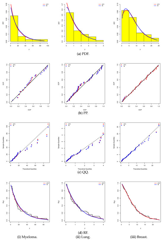
Figure 4. Fitting diagrams for the APE and W models from myeloma, lung, and breast cancer data.

Figure 5 displays the log-likelihood contour plot and the violin boxplot of the APE$\left(\mathit{\vartheta }\right)$ model. Moreover, the contour plot in Figure 5a confirms the existence and uniqueness of the fitted MLEs of $\alpha$ and $\delta$, thereby reinforcing the model’s stability and identifiability. The estimates $\widehat{\alpha }$ and $\widehat{\delta }$ are recommended as robust initial values for subsequent analytical procedures involving this dataset. Figure 5b reveals that the (i) myeloma data is right-skewed, with a wider spread and several high-value outliers, indicating greater variability in survival times; the (ii) lung data is nearly symmetric, with a tighter interquartile range and fewer mild outliers, showing lower variability; and the (iii) breast data is mildly right-skewed, with a moderate spread and fewer outliers, reflecting more consistent survival times.

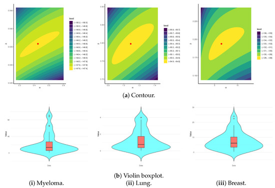
Figure 5. The contour and violin boxplot diagrams for the APE model from myeloma, lung, and breast cancer data.

To assess the theoretical estimation performance of the APE model parameters ($\alpha$, $\delta$, $R\left(x\right)$, and $h\left(x\right)$) together with the BB distribution parameters (${\lambda }_i,i=1,2$), the complete myeloma, lung, and breast cancer datasets were used in a simultaneous, life-testing experiment. These datasets were randomly partitioned into $n=18,22,21$ groups, respectively, each containing $m=2$ units, as shown in Table 12, where starred items denote the first failure in each group. By fixing ${\lambda }_i=1$$(i=1,2)$ and considering different options of k, two artificial P-FFC-BB samples were generated from the myeloma, lung, and breast cancer datasets (see Table 13).

Table 12. Random grouping of myeloma, lung, and breast cancer data.

Myeloma	1	2	3	4	5	6	7	8	9	10	11	12
	${13 }^{★}$	${4 }^{★}$	40	18	10	${5 }^{★}$	65	${10 }^{★}$	66	${5 }^{★}$	${12 }^{★}$	17
	51	16	${8 }^{★}$	${6 }^{★}$	${5 }^{★}$	40	${4 }^{★}$	50	${10 }^{★}$	14	36	${10 }^{★}$
	13	14	15	16	17	18	19	20	21	22	23	24
	${1 }^{★}$	91	${1 }^{★}$	24	${15 }^{★}$	${1 }^{★}$	-	-	-	-	-	-
	88	${6 }^{★}$	23	${5 }^{★}$	18	16	-	-	-	-	-	-
Lung	1	2	3	4	5	6	7	8	9	10	11	12
	1.553	${0.501 }^{★}$	${0.466 }^{★}$	${0.121 }^{★}$	2.444	3.743	${1.099 }^{★}$	${1.219 }^{★}$	1.271	${0.164 }^{★}$	2.416	1.326
	${0.132 }^{★}$	2.830	0.529	0.334	${2.178 }^{★}$	${0.395 }^{★}$	3.978	1.581	${0.458 }^{★}$	0.534	${0.863 }^{★}$	${0.641 }^{★}$
	13	14	15	16	17	18	19	20	21	22	23	24
	2.825	${0.282 }^{★}$	${1.447 }^{★}$	3.658	${0.260 }^{★}$	3.578	${0.203 }^{★}$	0.296	4.003	${0.540 }^{★}$	-	-
	${0.507 }^{★}$	0.644	1.485	${0.696 }^{★}$	2.343	${0.197 }^{★}$	1.589	${0.115 }^{★}$	${0.047 }^{★}$	0.841	-	-
Breast	1	2	3	4	5	6	7	8	9	10	11	12
	${9.40 }^{★}$	4.49	${3.89 }^{★}$	${0.75 }^{★}$	13.98	17.72	${6.96 }^{★}$	7.84	8.81	${1.17 }^{★}$	${5.46 }^{★}$	11.43
	9.77	${1.01 }^{★}$	15.15	4.68	${3.38 }^{★}$	${6.56 }^{★}$	10.57	${3.49 }^{★}$	${6.38 }^{★}$	4.55	6.11	${4.91 }^{★}$
	13	14	15	16	17	18	19	20	21	22	23	24
	13.19	${8.82 }^{★}$	9.24	${2.60 }^{★}$	17.43	${2.42 }^{★}$	1.77	3.01	22.48	-	-	-
	${6.08 }^{★}$	11.49	${5.75 }^{★}$	18.06	${1.37 }^{★}$	9.17	${0.64 }^{★}$	${0.45 }^{★}$	${3.85 }^{★}$	-	-	-

Table 13. Artificial P-FFC-BB samples from myeloma, lung, and breast cancer data.

Myeloma Data
k	i	1	2	3	4	5	6	7	8	9	10	11	12	13	14	15
10	$r_i$	6	0	1	1	0	0	0	0	0	0	-	-	-	-	-
	$y_i$	1	4	4	5	6	6	8	10	10	15	-	-	-	-	-
15	i	1	2	3	4	5	6	7	8	9	10	11	12	13	14	15
	$r_i$	2	0	1	0	0	0	0	0	0	0	0	0	0	0	0
	$y_i$	1	1	1	4	4	5	5	6	6	8	10	10	10	12	13
Lung Data
k	i	1	2	3	4	5	6	7	8	9	10	11	12	13	14	15
10	$r_i$	9	0	2	1	0	0	0	0	0	0	-	-	-	-	-
	$y_i$	0.121	0.132	0.164	0.197	0.395	0.458	0.507	0.540	1.099	1.219	-	-	-	-	-
15	i	1	2	3	4	5	6	7	8	9	10	11	12	13	14	15
	$r_i$	5	0	1	1	0	0	0	0	0	0	0	0	0	0	0
	$y_i$	0.121	0.132	0.164	0.197	0.282	0.395	0.458	0.466	0.507	0.540	0.641	0.863	1.099	1.219	1.447
Breast Data
k	i	1	2	3	4	5	6	7	8	9	10	11	12	13	14	15
10	$r_i$	8	0	2	1	0	0	0	0	0	0	-	-	-	-	-
	$y_i$	0.64	0.75	1.01	1.17	1.37	3.49	3.85	5.46	5.75	6.96	-	-	-	-	-
15	i	1	2	3	4	5	6	7	8	9	10	11	12	13	14	15
	$r_i$	5	0	1	0	0	0	0	0	0	0	0	0	0	0	0
	$y_i$	0.64	0.75	1.01	1.17	1.37	2.60	3.38	3.49	3.85	4.91	5.46	5.75	6.56	6.96	9.40

In progressive censoring studies, the independence assumption between random removals and observed failure times is common because withdrawals are typically driven by administrative or external factors (e.g., patient drop-out or loss to follow-up) rather than the exact time-to-failure of other units.

Using the P-FFC-BB samples (with $k=10$) generated from the myeloma, lung, and breast cancer datasets reported in Table 13, the corresponding Spearman rank correlation statistics (with their associated p-values) between the observed failure times and removal counts are estimated as −0.714 (0.020), −0.678 (0.030), and −0.679 (0.031), respectively. These results indicate a statistically significant negative association: groups with earlier failures tended to have higher numbers of removals. This finding suggests that the assumption of independence between removals and failure times may not hold strictly for these datasets.

In the absence of prior information on the APE parameters $\mathit{\vartheta }$ and the BB $\left(\mathit{\lambda }\right)$ parameters, a vague joint gamma prior with hyperparameters $a_i=b_i=0.001$$(i=1,2,3,4)$ was adopted. Following Algorithm 1, a total of $\mathbb{W}=40,000$ iterations were run, discarding the first ${\mathbb{W}}^{•}=10,000$ iterations as burn-in. Posterior summaries were then obtained for $\alpha$, $\delta$, $R\left(x\right)$, $h\left(x\right)$, and ${\lambda }_i,i=1,2$, including MCMC estimates under both SEL and GEL loss functions with $\tau (=-3,-0.03,+3)$, as well as their 95% BCI/HPD interval estimates. For $x=5,0.1,$ and 1 in the myeloma, lung, and breast cancer datasets, respectively, all estimates of $R\left(x\right)$ and $h\left(x\right)$ were computed. The resulting point estimates (with their Std.Ers) and the 95% interval estimates (with their ILs) are summarized in Table 14 and Table 15. In comparison to classical likelihood-based estimates of $\alpha$, $\delta$, $R\left(x\right)$, $h\left(x\right)$, and ${\lambda }_i,i=1,2$, the point and interval estimation findings developed from the Bayesian approach showed clear superiority, producing smaller Std.Ers and shorter ILs for all parameters.

Table 14. The point estimates of $\alpha$, $\delta$, $R\left(x\right)$, $h\left(x\right)$, and ${\lambda }_i,i=1,2$ from myeloma, lung, and breast cancer datasets.

k	Par.	MLE		SEL		GEL ($\mathit{\tau }=-3$)		GEL ($\mathit{\tau }=-0.03$)		GEL ($\mathit{\tau }=+3$)
		Est.	Std.Er	Est.	Std.Er	Est.	Std.Er	Est.	Std.Er	Est.	Std.Er
Myeloma Data
10	$\alpha$	203.10	11.870	203.10	0.0100	203.10	0.0001	203.10	0.0001	203.10	0.0003
	$\delta$	0.2165	0.0344	0.2160	0.0958	0.2164	0.0049	0.2158	0.0679	0.2151	0.1327
	$R\left(x\right)$	0.9910	0.0021	0.9910	0.0057	0.9910	0.0020	0.9910	0.0019	0.9910	0.0019
	$h\left(x\right)$	0.0130	0.0036	0.0130	0.0099	0.0131	0.0049	0.0129	0.0063	0.0128	0.0178
	${\lambda }_1$	0.3038	0.2486	0.3010	0.2008	0.3024	0.1471	0.3004	0.3420	0.2984	0.5439
	${\lambda }_2$	0.6760	0.3007	0.6741	0.2005	0.6747	0.1295	0.6738	0.2172	0.6729	0.3071
15	$\alpha$	30.280	8.6764	30.280	0.0999	30.280	0.0012	30.280	0.0007	30.280	0.0002
	$\delta$	0.1846	0.0304	0.1840	0.0948	0.1845	0.0039	0.1838	0.0762	0.1831	0.1508
	$R\left(x\right)$	0.7675	0.0538	0.7683	0.1709	0.7687	0.1182	0.7681	0.0619	0.7675	0.0042
	$h\left(x\right)$	0.0869	0.0244	0.0866	0.0784	0.0873	0.0418	0.0863	0.0633	0.0852	0.1723
	${\lambda }_1$	0.0969	0.0840	0.0936	0.1985	0.0975	0.0628	0.0915	0.5407	0.0835	1.3381
	${\lambda }_2$	0.6027	0.2535	0.6019	0.1980	0.6025	0.0199	0.6016	0.1165	0.6006	0.2154
Lung Data
10	$\alpha$	30.400	19.070	30.400	0.0994	30.400	0.0025	30.400	0.0030	30.400	0.0035
	$\delta$	2.2418	0.5181	2.2417	0.1005	2.2418	0.0072	2.2417	0.0139	2.2416	0.0207
	$R\left(x\right)$	0.9665	0.0121	0.9665	0.0019	0.9665	0.0002	0.9665	0.0002	0.9665	0.0002
	$h\left(x\right)$	0.4274	0.1498	0.4274	0.0274	0.4274	0.0010	0.4274	0.0036	0.4273	0.0063
	${\lambda }_1$	0.3081	0.2618	0.3042	0.2034	0.3055	0.2566	0.3036	0.4511	0.3016	0.6528
	${\lambda }_2$	0.6381	0.2931	0.6354	0.2024	0.6360	0.2118	0.6351	0.3058	0.6341	0.4021
15	$\alpha$	24.350	13.558	24.350	0.0994	24.350	0.0024	24.350	0.0030	24.350	0.0036
	$\delta$	1.9574	0.3750	1.9572	0.1005	1.9573	0.0070	1.9572	0.0147	1.9571	0.0225
	$R\left(x\right)$	0.9673	0.0102	0.9673	0.0020	0.9673	0.0002	0.9673	0.0002	0.9673	0.0002
	$h\left(x\right)$	0.4013	0.1198	0.4012	0.0280	0.4013	0.0010	0.4012	0.0039	0.4012	0.0069
	${\lambda }_1$	0.1611	0.1213	0.1560	0.2035	0.1584	0.2679	0.1547	0.6356	0.1507	1.0404
	${\lambda }_2$	0.6246	0.2441	0.6214	0.2028	0.6221	0.2541	0.6211	0.3500	0.6201	0.4483
Breast Data
10	$\alpha$	19.081	27.933	19.081	0.0994	19.081	0.0017	19.081	0.0025	19.081	0.0033
	$\delta$	0.3234	0.1145	0.3231	0.0996	0.3234	0.0043	0.3229	0.0498	0.3225	0.0964
	$R\left(x\right)$	0.9304	0.0374	0.9305	0.0265	0.9305	0.0086	0.9305	0.0075	0.9304	0.0063
	$h\left(x\right)$	0.0927	0.0395	0.0926	0.0416	0.0928	0.0082	0.0925	0.0195	0.0922	0.0479
	${\lambda }_1$	0.3112	0.2629	0.3073	0.2035	0.3086	0.2556	0.3067	0.4483	0.3047	0.6481
	${\lambda }_2$	0.6459	0.2944	0.6432	0.2024	0.6438	0.2108	0.6429	0.3036	0.6419	0.3988
15	$\alpha$	19.656	9.2647	19.656	0.0994	19.656	0.0025	19.656	0.0032	19.656	0.0040
	$\delta$	0.2811	0.0528	0.2808	0.0984	0.2811	0.0025	0.2806	0.0536	0.2801	0.1059
	$R\left(x\right)$	0.9424	0.0157	0.9425	0.0246	0.9425	0.0084	0.9425	0.0074	0.9424	0.0064
	$h\left(x\right)$	0.0746	0.0204	0.0745	0.0372	0.0747	0.0086	0.0744	0.0189	0.0741	0.0470
	${\lambda }_1$	0.0927	0.0817	0.0891	0.1982	0.0932	0.0486	0.0869	0.5792	0.0785	1.4219
	${\lambda }_2$	0.5652	0.2469	0.5645	0.1994	0.5653	0.0078	0.5642	0.0966	0.5631	0.2037

Table 15. The 95% interval estimates of $\alpha$, $\delta$, $R\left(x\right)$, $h\left(x\right)$, and ${\lambda }_i,i=1,2$ from myeloma, lung, and breast cancer datasets.

k	Par.	ACI-NA			ACI-NL			BCI			HPD
		Low.	Upp.	IL	Low.	Upp.	IL	Low.	Upp.	IL	Low.	Upp.	IL
Myeloma Data
10	$\alpha$	179.83	226.36	46.531	181.12	227.75	46.633	203.08	203.12	0.0393	203.08	203.12	0.0392
	$\delta$	0.1491	0.2839	0.1348	0.1586	0.2956	0.1370	0.1973	0.2347	0.0374	0.1973	0.2347	0.0374
	$R\left(x\right)$	0.9870	0.9951	0.0081	0.9870	0.9951	0.0081	0.9899	0.9921	0.0022	0.9899	0.9921	0.0022
	$h\left(x\right)$	0.0060	0.0200	0.0140	0.0076	0.0223	0.0147	0.0111	0.0150	0.0039	0.0111	0.0150	0.0039
	${\lambda }_1$	0.0083	0.7911	0.7827	0.0611	1.5104	1.4493	0.2626	0.3403	0.0777	0.2429	0.3147	0.0718
	${\lambda }_2$	0.0866	1.2654	1.1788	0.2827	1.6166	1.3339	0.6355	0.7135	0.0780	0.5878	0.6600	0.0722
15	$\alpha$	13.275	47.285	34.011	17.269	53.095	35.827	30.260	30.300	0.0390	30.260	30.299	0.0390
	$\delta$	0.1251	0.2441	0.1190	0.1337	0.2548	0.1211	0.1655	0.2026	0.0371	0.1654	0.2025	0.0370
	$R\left(x\right)$	0.6621	0.8729	0.2108	0.6690	0.8804	0.2114	0.7345	0.8013	0.0668	0.7348	0.8015	0.0667
	$h\left(x\right)$	0.0392	0.1347	0.0955	0.0502	0.1506	0.1004	0.0717	0.1024	0.0307	0.0716	0.1022	0.0306
	${\lambda }_1$	0.0068	0.2614	0.2547	0.0177	0.5297	0.5120	0.0553	0.1320	0.0767	0.0512	0.1221	0.0709
	${\lambda }_2$	0.1059	1.0995	0.9936	0.2643	1.3744	1.1100	0.5634	0.6411	0.0777	0.5211	0.5930	0.0719
Lung Data
10	$\alpha$	0.0000	67.777	67.777	8.8904	103.95	95.062	30.381	30.420	0.0390	30.381	30.4201	0.0390
	$\delta$	1.2265	3.2572	2.0308	1.4253	3.5262	2.1009	2.2221	2.2615	0.0394	2.2224	2.2618	0.0394
	$R\left(x\right)$	0.9428	0.9902	0.0474	0.9431	0.9905	0.0474	0.9661	0.9669	0.0007	0.9661	0.9669	0.0007
	$h\left(x\right)$	0.1339	0.7209	0.5870	0.2151	0.8493	0.6343	0.4220	0.4328	0.0108	0.4221	0.4328	0.0107
	${\lambda }_1$	0.0050	0.8212	0.8162	0.0583	1.6292	1.5709	0.2653	0.3438	0.0785	0.2454	0.3180	0.0726
	${\lambda }_2$	0.0636	1.2126	1.1490	0.2594	1.5700	1.3107	0.5963	0.6745	0.0782	0.5516	0.6240	0.0723
15	$\alpha$	0.0000	50.922	50.922	8.1764	72.515	64.339	24.330	24.369	0.0390	24.330	24.369	0.0390
	$\delta$	1.2224	2.6924	1.4700	1.3446	2.8494	1.5048	1.9376	1.9771	0.0394	1.9379	1.9773	0.0394
	$R\left(x\right)$	0.9472	0.9874	0.0402	0.9474	0.9876	0.0402	0.9669	0.9677	0.0008	0.9669	0.9677	0.0008
	$h\left(x\right)$	0.1664	0.6361	0.4697	0.2235	0.7205	0.4970	0.3958	0.4068	0.0110	0.3958	0.4068	0.0110
	${\lambda }_1$	0.0018	0.3989	0.3971	0.0368	0.7050	0.6682	0.1173	0.1948	0.0774	0.1085	0.1802	0.0716
	${\lambda }_2$	0.1461	1.1031	0.9570	0.2904	1.3437	1.0533	0.5825	0.6606	0.0781	0.5388	0.6111	0.0722
Breast Data
10	$\alpha$	0.0000	73.829	73.829	1.0826	336.29	335.21	19.061	19.100	0.0391	19.061	19.1002	0.0390
	$\delta$	0.0990	0.5479	0.4490	0.1616	0.6474	0.4859	0.3036	0.3427	0.0390	0.3036	0.3425	0.0390
	$R\left(x\right)$	0.8571	1.0037	0.1467	0.8599	1.0067	0.1468	0.9252	0.9356	0.0104	0.9252	0.9356	0.0104
	$h\left(x\right)$	0.0153	0.1701	0.1548	0.0402	0.2136	0.1734	0.0846	0.1009	0.0163	0.0845	0.1008	0.0163
	${\lambda }_1$	0.0041	0.8265	0.8224	0.0594	1.6298	1.5704	0.2684	0.3470	0.0786	0.2482	0.3209	0.0727
	${\lambda }_2$	0.0689	1.2230	1.1541	0.2643	1.5782	1.3139	0.6041	0.6823	0.0782	0.5588	0.6311	0.0723
15	$\alpha$	1.4981	37.815	36.317	7.8039	49.511	41.707	19.637	19.676	0.0390	19.637	19.676	0.0390
	$\delta$	0.1777	0.3846	0.2069	0.1946	0.4062	0.2116	0.2616	0.3002	0.0385	0.2617	0.3002	0.0385
	$R\left(x\right)$	0.9116	0.9731	0.0615	0.9121	0.9736	0.0615	0.9376	0.9472	0.0096	0.9375	0.9472	0.0096
	$h\left(x\right)$	0.0347	0.1145	0.0799	0.0437	0.1274	0.0837	0.0674	0.0820	0.0146	0.0673	0.0818	0.0146
	${\lambda }_1$	0.0017	0.2529	0.2512	0.0165	0.5216	0.5051	0.0511	0.1279	0.0768	0.0473	0.1183	0.0710
	${\lambda }_2$	0.0812	1.0491	0.9679	0.2400	1.3307	1.0906	0.5257	0.6038	0.0780	0.4863	0.5585	0.0722

To establish the existence and uniqueness of the MLEs for the parameters of APE $\left(\mathit{\vartheta }\right)$ and BB $\left(\mathit{\lambda }\right)$, based on the P-FFC-BB datasets summarized in Table 13, Figure 6 depicts the log-likelihood contours of $\alpha$, $\delta$, and ${\lambda }_i$ ($i=1,2$). These plots demonstrate that the fitted MLEs (reported in Table 14) for both APE $\left(\mathit{\vartheta }\right)$ and BB $\left(\mathit{\lambda }\right)$ exist and are unique. Using these estimates as initial values, the proposed Markov chains were implemented. To assess the convergence behavior of the simulated 40,000 Markov chain variates for $\alpha$, $\delta$, $R\left(x\right)$, $h\left(x\right)$, and ${\lambda }_i$ ($i=1,2$), we focused on the P-FFC-BB dataset at $k=10$ (as a representative case) from Table 13. Figure 7 presents the corresponding trace plots and posterior density plots for each parameter. In each plot, the solid line denotes the Bayes’ MCMC estimates calculated by the SEL, and the dashed lines represent the 95% BCI bounds. The trace plots indicate that the simulated chains for all parameters exhibit stable and symmetric behavior, suggesting satisfactory convergence. To further validate this, we summarized key descriptive statistics based on the remaining 40,000 post-burn-in samples for each parameter (see Table 16). These numerical summaries reinforce the visual evidence from Figure 7, providing additional support for convergence and distributional stability across all monitored parameters.

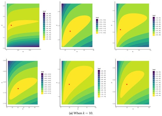
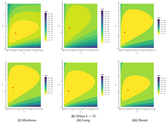
Figure 6. Contours of APE($\alpha$,$\delta$) and BB(${\lambda }_1$,${\lambda }_2$) distributions from myeloma, lung, and breast cancer datasets.

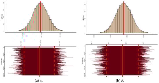
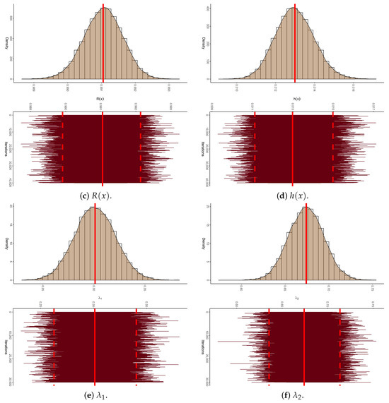
Figure 7. The density (with its Gaussian curve) and trace diagrams of $\alpha$, $\delta$, $R\left(x\right)$, $h\left(x\right)$, and ${\lambda }_i,i=1,2$ from myeloma data.

Table 16. Statistical summary for MCMC iterations of $\alpha$, $\delta$, $R\left(x\right)$, $h\left(x\right)$, and ${\lambda }_i,i=1,2$ from myeloma, lung, and breast cancer data.

k	Par.	Mean	Mode	${\mathbb{Q}}_1$	${\mathbb{Q}}_2$	${\mathbb{Q}}_3$	Std.Dv.	Skew.
Myeloma Data
10	$\alpha$	203.099	203.100	203.092	203.099	203.105	0.01000	0.02287
	$\delta$	0.21600	0.20681	0.20958	0.21599	0.22246	0.00957	0.00602
	$R\left(x\right)$	0.99105	0.99078	0.99067	0.99106	0.99143	0.00057	−0.10196
	$h\left(x\right)$	0.01299	0.01203	0.01231	0.01296	0.01364	0.00099	0.14546
	${\lambda }_1$	0.30105	0.27234	0.28753	0.30088	0.31455	0.01989	0.03086
	${\lambda }_2$	0.67413	0.66392	0.66041	0.67418	0.68760	0.01996	0.00436
15	$\alpha$	30.2800	30.2574	30.2733	30.2800	30.2868	0.00999	0.00328
	$\delta$	0.18404	0.17197	0.17767	0.18406	0.19030	0.00947	0.00460
	$R\left(x\right)$	0.76829	0.75334	0.75708	0.76839	0.77987	0.01707	−0.05622
	$h\left(x\right)$	0.08663	0.07673	0.08127	0.08650	0.09173	0.00784	0.11859
	${\lambda }_1$	0.09356	0.05305	0.08036	0.09350	0.10673	0.01957	0.03300
	${\lambda }_2$	0.60187	0.56653	0.58858	0.60183	0.61512	0.01978	0.00326
Lung Data
10	$\alpha$	30.4004	30.3974	30.3936	30.4004	30.4071	0.00994	0.01319
	$\delta$	2.24172	2.23777	2.23491	2.24171	2.24851	0.01005	0.01921
	$R\left(x\right)$	0.96649	0.96656	0.96637	0.96649	0.96662	0.00019	−0.02512
	$h\left(x\right)$	0.42736	0.42630	0.42550	0.42735	0.42921	0.00274	0.02841
	${\lambda }_1$	0.30424	0.26931	0.29085	0.30406	0.31766	0.01997	0.02610
	${\lambda }_2$	0.63538	0.57834	0.62188	0.63529	0.64890	0.02006	−0.00381
15	$\alpha$	24.3497	24.3467	24.3429	24.3497	24.3564	0.00994	0.01330
	$\delta$	1.95725	1.95330	1.95044	1.95724	1.96404	0.01005	0.01943
	$R\left(x\right)$	0.96729	0.96736	0.96715	0.96729	0.96742	0.00020	−0.02510
	$h\left(x\right)$	0.40125	0.40017	0.39935	0.40123	0.40313	0.00280	0.02858
	${\lambda }_1$	0.15597	0.12230	0.14279	0.15592	0.16923	0.01969	0.01151
	${\lambda }_2$	0.62143	0.56482	0.60797	0.62134	0.63495	0.02003	−0.00888
Breast Data
10	$\alpha$	19.0805	19.0646	19.0738	19.0805	19.0872	0.00994	0.01214
	$\delta$	0.32308	0.30984	0.31634	0.32307	0.32979	0.00995	0.01863
	$R\left(x\right)$	0.93046	0.92912	0.92868	0.93047	0.93226	0.00265	−0.05226
	$h\left(x\right)$	0.09257	0.08704	0.08973	0.09253	0.09534	0.00416	0.07822
	${\lambda }_1$	0.30733	0.27238	0.29392	0.30715	0.32075	0.01998	0.02607
	${\lambda }_2$	0.64317	0.58611	0.62968	0.64307	0.65669	0.02006	−0.00431
15	$\alpha$	19.6564	19.6376	19.6497	19.6564	19.6631	0.00994	0.01030
	$\delta$	0.28077	0.26876	0.27410	0.28075	0.28740	0.00983	0.02649
	$R\left(x\right)$	0.94246	0.94120	0.94081	0.94248	0.94413	0.00246	−0.06297
	$h\left(x\right)$	0.07450	0.06996	0.07196	0.07446	0.07699	0.00372	0.09104
	${\lambda }_1$	0.08914	0.06024	0.07601	0.08899	0.10222	0.01949	0.04639
	${\lambda }_2$	0.56455	0.54253	0.55106	0.56443	0.57794	0.01993	0.01518

7. Conclusions

In this work, we examined a novel alpha-powering model based on the exponential distribution within the framework of the P-FFC-BB removal plan. This contribution provides a flexible and realistic mechanism for capturing uncertainty in unit withdrawals, a prevalent challenge in reliability and biomedical studies. Comprehensive inference procedures were developed, including both maximum likelihood and Bayesian estimation methods. To address the intractability of the posterior distributions under squared-error and generalized entropy loss functions, a tailored Metropolis–Hastings algorithm was implemented, enabling accurate approximation of posterior summaries and credible intervals. To evaluate the performance of the proposed estimators, we conducted an extensive Monte Carlo simulation study, systematically assessing the effects of varying censoring levels, prior specifications, and group sizes. The simulation results revealed that Bayesian methods—particularly those based on asymmetric loss functions with informative priors—outperform the classical approach, yielding more accurate and stable estimates under complex censoring scenarios. Furthermore, asymptotic confidence intervals and Bayesian credible intervals have been derived and demonstrated satisfactory coverage probabilities across diverse settings. The practical relevance of the proposed model has been validated through applications to three real-world survival datasets from myeloma, lung, and breast cancer patients, where progressive censoring and drop-out variability are inherently present. In all cases, the proposed model exhibited superior goodness of fit, predictive reliability, and improved hazard rate estimation, underscoring its robustness in modeling complex survival mechanisms. While classical methods, such as the Kaplan–Meier estimator, Cox proportional hazards model, and Weibull-based parametric approaches, are well-established for right-censored data, they do not naturally accommodate the progressive first-failure censoring scheme with the stochastic beta–binomial removals considered here. The proposed framework specifically addresses this complexity by deriving tractable likelihoods and flexible hazard structures under such censoring, providing insights beyond the reach of conventional methods. Future work may include empirical comparisons with these classical approaches to highlight further the contexts where our method offers distinct advantages. Future research directions include extending the proposed framework to other baseline distributions with non-monotonic hazard rates, incorporating covariate effects within a regression structure, and exploring accelerated life-testing designs under similar censoring schemes. Future research could extend the proposed censoring framework to other flexible lifetime models—such as log-logistic, log-normal, generalized gamma, or Burr families—to better capture non-monotonic and heavy-tailed hazard structures.

References

- Wu, J.W.; Hung, W.L.; Chen, C.Y. Approximat MLE of the scale parameter of the truncated Rayleigh distribution under the first failure-censored data. J. Inf. Optim. Sci. 2004, 25, 221–235. [Google Scholar]
- Balasooriya, U. Failure–censore reliability sampling plans for the exponential distribution. J. Stat. Comput. Simul. 1995, 52, 337–349. [Google Scholar] [CrossRef]
- Balakrishnan, N.; Cramer, E. The Art of Progressive Censoring. Statistics for Industry and Technology; Springer: Birkhäuser, Germany; New York, NY, USA, 2014. [Google Scholar]
- Huang, S.R.; Wu, S.J. Estimation of Pareto distribution under progressive first-failure censoring with random removals. J. Chin. Stat. Assoc. 2011, 49, 82–97. [Google Scholar]
- Ashour, S.K.; El-Sheikh, A.A.; Elshahhat, A. Inference for Weibull parameters under progressively first-failure censored data with binomial random removals. Stat. Optim. Inf. Comput. 2021, 9, 47–60. [Google Scholar] [CrossRef]
- Elshahhat, A.; Sharma, V.K.; Mohammed, H.S. Statistical analysis of progressively first-failure censored data via β-binomial removals. AIMS Math. 2023, 8, 22419–22446. [Google Scholar] [CrossRef]
- Mahdavi, A.; Kundu, D. A new method for generating distributions with an application to exponential distribution. Commun. Stat.-Theory Methods 2017, 46, 6543–6557. [Google Scholar] [CrossRef]
- Salah, M.M. On Progressive Type-II Censored Samples from Alpha Power Exponential Distribution. J. Math. 2020, 2020, 2584184. [Google Scholar] [CrossRef]
- Salah, M.M.; Ahmed, E.A.; Alhussain, Z.A.; Ahmed, H.H.; El-Morshedy, M.; Eliwa, M.S. Statistica inferences for type-II hybrid censoring data from the alpha power exponential distribution. PLoS ONE 2021, 16, e0244316. [Google Scholar] [CrossRef]
- Alotaibi, R.; Elshahhat, A.; Rezk, H.; Nassar, M. Inference for alpha power exponential distribution using adaptive progressively type-II hybrid censored data with applications. Symmetry 2022, 14, 651. [Google Scholar] [CrossRef]
- Elbatal, I.; Nassar, M.; Ben Ghorbal, A.; Diab, L.S.G.; Elshahhat, A. Reliabilit analysis and its applications for a newly improved type-II adaptive progressive alpha power exponential censored sample. Symmetry 2023, 15, 2137. [Google Scholar] [CrossRef]
- Elsherpieny, E.A.; Abdel-Hakim, A. Statistica analysis of Alpha-Power exponential distribution using unified Hybrid censored data and its applications. Comput. J. Math. Stat. Sci. 2025, 4, 283–315. [Google Scholar]
- Singh, S.K.; Singh, U.; Sharma, V.K. Expecte total test time and Bayesian estimation for generalized Lindley distribution under progressively Type-II censored sample where removals follow the beta-binomial probability law. Appl. Math. Comput. 2013, 222, 402–419. [Google Scholar]
- Kaushik, A.; Singh, U.; Singh, S.K. Bayesia inference for the parameters of Weibull distribution under progressive Type-I interval censored data with beta-binomial removals. Commun. Stat.-Simul. Comput. 2017, 46, 3140–3158. [Google Scholar] [CrossRef]
- Sangal, P.K.; Sinha, A. Classical estimation in exponential power distribution under Type-I progressive hybrid censoring with beta-binomial removals. Int. J. Agric. Stat. Sci. 2021, 17, 1973–1988. [Google Scholar]
- Usta, I.; Gezer, H. Paramete estimation in Weibull distribution on progressively Type-II censored sample with beta-binomial removals. Econ. Bus. J. 2016, 10, 505–515. [Google Scholar]
- Vishwakarma, P.K.; Kaushik, A.; Pandey, A.; Singh, U.; Singh, S.K. Bayesia estimation for inverse Weibull distribution under progressive Type-II censored data with beta-binomial removals. Austrian J. Stat. 2018, 47, 77–94. [Google Scholar] [CrossRef]
- Greene, W.H. Econometric Analysis, 4th ed.; Prentice-Hall: New York, NY, USA, 2000. [Google Scholar]
- Kundu, D. Bayesia inference and life testing plan for the Weibull distribution in presence of progressive censoring. Technometrics 2008, 50, 144–154. [Google Scholar] [CrossRef]
- Dey, S.; Elshahhat, A.; Nassar, M. Analysi of progressive type-II censored gamma distribution. Comput. Stat. 2023, 38, 481–508. [Google Scholar] [CrossRef]
- Martz, H.F.; Waller, R.A. Bayesian Reliability Analysis; Wiley and Sons: New York, NY, USA, 1982. [Google Scholar]
- Dey, D.K.; Ghosh, M.; Srinivasan, C. Simultaneou estimation of parameters under entropy loss. J. Stat. Plan. Inference 1987, 15, 347–363. [Google Scholar] [CrossRef]
- Henningsen, A.; Toomet, O. maxLik: A package for maximum likelihood estimation in R. Comput. Stat. 2011, 26, 443–458. [Google Scholar] [CrossRef]
- Plummer, M.; Best, N.; Cowles, K.; Vines, K. CODA: Convergence diagnosis and output analysis for MCMC. R News 2006, 6, 7–11. [Google Scholar]
- Collett, D. Modelling Survival Data in Medical Research; Chapman and Hall/CRC: Boca Raton, FL, USA, 2023. [Google Scholar]
- Lawless, J.F. Statistical Models and Methods for Lifetime Data; John Wiley and Sons: New York, NY, USA, 2011. [Google Scholar]
- Royston, P.; Altman, D.G. Externa validation of a Cox prognostic model: Principles and methods. BMC Med. Res. Methodol. 2013, 13, 33. [Google Scholar] [CrossRef]
- Bourguignon, M.; Silva, R.B.; Cordeiro, G.M. The Weibull-G family of probability distributions. J. Data Sci. 2014, 12, 53–68. [Google Scholar] [CrossRef]
Disclaimer/Publisher’s Note: The statements, opinions and data contained in all publications are solely those of the individual author(s) and contributor(s) and not of MDPI and/or the editor(s). MDPI and/or the editor(s) disclaim responsibility for any injury to people or property resulting from any ideas, methods, instructions or products referred to in the content. |
© 2025 by the authors. Licensee MDPI, Basel, Switzerland. This article is an open access article distributed under the terms and conditions of the Creative Commons Attribution (CC BY) license (https://creativecommons.org/licenses/by/4.0/).