Abstract
This study investigates the adoption of blockchain technology (BCT) and financing decisions for capital-constrained manufacturers in live streaming supply chains, where product quality information is asymmetric. Although BCT can improve information transparency and consumer trust, its high cost hinders widespread adoption. Based on supply chain financing theory, this research uses a game-theoretic model with linear demand to analyze manufacturers’ BCT adoption and financing strategies under different capital conditions, comparing four scenarios: non-adoption and non-financing (NN), adoption and non-financing (NB), adoption with loan financing from Multi-Channel Networks (MCNs) (LB), and adoption with investment cost-sharing financing from MCNs (CB). Results show that BCT adoption increases market demand and manufacturer profits. The LB strategy is optimal when the manufacturer has sufficient capital and the MCN has a low-investment cost-sharing ratio. In contrast, CB is preferred when the MCN bears a higher share of investment costs, regardless of the manufacturer’s capital. The manufacturer’s financing choice also influences MCN cooperation: MCNs favor CB under high commission rates and low cost-sharing ratios but prefer NB if investment costs are high. These results suggest that manufacturers should select financing based on their capital and cost-sharing terms, while MCNs can adjust cooperation strategies according to commission rates and cost-sharing levels.
Keywords:
blockchain technology; traceability; supply chain financing; live-streaming supply chain; stackelberg game MSC:
91-10
1. Introduction
1.1. Background and Motivation
In live streaming commerce, as collaborations between manufacturers and multi-channel networks (MCNs) become increasingly close, product quality has emerged as a pivotal element in their partnership [1]. For instance, Meione, leveraging stringent product selection criteria and influencer resources, partnered with the smart home appliance brand Yunjing to maintain strict quality control throughout the process. This collaboration garnered broad consumer recognition and significantly boosted product sales. High product quality is critical in building consumer trust, shaping brand image, and stimulating market demand [2]. However, within the actual operation of live streaming supply chains (LSCs), more accurate product quality information is typically held by manufacturers rather than by MCNs or end consumers [3]. Motivated by informational advantages and various interests, manufacturers may conceal key quality information, adversely affecting information-disadvantaged parties such as MCNs and end consumers. This situation exemplifies quality information asymmetry. Such incidents frequently occur in practice, as cases involving Three Squirrels’ “preserved pork dish” and Mei Cheng’s “mooncakes” demonstrate. These events significantly damaged the brand’s reputation and severely eroded consumer trust.
Due to the complexity and high cost of product quality inspection, it is difficult for MCNs to fully evaluate the quality of manufacturers’ products [4]. Meanwhile, the inability of consumers to inspect products before purchase has led to an increase in low-quality goods and more frequent safety incidents. For example, in 2021, some Three Squirrels products were found to have abnormal peroxide levels, indicating spoilage and potential health risks. Additionally, in 2025, Yang Mingyu Braised Chicken Rice was exposed for serious food safety violations, arousing public concern. These issues are caused by asymmetric product information, harm consumers’ immediate interests, and damage high-quality manufacturers’ reputation and long-term profitability [5]. Consequently, effectively disclosing product quality information has become an urgent issue for manufacturers committed to high standards and sustainable development.
To effectively disclose product quality information, blockchain technology (BCT), characterized by its decentralization and data immutability, demonstrates significant potential for application in supply chain management [6]. In LSCs, using BCT to disclose product quality information and track full life-cycle data can enhance consumer trust and stimulate market demand, creating additional business opportunities for manufacturers and MCNs [7]. Empirical studies and case evidence confirm that BCT enhances transparency. Furthermore, studies by Guo et al. [8] and Caliskan et al. [9] demonstrate that BCT effectively enhances the traceability of product information and quality transparency. This conclusion is also supported by practical applications: for instance, in the collaboration between Wuliangye and AntChain, a unique and immutable digital identity based on BCT, was assigned to each bottle of premium liquor. By scanning the QR code, consumers can trace complete information across all stages—from raw material procurement and brewing processes to quality inspection and logistics. In this study, BCT adoption is considered to have two main effects on manufacturers. First, it increases supply chain transparency and credibility [10], which helps protect the economic interests of quality-focused manufacturers and expands their market demand. Notably, 84% of consumers are willing to pay a 5% premium for products with transparent labeling [11]. This study examines how consumer perceptions of product quality shift after BCT implementation to capture resulting changes in market demand. Second, BCT-based traceability—measured in this research by the level of BCT adoption—strengthens consumer trust, thereby improving loyalty, repurchase intention, and manufacturer reputation [12]. A prominent example is Walmart, where all products are traceable via QR codes that provide full details from raw materials to distribution. More complete traceability information further enhances consumer trust. Accordingly, this study incorporates two key factors: consumers’ initial quality perceptions and the manufacturer’s level of BCT implementation.
However, the widespread adoption of BCT faces multiple challenges, including regulatory uncertainties, technical limitations, divergent user learning outcomes, and related network effects. Among these, financial constraints are a significant barrier for manufacturers seeking to adopt BCT [13]. This is especially evident in an increasingly volatile global economy—exacerbated by the COVID-19 pandemic and subsequent recessions—which has intensified financial pressure on many firms. Manufacturers must seek effective financing strategies to overcome these barriers and promote BCT implementation. Most small- and medium-sized enterprises (SMEs) face difficulties securing bank loans due to their small scale, insufficient assets, lack of collateral, and limited credit history [14]. Moreover, bank financing has become more costly for SMEs since the 2008 financial crisis. Consequently, many turn to supply chain financing (SCF) as an alternative [15]. This study focuses on financing through MCNs within LSCs. MCNs can support manufacturers via two financing modes: loans or cost-sharing. Loans form a debt-based relationship with the MCN as lender, while cost-sharing represents a strategic partnership, often governed by incentive contracts. These approaches reduce financial burdens and encourage BCT adoption and quality improvement, promoting long-term business sustainability. Accordingly, this study investigates BCT adoption and financing decisions for financially constrained manufacturers in LSCs.
1.2. Research Questions and Major Findings
Based on the above background analysis, this study aims to address the following core research questions:
Q1: In LSCs, should manufacturers seek financing from MCNs to adopt BCT? If so, which strategy is more appropriate—loan financing or investment cost-sharing? What are the key factors influencing their decisions regarding BCT adoption and financing?
Q2: How do different financing strategies affect product pricing and the evolution of market demand when manufacturers introduce BCT?
Q3: How do manufacturers’ financing choices influence the profitability of MCNs?
To address these questions, two scenarios are first explored. One pertains to the BCT adoption strategy of manufacturers with unrestricted capital, and the other concerns the financing strategy for BCT adoption by manufacturers with constrained capital. Based on this, the equilibrium results are compared before and after the manufacturer’s adoption of BCT. This comparison aims to probe into the manufacturer’s motivation for adopting BCT, ascertain the optimal BCT adoption level, and investigate the evolution trend of its pricing strategy and profit level. We use backward induction to derive equilibrium solutions across scenarios. Taking the LB strategy as an example: the manufacturer’s optimal price is determined first, followed by the influencer’s optimal effort level, and finally the manufacturer’s optimal BCT adoption level. This sequence yields all equilibrium outcomes for the strategy. It is worth noting that Stackelberg game models are widely applied in operations and supply chain finance research, providing a rigorous and practical mathematical framework for analyzing sequential decision-making and strategic interactions among firms [16]. Subsequently, the impacts of key factors, including the manufacturer’s initial capital and MCN’s investment cost-sharing ratio, on selecting its optimal financing strategy are comprehensively considered. Furthermore, the choice of financing strategy by the manufacturer will influence the profit and loss situation of MCN, which is further explored.
We obtain several novel findings. Regarding Q1, BCT adoption improves the influencer’s effort level in LSCs, leading to higher retail prices, greater market demand, and increased profit for the manufacturer. However, due to high adoption costs, financially constrained manufacturers require financing from MCNs to implement BCT profitably. Further analysis shows that the choice of financing strategy depends mainly on initial capital and the cost-sharing ratio. Specifically, the LB strategy is preferred when the manufacturer has sufficient initial capital and the MCN offers a relatively low investment cost-sharing ratio. This conclusion contrasts with, who found the CB strategy more beneficial for suppliers under similar conditions. The difference arises from incorporating multidimensional factors such as the initial funding gap, financing costs, and demand enhancement effects. Notably, the CB strategy becomes optimal when the manufacturer’s initial capital is low, or even if sufficient, but the investment cost-sharing ratio is high. For Q2, CB and LB strategies affect the manufacturer’s pricing and market demand differently from the NB strategy. Under the LB strategy, the retail price of the product and market demand decrease. In contrast, the CB strategy leads to higher pricing and stronger market performance. Further comparison shows that price and demand are higher under CB than under LB, which is consistent with earlier findings. This difference may be because, unlike LB, the CB strategy does not involve fixed repayments or interest burdens.
As a result, the manufacturer faces less financial pressure, strengthening its motivation and confidence to improve product quality and expand market presence, ultimately increasing both price and sales volume. Regarding Q3, our study shows that the effect of the manufacturer’s financing strategy on the MCN’s profit depends on both the MCN’s investment cost-sharing ratio and the commission rate. Notably, when the commission rate is low or high but coupled with a high cost-sharing ratio, both financing strategies reduce the MCN’s profit. In such cases, the MCN would prefer cooperation under the NB strategy. This conclusion differs from the view of Ma et al. [17], who found that under high commission rates, e-commerce platforms (equivalent to MCNs) are more willing to provide loans to retailers (equivalent to manufacturers). The discrepancy arises because their study considered only loan financing, whereas our research incorporates investment cost-sharing and loan-based financing. Therefore, for MCNs to ensure profitability, it is essential to carefully consider the interplay between the commission rate and the investment cost-sharing ratio.
1.3. Contribution Statement and Structure of This Paper
This study contributes to both academic and practical domains. To our knowledge, it is the first time that BCT adoption and financing strategy selection in LSCs have been examined academically. This work extends previous research by analyzing each strategy’s operational boundaries and contextual effectiveness under “BCT + SCF” dynamic market conditions. It offers manufacturers a decision-making framework for BCT adoption and financing aligned with specific contexts. Practically, the findings provide actionable guidance for firms introducing BCT and selecting financing strategies in LSCs. For example, BCT adoption can enhance the effort levels of influencers under MCNs, leading to higher retail prices, greater market demand, and increased manufacturer profits. Moreover, when initial capital is sufficient and the MCN’s investment cost-sharing ratio is low, the LB strategy is preferable; when capital is scarce—or even sufficient, but the cost-sharing ratio is high—the CB strategy should be selected.
The remainder of this paper is structured as follows: Section 2 reviews relevant literature, while Section 3 details the model and defines key parameters. Section 4 analyzes four strategic scenarios across two distinct settings. Section 5 compares manufacturers’ optimal financing strategies under these scenarios, and Section 6 examines how manufacturers’ financing decisions affect MCN profitability. Section 7 concludes with findings, managerial insights, and future research directions. All equilibrium solutions, thresholds, and proofs appear in the Appendix A, Appendix B, Appendix C and Appendix D.
2. Literature Review
Our research centers on investigating the problem of how capital-constrained manufacturers adopt BCT and choose their financing strategies within LSCs. This research is primarily associated with the following two research areas: (i) supply chain financing (SCF) and (ii) BCT in livestreaming supply chains (LSCs).
2.1. SCF
SCF has attracted extensive scholarly attention as an emerging and rapidly developing field. A primary research focus within this area is diversified financing models [18]. Standard financing methods identified in the literature include bank loans, retailer trade credit, platform financing, and financing services provided by 3PL and 4PL providers. Bank loans, a classic form of external financing, play a key role in easing corporate financial pressures and mitigating risks [19]. Meanwhile, manufacturers or suppliers with limited internal funds often utilize options such as retailer trade credit [20]. Scholars have further expanded this line of inquiry by exploring additional financing channels—platform, 3PL, and 4PL financing—to identify optimal solutions. For example, Mandal, Basu, Choi, and Rath [14] studied how competition among third-party sellers influences their choice between platform financing and bank loans. Tang et al. [21] examined settings where 3PL providers offer logistics and financial support, analyzing the best financing and sales channel choices for capital-constrained manufacturers when selecting bank and 3PL loans. With continued innovation in financing models and evolving consumer shopping experiences, new approaches such as e-commerce platform financing and 4PF have also emerged, offering firms a broader range of options to address capital shortages.
In addition to the financing methods discussed earlier, this research focused on investment cost-sharing as an effective means of alleviating capital constraints, a matter of great significance in supply chain management [22]. Taking a dual-channel supply chain as an example, Niu et al. [23] introduced two incentive mechanisms—advance payments and investment cost-sharing—to address supplier capital shortages and uncertainties in quality improvement, thereby encouraging higher product quality. The research scope has also been extended to green supply chains. Shen et al. [24] compared pricing decisions for green products under cost-sharing mechanisms and found that this approach can significantly enhance product sustainability and supply chain profitability in uncertain markets. Furthermore, Cao, He, Liu, Huang, and Zhang [22] demonstrated that while cost-sharing contracts can alleviate financial pressure and improve supply chain efficiency, enterprises must carefully determine the cost-sharing ratio to ensure desired outcomes.
In conclusion, while prior research on SCF has primarily focused on capital providers such as banks, retailers, and platforms, the potential role of MCNs as financiers within LSCs has been overlooked. Practical cases, such as NetEase Media’s support for Wanmi Culture in team expansion and overseas branding, demonstrate that MCNs can effectively provide financial assistance. This study expands existing research by proposing, for the first time, that MCNs can act as lenders—offering either loans or investment cost-sharing—to alleviate manufacturers’ capital shortages during BCT adoption. We also examine how manufacturers’ financing choices affect MCN profits and influence MCNs’ willingness to cooperate. Notably, when the commission rate is high but the MCN’s cost-sharing ratio is low, the CB strategy increases MCN profits, whereas the LB strategy reduces them. As a result, MCNs prefer cooperating under the CB strategy under these conditions. This finding contrasts with Chang et al. [25], who concluded that financing creates misaligned manufacturer incentives under high commission rates. The key distinction lies in their exclusive focus on platform-provided loans, while our study incorporates both investment cost-sharing and loan offerings by MCNs.
2.2. BCT in LSCs
Due to its ability to enhance data transparency and traceability, BCT has demonstrated broad application potential across areas such as finance, supply chain management, and food safety, driving its rapid development [26]. Literature relevant to our research falls mainly into two categories: one focuses on decision-making related to BCT adoption in LSCs, and the other centers on its specific applications within LSCs.
Research on BCT adoption has primarily focused on two approaches: empirical investigation and theoretical modeling. From an empirical perspective, studies have identified factors influencing BCT adoption and its positive effects on innovation and performance. For example, Flovik et al. [27] used a hierarchical process to analyze data on organizational barriers and facilitators of BCT integration. Jasrotia et al. [28] showed that BCT adoption improves environmental performance, while other studies indicate it enhances operational efficiency and promotes innovation [29]. These findings affirm that multiple factors influence BCT adoption and contribute positively to enterprise development. From a theoretical standpoint, BCT is recognized for reducing transaction costs, increasing supply chain transparency, and improving product quality, leading more firms to consider its implementation [30]. However, real-world adoption remains inconsistent. Jiang et al. [31] examined how tax differences and investment costs affect adoption willingness, noting that high costs inhibit manufacturer engagement. Fang, Chi, Fan, and Choi [6] further explored investment decisions under cost-sharing models and found that commission rates significantly influence supply chain members’ choices. As BCT gains traction in the livestreaming commerce sector, its integration with LSCs to enhance market competitiveness has become a growing academic focus [32].
Although the adoption of BCT faces challenges such as learning effects, network externalities, and consumer barriers, this study focuses on how capital-constrained manufacturers in livestreaming commerce can adopt BCT and develop financing strategies. Existing research mainly explores BCT’s role in improving product traceability, facilitating financing, and enhancing supply chain trust. Regarding product traceability, BCT ensures the authenticity and reliability of product origins [33]. For instance, Iyengar, Saleh, Sethuraman, and Wang [33] demonstrated from a manufacturer’s perspective how BCT enables targeted recalls of defective products, reducing procurement risks and improving overall welfare. From the retailer’s viewpoint, Liu, Zhou, Hu, and Zhong [7] showed that BCT enhances traceability, decreases product returns in livestreaming sales, and strengthens consumer trust. Further expanding this line of research, Liu et al. [34] analyzed how MCNs can use BCT traceability to transmit accurate data signals to retailers, thereby supporting retailer decisions. Regarding financing and supply chain trust, Jiang et al. [35] developed a blockchain-based trust transmission model in supply chain finance, offering a new trust evaluation method for SMEs. Wu, Xu, Zhao, and Zhu [13] addressed information asymmetry and low trust in green supply chain management (GSCM) by modeling a capital-constrained manufacturer and retailer to evaluate BCT’s impact on financing strategies. Guo, Feng, Wang, Zhou, and Liu [8] extended the research to contract farming supply chains (CFSC), investigating how platforms can use BCT to boost customer trust and offer financial services, opening new pathways in this field.
In summary, while the existing literature has focused on adopting and applying BCT, this study takes a different approach. We examine manufacturers committed to producing high-quality products who, due to financial constraints, seek financing from their MCN partners within livestreaming supply chains to adopt BCT. This allows them to leverage BCT’s “demand–expansion effect”—a new perspective not previously studied—where BCT adoption encourages greater consumer purchasing. We analyze two financing strategies provided by MCNs: the CB and LB strategies, aiming to identify the manufacturer’s optimal financing decision and evaluate its impact on MCN profitability. The LB strategy is optimal when the manufacturer has sufficient initial capital and the MCN offers a low-investment cost-sharing ratio. This conclusion contrasts with Niu, Chao, Liu, Zhang, and Luo [23], who found the CB strategy more beneficial for manufacturers under buyer financial support, and Cao, He, Liu, Huang, and Zhang [22], who favored the CB strategy below a certain cost-sharing threshold in semiconductor supply chains. The difference stems from our distinct research context—livestreaming supply chains—where BCT adoption level is treated as an endogenous variable, and our model incorporates multidimensional factors such as the manufacturer’s initial funding gap, financing cost fluctuations, and demand enhancement effects driven by BCT and influencers. This integrated approach enhances the relevance and applicability of our findings.
2.3. Research Gap
We summarize the differences between our work and the related research work in Table 1, highlighting the gaps and underscoring our contributions.

Table 1.
Differences between this paper and the most related papers.
As evident from Table 1, Cui, Gaur, and Liu [30] and Caliskan, Idug, Gligor, and Hong [9] have factored BCT into their research. Liu, Zhou, Hu, and Zhong [7] and Xu, Chen, Hou, Cheng, Yu, and Zhou [32] delved into the adoption and application of BCT within LSCs. However, they did not explore which financing strategies manufacturers should adopt or apply BCT when facing financial limitations. Similarly, Mandal, Basu, Choi, and Rath [14] and Tang, Xu, Chen, and Zhang [21] scrutinized loan financing strategies for manufacturers operating under limitations on finances. Still, the outcomes of cost-sharing and BCT were not taken into account. Moreover, while Niu, Chao, Liu, Zhang, and Luo [23] and Cao, He, Liu, Huang, and Zhang [22] considered cost-sharing, they overlooked the other factors. Drawing on these insights and aligning with real-world practices, we have integrated livestreaming, BCT, loan financing, and investment cost-sharing financing into our model. In current financing practice, these two financing models are not only widely applied but also highly representative. Incorporating them into the model helps clarify the core strategic interactions between the manufacturer and the MCN following the adoption of BCT. Furthermore, focusing on MCN-involved financing approaches closely aligns with the emerging trend of influence-driven credit mechanisms in the livestreaming e-commerce sector, highlighting strong contextual relevance and giving this study distinct novelty. We investigate whether financially constrained manufacturers in LSCs should adopt BCT, which financing strategy is optimal, and how this choice affects MCN profitability. To our knowledge, this specific topic has not been covered in existing literature. Our research extends the knowledge on BCT adoption and offers practical insights for businesses seeking financing solutions under capital constraints.
3. Model
3.1. Model Description
This paper focuses on the impact of financing strategies (including MCN loans and investment cost-sharing) on manufacturers’ BCT adoption decisions and financing choices. The research is set in an LSC context consisting of a high-quality manufacturer (M), a multi-channel network (MCN (L)) engaged in live-streaming sales, and multiple consumers. The manufacturer is responsible for production and partners with influencers affiliated with the MCN to sell products to end consumers through LSCs. Within this LSCs, a salient issue is quality information asymmetry: product quality information is privately held by the manufacturer, who may be incentivized to alter such information. This information asymmetry not only potentially harms the interests of the MCN and consumers but also undermines their trust in high-quality manufacturers, thereby posing a threat to the manufacturer’s own benefits. In light of this, to safeguard its reputation and economic returns, the high-quality manufacturer is incentivized to adopt BCT to disclose its private product quality information.
Manufacturers typically achieve product traceability in industrial applications of BCT by deploying distributed monitoring and data collection equipment across various supply chain nodes. A representative example is Nestlé’s traceability solution for its Zoegas coffee brand, which involves installing IoT sensors and data interfaces at critical stages such as coffee cultivation, processing, and logistics [6]. Building on this practical framework, this study defines the array of data acquisition terminals deployed throughout the supply chain as the “BCT traceability network density”. The intensity of its physical deployment directly reflects the level of BCT adoption, denoted by the variable . A denser network layout enables the BCT system to capture more dimensions of traceability data, thereby enhancing information transparency and tamper-resistance, which corresponds to a higher level of BCT application. Following the approach widely adopted in existing studies [31], we use a quadratic cost function to simulate the cost characteristics of manufacturers’ investment in BCT (including expenses for technological development, system maintenance, certification, etc.) to capture the diseconomies of scale in the expansion of BCT infrastructure: that is, for every one-unit increase in the adoption level , the marginal cost correspondingly increases, implying that the cost of extending transparency gradually rises. For example, when constructing full-chain traceability for Feihe infant formula and expanding from basic information uploading to full-link coverage, addressing challenges such as data access, compliance, and security is necessary, leading to an accelerated cost increase. Here, represents the cost coefficient of BCT adoption.
It is noteworthy that manufacturers may encounter financial constraints due to BCT’s relatively high adoption cost. In this context, manufacturers can decide whether to adopt BCT to improve supply chain quality management, efficiency, and transparency through this technology. Meanwhile, this study considers that the MCN, acting as the capital provider, can offer manufacturers two forms of financial support for BCT adoption: Loan financing (L) or investment cost-sharing (C). Based on this, we distinguish four strategic scenarios according to whether the manufacturer seeks financing (Yes-L/C, No-N) and whether it adopts BCT (Yes-B, No-N): NN, NB, LB, and CB. Specifically, in the LB scenario, the MCN provides a loan to the manufacturer at a specific exogenous interest rate for BCT adoption; in the CB scenario, the MCN covers a portion of the manufacturer’s cost of adopting BCT by adhering to a specific investment sharing ratio . Subsequently, we will present the detailed model settings for the manufacturer and the MCN.
3.1.1. The Manufacturer
Under the live-streaming sales model, the manufacturer collaborates with influencers affiliated with the MCN, which possess a Demand Enhancement Capability (DEC). Within this partnership framework, the retail price of the product is determined by the manufacturer. In return for the collaboration, the manufacturer also pays the MCN a commission at a rate based on sales revenue. Since product quality is the manufacturer’s private information, the MCN and consumers initially lack knowledge regarding the product quality type. Therefore, from the perspective of the MCN and consumers, the manufacturer is perceived as possibly being either type or type . Here, type indicates that the manufacturer provides products of a high-quality level , i.e., a high-quality manufacturer; conversely, type signifies that the manufacturer offers low-quality products , i.e., a low-quality manufacturer. Without loss of generality, we assume and .
It is assumed that the manufacturer knows its actual quality type, while the MCN and consumers are only aware of the probability distribution of the manufacturer’s quality type. Consumers believe the manufacturer is type with probability and type with probability . Therefore, the prior expected quality perception of the manufacturer’s product by the MCN and consumers is as follows: This prior quality perception, formed based on factors such as brand reputation and historical information, constitutes an expectation of product quality. Higher prior quality perception can effectively enhance consumers’ trust in the product, increasing their willingness to purchase. By adopting BCT, the manufacturer can obtain benefits in three distinct aspects. First, it provides traceable and tamper-proof proof of product quality, thereby enhancing the MCNs’ and consumers’ trust in the product’s quality, which helps the manufacturer safeguard its corporate reputation and economic returns. Second, this enhancement in trust positively expands market potential for both the manufacturer and the MCN—referred to as the demand expansion effect of BCT, denoted by , where represents the effectiveness coefficient of BCT adoption level on demand enhancement. A higher value of indicates that consumers are more sensitive to the quality assurance provided by BCT, demonstrating a stronger willingness to pay a premium or increase purchase intention, thereby making the technology more effective in stimulating demand. indicates the level of BCT adoption. A higher value indicates that consumers can access more detailed and accurate product information, resulting in more substantial trust premiums and stronger consumer confidence, which stimulates the expansion of market demand. Finally, through BCT adoption, consumers can obtain an accurate quality perception of type manufacturers, denoted by . Because BCT enables genuine quality tracing with tamper-proof information, consumers can obtain more reliable product quality information. Hence, without adoption costs, a high-quality manufacturer is always incentivized to adopt BCT to disclose product quality information to the market. However, due to the high investment required for BCT implementation, manufacturers under financial constraints may consider financing to deploy this technology. This study examines two financing strategies for the manufacturer: the LB strategy and the CB strategy. When seeking financing, the manufacturer typically develops a financing plan based on its initial capital situation. Accordingly, we assume that the manufacturer has initial capital denoted by BCT adoption, and production costs are not considered in this funding context.
3.1.2. The MCN
In addition to the demand expansion effect resulting from BCT adoption, influencers affiliated with MCNs possess a DEC trait, which can generate additional demand for the manufacturer’s LSCs [34]. A notable example is the prominent influencer Dong Yuhui promoting imported steak: his DEC is demonstrated through real-time responses to viewer questions, detailed explanations of the origin and grain-feeding standards of Australian Angus beef based on live comments, and on-demand cooking demonstrations—such as preparing medium-rare steak—while simultaneously addressing questions about heat control. Such real-time Q&A and scenario-based demonstrations establish professional trust and convert potential consumer demand into immediate purchasing behavior through bidirectional interaction. The higher the effort level of the influencer during the livestream, the stronger their demand enhancement capability. We model the influencer’s demand enhancement effect of MCN-affiliated influencers as for the effectiveness coefficient of influencer livestreaming, representing influencers’ livestreaming effort level. In this paper, the cost of the influencer’s livestreaming effort is assumed to be a quadratic function of their effort level, i.e., , a formulation widely used in previous studies such as Da et al. [36] and Liu et al. [37]. Here, , the follower level of MCN-affiliated influencers, is represented. This implies that influencers with a higher follower level can more efficiently facilitate interaction during livestreaming, thereby reducing the cost of their effort. This is because influencers with a larger follower base typically possess greater appeal and influence, enabling them to attract viewer participation more easily and, thus, enhance the overall effectiveness of the livestream.
3.2. Notations
In the previous section, we established the model, clarified the research topic, elaborated on the operating mechanisms of the manufacturer and the MCN, and proposed four strategies: (1) non-adoption and non-financing (NN); (2) adoption and non-financing (NB); (3) adoption with loan financing from the MCN (LB); and (4) adoption with investment cost-sharing financing from the MCN (CB). To facilitate understanding, Table 2 provides definitions for all notations used in this paper. The following sections will discuss these four strategies (NN, NB, LB, and CB) in detail.
Table 2.
Notations used in this paper.
4. Model Analysis
In this section, we first present the four strategy scenarios (NN, NB, LB, and CB) defined earlier, along with the demand and profit functions of the manufacturer and the MCN under each scenario. We then derive the equilibrium solutions for each strategy using backward induction. Based on this, we first analyze the manufacturer’s BCT adoption strategy when it is not capital-constrained. We further examine how the manufacturer’s financing strategy for BCT adoption under capital constraints affects its decision-making and that of the MCN. All mathematical proofs are provided in the Appendix A, Appendix B and Appendix C.
4.1. The BCT Adoption Strategy for Manufacturers with Unrestricted Capital
In this subsection, we examine the manufacturer’s strategy selection regarding BCT adoption when it is not capital-constrained. Without seeking external financing, the manufacturer can only adopt BCT if its initial capital is sufficient to cover the adoption cost; otherwise, it will opt not to introduce BCT. Under this premise, we analyze two scenarios: one without BCT adoption (NN) and one with BCT adoption (NB). By comparing these two scenarios, we investigate the impact of the manufacturer’s BCT adoption strategy on itself and the MCN under capital-unconstrained conditions.
4.1.1. NN Scenario
In the benchmark NN model scenario, the manufacturer neither adopts a financing strategy nor introduces BCT, establishing the baseline analytical framework. The model follows a two-stage game structure (as shown in Figure 1): in the first stage, the influencer affiliated with the MCN independently determines their livestreaming effort level ; in the second stage, the manufacturer optimizes the product retail pricing decision based on the observed value . Although the MCN can generate a demand enhancement effect, , by deploying influencers with DEC, the manufacturer’s decision to forgo BCT adoption entails two economic consequences: first, the baseline demand scale within the livestreaming channel cannot be further expanded; second, due to the absence of a quality signaling mechanism, market participants (including the MCN and end consumers) maintain an exogenous prior expectation, , of the manufacturer’s product quality, resulting in an equilibrium state under information asymmetry. Therefore, the demand function in the NN scenario can be expressed as:
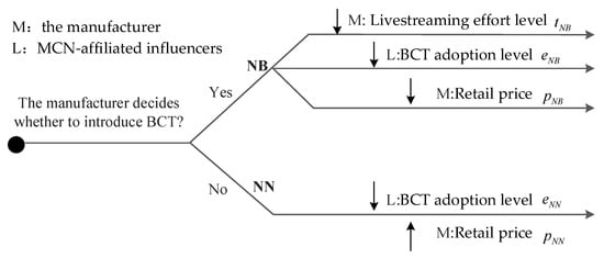
Figure 1.
The game sequence regarding whether to adopt BCT when manufacturers have unrestricted capital.
In this context, represents market potential, which reflects the exogenous underlying market size, denotes the price sensitivity of demand, indicating that for each unit increase in price, market demand decreases by units. A higher value of implies that consumers are more sensitive to price changes, leading to a faster decline in demand as prices rise. is the quality-perception coefficient; for every one-unit increase in consumers’ quality perception of the product, market demand increases by units. The larger the value , the more willing consumers are to pay for the perceived higher quality; consequently, the stronger the demand-pulling effect of the quality credibility brought by BCT. The manufacturer’s profit primarily derives from revenue generated through product sales via the livestreaming channel in collaboration with the influencer. Correspondingly, the MCN’s profit comes from the commission income based on sales, at a rate , while also bearing the effort cost incurred during livestreaming activities. Based on the above, the profit functions of the manufacturer and the MCN can be expressed as:
We employ the backward induction method to derive the equilibrium solutions for the relevant parameters. For a comprehensive view of these detailed equilibrium solutions, one can refer to Table A1 in Appendix A.
4.1.2. NB Scenario
In the NB scenario, the manufacturer chooses to adopt BCT without seeking financing, assuming that its initial capital satisfies the condition: . The sequence of decisions in this scenario (as shown in Figure 1) is characterized by a three-stage game: in Stage I, the manufacturer decides the BCT adoption level ; in Stage II, the influencer affiliated with the MCN determines their livestreaming effort level ; in Stage III, the manufacturer finally sets the product retail price . Within the framework of BCT adoption, two mechanisms come into effect: first, BCT enables quality signal transmission, allowing market participants to form a particular quality perception (upgrading from the prior expected quality perception to a determinate quality perception ); second, the application of BCT generates an independent demand expansion effect . Accordingly, the demand function in the NB scenario can be expressed as:
In these situations, the manufacturer’s and MCN’s profit functions can be expressed as follows:
We can determine the equilibrium solutions for the relevant parameters by applying the backward induction method. One can refer to Table A2 in Appendix A for a comprehensive view of these detailed equilibrium solutions. Consequently, we can reveal how BCT reshapes supply-chain participants’ strategic interactions when manufacturers have unrestricted capital, yielding Lemma 1 and Proposition 1.
Lemma 1.
Compared with the NN strategy, the impact of manufacturers adopting the NB strategy on their efforts level, product pricing, and market demand is manifested as follows: , , .
Lemma 1 indicates that, compared to the NN strategy, adopting the NB strategy leads to a significant increase in the livestreaming effort level of the MCN-affiliated influencers while enabling the manufacturer to achieve higher product pricing and greater market demand. This finding is consistent with the view of Zhang, Li, Hou, and Wang [2] that manufacturers can effectively enhance both product pricing and market demand through BCT adoption. The underlying reasons are twofold. First, the NB strategy allows the MCN and consumers to clearly and accurately perceive the manufacturer’s product quality, strengthening their trust in the manufacturer [38], thereby increasing consumers’ willingness to pay a premium for quality-assured products. Second, the introduction of BCT generates a positive market expansion effect, leading to increased market demand. Therefore, manufacturers can strengthen and enhance their competitive advantage by adopting BCT. Taking the adoption of BCT by Australia’s Penfolds as an example, the brand established a tamper-proof traceability system for its premium wines, effectively mitigating counterfeit products and strengthening consumer trust. This initiative not only reinforced its premium brand image and supported product pricing power but also facilitated successful expansion into the Chinese market.
Corollary 1.
Under the NN strategy, the impacts of the commission rate , the quality-perception coefficient , and the cost coefficient k on the manufacturer’s optimal price and market demand are as follows:
- (1)
- , , .
- (2)
- , , .
Corollary 1 shows that under the NN strategy, the manufacturer’s optimal price and market demand increase with higher commission rates and quality-perception coefficients, while the cost coefficient has no effect. Specifically, a higher commission rate leads the manufacturer to raise the retail price to offset elevated sales costs and provide influencers with more substantial incentives to enhance promotion efforts. For example, a top influencer like Li Jiaqi can stimulate purchase intention through professional live demonstrations, mitigating potential negative impacts of price increases. A higher quality-perception coefficient indicates greater consumer recognition of product quality, enabling premium pricing and further stimulating demand. It should be noted that, since BCT is not adopted in this strategy, the BCT-related cost coefficient does not affect equilibrium outcomes.
Proposition 1.
Compared with the NN strategy, when the manufacturer chooses the NB strategy, the impacts on its profit and that of the MCN are manifested as follows:
- (i)
- .
- (ii)
- When the condition is met, it occurs; when the condition occurs.
Proposition 1(i) reveals that under the NB strategy, the manufacturer’s profit is always higher than that under the NN strategy, indicating that the manufacturer achieves significantly better financial performance after adopting BCT. This finding contrasts with the view of Zhang, Li, Hou, and Wang [2], who argue that even though BCT can increase both price and demand, high-quality manufacturers may not necessarily benefit from its adoption. The key divergence stems from the fact that prior studies incorporate the information effect induced by BCT adoption—specifically, when rising information costs due to price signaling cause marginal revenue loss to exceed the benefits from basic demand expansion, BCT may fail to enhance profits for high-quality manufacturers. In contrast, our study focuses exclusively on the effect of demand expansion on BCT. Under this premise, when information cost losses are excluded, our findings demonstrate that BCT adoption in livestreaming channels is profitable for manufacturers. A case in point is a Wuyi Rock Tea producer that adopted BCT and used livestreaming to trace product origin, allowing consumers to appreciate its high quality visually. This enhanced brand trust and product value, increasing online sales from 5% to 30%.
Proposition 1(ii) indicates that when the cost of BCT adoption is low, the MCN’s profit under the NB strategy is lower than the NN strategy; conversely, when the cost is high, the MCN achieves higher profit. The underlying logic may be that lower costs encourage widespread BCT adoption among manufacturers striving for profit, intensifying competition in livestreaming channels and squeezing the MCN’s profit margin. For example, when BCT costs were low in West Lake Longjing tea, numerous tea enterprises adopted the technology, leading to a surge in traceable products. Under MCN livestreaming promotions, product homogeneity and intensified competition compressed profit margins. However, when BCT costs are high, only a few manufacturers who are committed to high-quality products adopt it. Their products gain market premiums through BCT, and the MCN can leverage this advantage by utilizing influencers’ livestreaming effectiveness to convert these premiums into channel value, thereby increasing overall profit. Therefore, when deciding whether to adopt BCT, firms should consider the adoption cost and holistically evaluate subsequent changes in market competition and their potential for profit generation within the evolving environment.
4.2. Financing Strategies for Manufacturers with Limited Capital to Adopt BCT
In this subsection, we focus on the financing strategy selection for capital-constrained manufacturers who turn to MCNs for financing when adopting BCT. Next, we will explore two financing scenarios: Scenario LB and Scenario CB.
4.2.1. LB Scenario
In the LB scenario, the MCN provides a loan to the manufacturer at an interest rate to cover the funding gap for BCT adoption. The manufacturer repays the principal plus interest at the end of the sales cycle. In practice, the LB strategy refers to an arrangement where the MCN provides a loan to the manufacturer at a pre-agreed interest rate, and the manufacturer repays the principal along with interest within a specified period. This approach constitutes a form of debt financing: the MCN earns interest income as the capital provider, while the manufacturer mitigates liquidity constraints through the injected funds. Under this scenario, the sequence of decisions is as follows (see Figure 2): First, the manufacturer adopts BCT and determines its adoption level ; then, the influencer affiliated with the MCN that cooperates with the manufacturer decides its livestreaming effort level ; finally, the manufacturer determines the retail price . Similarly, the demand function of its LSCS is the same as that in the NB scenario.
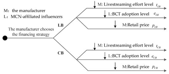
Figure 2.
The Game Sequence for Financing Strategy Selection When Manufacturers with Limited Capital Adopt BCT.
Consequently, the current-stage profit functions for the manufacturer and MCN are defined as:
The equilibrium solutions for the relevant parameters are derived through backward induction. Detailed information regarding these equilibrium solutions is in Appendix A, Table A3.
Next, we rigorously examine how pivotal parameters—BCT adoption level, influencer effort, product pricing, and market demand—shift under the LB strategy versus NB. This evaluation clarifies LB’s impact on the manufacturer’s BCT adoption decision, leading to Lemma 2.
Lemma 2.
Compared to the NB strategy, the effects of the manufacturer’s adoption of the LB strategy on its BCT adoption level, influencer livestreaming effort level, retail price, and market demand are demonstrated as follows: , , , .
Lemma 2 reveals that, compared to the NB strategy, the manufacturer’s adoption of the LB financing strategy reduces the BCT adoption level, retail price, market demand, and the influencer’s livestreaming effort. This observation aligns with the view of Marsh and Sharma [39], though it is important to note that in their study, the funding provider was a bank. Based on micro-level survey data from European small- and medium-sized enterprises, it has been found that manufacturers affected by cash flow shortages often face higher interest rates and stricter repayment conditions when obtaining loans, which further constrains their operational activities [40]. Consequently, capital-constrained manufacturers tend to adopt conservative strategies after opting for LB financing, such as reducing BCT adoption and lowering retail prices, ultimately resulting in decreased market demand and reduced livestreaming effort by influencers.
Corollary 2.
Under the NB strategy, the impacts of the commission rate , the quality-perception coefficient , and the cost coefficient k on the manufacturer’s optimal price and market demand are as follows:
- (1)
- , , .
- (2)
- , , .
Corollary 2 indicates that under the NB strategy, the manufacturer’s optimal price and market demand decrease with the commission rate and cost coefficient but increase with the quality-perception coefficient. A higher commission rate raises sales costs, leading the manufacturer to reduce prices, though demand may still decline due to lower cost-effectiveness. Similarly, increased BCT adoption costs result in price reductions and may weaken consumer trust, reducing demand. In contrast, a higher-quality-perception coefficient strengthens consumer trust through BCT traceability and authenticity, enabling higher prices and greater demand. This dual benefit is demonstrated by Feihe Milk Powder’s successful use of BCT traceability.
4.2.2. CB Scenario
Under the CB scenario, the manufacturer secures capital via an investment cost-sharing mechanism. To be precise, MCN agrees to assume a fraction of the costs associated with the manufacturer’s adoption of BCT, denoted by the investment cost-sharing ratio . It reflects the depth of cooperation between MCNs and manufacturers regarding risk and profit sharing. In contrast, the manufacturer takes on the residual costs, represented by a sharing ratio of . In practice, the CB strategy involves both parties sharing the investment costs of blockchain technology implementation according to a predetermined ratio. The MCN gains from enhanced supply chain transparency, strengthened consumer trust, and long-term collaborative benefits by absorbing part of the technological investment. Economically, this model resembles a strategic partnership mechanism based on operational synergy. The CB scenario’s decision sequence and demand function mirror the LB scenario. Likewise, the demand function for its LSCs remains consistent in the NB scenario.
The manufacturer’s and MCN’s profit functions are, thus, modeled as:
We derive the equilibrium solutions for the relevant parameters by employing the backward induction method. Detailed information regarding these equilibrium solutions is in Appendix A, Table A4.
Similarly, we analyze how CB (versus NB) alters pivotal factors, such as BCT adoption, livestreaming effort, pricing, and demand. This determines how CB affects BCT adoption decisions, and thus leads to Lemma 3.
Lemma 3.
Compared to the NB strategy, the effects of the manufacturer’s adoption of the CB strategy on its BCT adoption level, influencer livestreaming effort level, retail price, and market demand are demonstrated as follows: , , , .
Lemma 3 presents conclusions that stand in sharp contrast to those of Lemma 2. It indicates that, compared to the NB strategy, adopting the CB strategy enhances the manufacturer’s BCT adoption level, retail price, market demand, and the influencer’s livestreaming effort. This divergence can be attributed to two main reasons. On one hand, the MCN shares part of the cost of BCT adoption, effectively alleviating the manufacturer’s financial pressure—a view consistent with Dou, Wei, Sun, and Ma [5]. The reduced financial burden enables the manufacturer to increase investment in the BCT adoption level, allowing the MCN and consumers to understand product quality and enhancing consumer trust more clearly. Consequently, the manufacturer is better positioned and more confident in demonstrating the high quality of its products to consumers, which supports higher product pricing and stimulates market demand. In practice, many firms have successfully developed through cost-sharing models with manufacturers. For example, Walmart partnered with IBM to introduce BCT under a cost-sharing arrangement, achieving end-to-end transparency from raw material procurement and production to logistics and sales, thereby gaining significant consumer trust and recognition [41]. On the other hand, through livestream engagement, the manufacturer and influencer expand their follower base, enabling higher prices and greater market demand.
Corollary 3.
Under the LB strategy, the impacts of the commission rate , the quality-perception coefficient , and the cost coefficient k on the manufacturer’s optimal price and market demand are as follows:
- (1)
- , , .
- (2)
- , , .
Corollary 3 shows that under the LB strategy, the manufacturer’s optimal price and market demand decrease with the commission rate and cost coefficient but increase with the quality-perception coefficient. Specifically, a rising commission rate increases sales costs, forcing price cuts, while reduced consumer affordability further dampens demand. Additionally, the high adoption costs of BCT strain manufacturers’ finances, limiting pricing flexibility. For instance, Volvo and LG’s blockchain traceability systems, with their high costs (e.g., about USD 1.58 to store 1KB of data on Ethereum), saw reduced product demand and competitiveness. In contrast, enhanced quality perception through BCT verification and MCN financing boosts credibility, supporting higher prices and greater demand.
Moving forward, we will compare the LB and CB strategies more in-depth. This comparison assesses how different financing strategies influence the manufacturer’s decision to adopt BCT. Based on this analysis, we will subsequently formulate Lemma 4.
Lemma 4.
The differential effects of LB versus CB strategies on core variables manifest as follows: , , , .
Lemma 4 reveals that implementing the CB strategy yields higher BCT adoption, livestreaming effort, retail price, and market demand than the LB strategy. This finding aligns harmoniously with the aggregated comparative results of Lemma 2 and Lemma 3.
Corollary 4.
Under the CB strategy, the impacts of the commission rate , the quality-perception coefficient , and the cost coefficient k on the manufacturer’s optimal price and market demand are as follows:
- (1)
- , , .
- (2)
- , , .
The findings of Corollary 4 are consistent with those of Corollary 3, and the underlying logic is similar. To avoid redundancy, a detailed description is omitted here.
5. Manufacturer’s Financing Strategy Selection
In this section, we compare the profit performance of the manufacturer under three BCT adoption strategies, specifically examining the following three scenarios: NB, LB, and CB. This study provides theoretical insights to support corporate financing decisions by analyzing and comparing the manufacturer’s optimal profits across these scenarios.
Proposition 2.
Optimal manufacturer profits under NB, LB, and CB strategies compare as follows:
- (i)
- When the condition is satisfied: in the case of taking place, the outcome will occur; in the case of taking place, the outcome will happen.
- (ii)
-
Table 3. Analysis of Factors Affecting Manufacturer’s Financing Strategy Selection.
According to the “China SME Blockchain Application White Paper (2023)” and relevant industry surveys, the one-time investment cost for small- and medium-sized enterprises (SMEs) to introduce blockchain technology is usually between 200,000 and 500,000 RMB, mainly for system development, node deployment, and initial operation and maintenance. The comprehensive marginal cost of a single live broadcast (including venue, equipment, and host fees) is between 5000 and 20,000 RMB. Based on the typical profit margin structure and economies of scale in the industry, we normalized the key parameters: the potential market size is 0.4 (corresponding to a sample proportion of 1% of 120 million active users); the loan interest rate (referencing the average financing cost of SMEs in supply chain finance). To avoid distortion in numerical simulation due to excessively high influence coefficients (such as irrational surges in demand with marketing investment), we constrained all demand-related influence coefficients to be between 0 and 1. Referring to the studies of Niu, Chao, Liu, Zhang, and Luo [23] and Dong et al. [42], we assumed that and . Per the above principles, all parameter settings are shown in Table A6 in Appendix D. Based on this, we drew Figure 3, which clearly and intuitively presents the optimal financing strategy choice for the manufacturer revealed by Proposition 2.
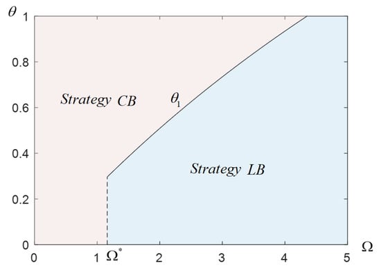
Figure 3.
Diagram of Manufacturers’ Financing Strategy Selection. Note: , , , , , , , , , .
Proposition 2 summarizes the manufacturer’s financing strategy: (i) When the manufacturer has sufficient initial capital and the MCN offers a low cost-sharing ratio, the LB strategy is preferred; otherwise, the CB strategy is chosen. (ii) The CB strategy is superior when initial capital is limited. This conclusion contrasts with Niu, Chao, Liu, Zhang, and Luo [23], who argued that the CB strategy is beneficial when initial capital is sufficient and the cost-sharing ratio is low. The difference arises from our inclusion of multidimensional factors such as the initial BCT funding gap, financing cost dynamics, and demand enhancement effects. With sufficient initial capital, a smaller funding gap, and lower financing costs, the LB strategy is preferable under a low MCN cost-sharing ratio. A higher ratio favors the CB strategy. The case of Kweichow Moutai supports these findings: initially, sufficient capital and low adoption costs made the LB strategy feasible. As BCT’s value became apparent, MCNs (e.g., e-commerce platforms) shared costs to benefit from traceability, leading to a shift toward the CB strategy. In this arrangement, the MCN bears a larger share of the adoption cost, reducing the manufacturer’s financial burden. At the same time, the demand enhancement effect—such as increased prices and sales in livestreaming—becomes dominant. When the manufacturer’s initial capital is limited, the CB strategy proves more advantageous due to a larger BCT funding gap and higher financing costs. With fixed repayments and interest obligations, the LB strategy could exacerbate financial strain and increase bankruptcy risks [43]. For example, the Dr. Schneider Group faced high-interest loans and rigid repayment terms, resulting in operational failure and bankruptcy due to poor debt management. Thus, manufacturers should holistically evaluate their initial capital and the MCN’s investment cost-sharing ratio, while considering financing risks, to select the optimal strategy.
6. Analysis of MCN’s Profit and Loss
In this section, we investigate the impact of the manufacturer’s financing strategy selection on the profit of the MCN to examine the MCN’s cooperative inclination.
Proposition 3.
The impact of manufacturers’ financing strategy selections on MCN’s profit and loss is manifested in the following aspects:
- (i)
- When the condition is satisfied, the outcome will occur.
- (ii)
- When the condition is satisfied: in the case of taking place, the outcome will occur; in the case of taking place, the outcome will happen (Figure 4, Table 4).
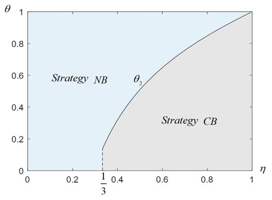 Figure 4. Diagram of Profit and Loss Variations for MCNs. Note: , , , , , , , , , .
Table 4. Analysis of Factors Affecting MCN Profit and Loss.
Figure 4. Diagram of Profit and Loss Variations for MCNs. Note: , , , , , , , , , .
Table 4. Analysis of Factors Affecting MCN Profit and Loss.
Proposition 3 examines how manufacturers’ financing choices affect MCN profit. Specifically: (i) Under low commission rates, MCNs prefer the NB strategy; (ii) Under high commission rates, MCNs choose the CB strategy when their investment cost-sharing ratio is low; otherwise, they still prefer NB. This contrasts with Ma, Dai, and Li [17] and Chang, Li, Wang, and Wang [25]. The former suggested that high commissions make MCNs more willing to offer loans, while the latter argued that high commissions coupled with financing may create misaligned incentives. The difference arises because our model incorporates loan provision and investment cost-sharing, while prior work focused only on financing. Two underlying mechanisms explain these results. Under low commission rates, both the LB and CB strategies further compress MCN profit. In the case of LB financing, additional costs and risks reduce the effort level of livestreaming and diminish fan engagement. In contrast, under CB, the increase in revenue fails to cover the associated financing costs. By contrast, a low investment cost-sharing ratio under high commission rates makes the CB strategy more advantageous, as MCNs retain higher per-unit revenue. At the same time, the manufacturer bears a greater share of the costs. This leads to improved overall returns and encourages better livestream performance. However, if the investment cost-sharing ratio is high, MCNs face substantial cost burdens even when high commission rates, making the NB strategy a safer alternative. For example, despite multiple financings during 2023–2024, Lily & Beauty saw profit decline under low commission rates due to rising operational costs. Thus, MCNs must carefully weigh commission rates and cost-sharing ratios when selecting collaboration modes with manufacturers.
7. Conclusions
With the rapid adoption of BCT, many manufacturers are leveraging it to enhance the traceability and transparency of product quality. However, when introducing BCT into LSCs, manufacturers may encounter financial constraints due to the high costs involved. To address this challenge, we develop four strategies based on whether the manufacturer adopts BCT and the type of financing used, providing a comprehensive analysis of the manufacturer’s financing strategy choices in the process of BCT adoption. Furthermore, we examine how the manufacturer’s financing strategy affects the profit of the MCN to evaluate the MCN’s willingness to cooperate, deriving several essential findings and managerial insights.
7.1. Main Findings
The main findings are as follows. First, for manufacturers without financial constraints, BCT adoption consistently yields positive effects: it raises influencers’ effort levels in LSCs, which in turn increases retail pricing, expands market demand, and ultimately enhances profits through an “efficiency–price–demand” value chain. However, capital-constrained manufacturers must seek financing from MCNs due to high adoption costs. Specifically, when initial capital is sufficient and the MCN’s investment cost-sharing ratio is low, the manufacturer chooses the LB strategy. Interestingly, the CB strategy is preferred when initial capital is low, or even if sufficient, but the MCN’s investment cost-sharing ratio is high.
Second, the CB and LB strategies lead to notable differences in retail pricing and market performance compared to the NB strategy. Under the LB strategy, both the retail price and market demand are significantly lower. In contrast, the CB strategy results in substantially higher pricing and improved market outcomes. Notably, both price and demand under CB exceed those under LB, which is consistent with earlier findings. The key reason is that, unlike LB, the CB strategy imposes no fixed repayment or interest obligations, reducing the manufacturer’s financial pressure. In addition, participation in collaborative efforts with influencers encourages the manufacturer to improve product quality and expand market reach, driving simultaneous growth in both price and demand.
Finally, the manufacturer’s financing strategy affects the MCN’s profit and loss through the investment cost-sharing ratio and the commission rate. When the commission rate is low, or high but paired with a high-investment cost-sharing ratio, the financing strategy erodes the MCN’s profit beyond its risk tolerance, leading it to prefer the NB strategy. When the commission rate is high and the investment cost-sharing ratio is low, the effects diverge: the CB strategy creates synergistic benefits with limited cost burden. In contrast, the LB strategy causes budget crowding-out in the channel due to combined interest and commission costs. Thus, the MCN tends to choose CB under such conditions. Consequently, MCNs should closely monitor the commission rate and investment cost-sharing ratio to achieve a Pareto-optimal balance between technology investment and profit distribution.
7.2. Practical Implications for Management
Practical management implications are outlined as follows. First, manufacturers should recognize that adopting BCT consistently delivers multiple benefits when no financial constraints exist. It enables higher pricing and enhanced market performance, significantly increasing profit levels. For instance, a Wuyi Rock Tea producer adopted BCT with livestreaming traceability, which raised online sales from 5% to 30%. For capital-constrained manufacturers seeking quality improvement through BCT, obtaining financing from MCNs offers a viable pathway. However, real-world cases like the Dr. Schneider Group, an automotive parts manufacturer that experienced capital chain breakdowns due to poorly managed loans, underscore the need to thoroughly evaluate initial capital and financing risks before selecting the optimal method.
Second, from the MCN’s perspective as a capital provider, it should closely monitor how the manufacturer’s financing strategy affects its profit to minimize risk and ensure profitability. For example, Lily & Beauty conducted multiple financings in a low-commission environment. Still, she saw profit decline due to rising R&D and marketing costs, illustrating that MCNs must balance risk and return while strengthening risk awareness in such contexts. Furthermore, our findings show that when the commission rate is low or high but paired with a high cost-sharing ratio, the MCN lacks motivation to provide financial support, as either financing strategy may erode its profit. Conversely, when the commission rate is high and the cost-sharing ratio is relatively low, the MCN should consider cooperating through the CB strategy, which can meet the manufacturer’s funding needs while effectively maximizing the MCN’s profit. Therefore, MCNs should pay close attention to the manufacturer’s financing strategy, particularly the effects of commission rate and investment cost-sharing ratio.
Third, from the consumer’s perspective, BCT adoption enhances precise product awareness, safeguards consumer interests, and significantly improves transparency and trust in consumption. By using BCT, consumers can trace comprehensive key information such as production origin, circulation path, and quality inspections, ensuring the authenticity and reliability of purchased goods. For instance, Walmart employs BCT to track end-to-end food products like leafy greens. By scanning a QR code, consumers gain immediate access to complete circulation data from farm to store and detailed step-by-step information, allowing them to make more informed and confident purchasing decisions.
Fourth, when making supply chain financing decisions, enterprises should select between the LB or CB strategy according to their capital availability and their partners’ willingness to share costs. The LB strategy is suitable when the firm has sufficient funds and the partner offers a low cost-sharing ratio. For example, Kuaishou-supported brands used loans to expand operations when subsidies were limited. The CB strategy is preferable when the partner bears a high-cost ratio or the firm is capital-constrained, as Yaowang Network’s joint brand investments demonstrate. Companies in sectors such as food and agriculture can also adopt BCT to enhance supply chain transparency and traceability. For instance, Kerchin Cattle Industry strengthened consumer trust through full-process data management, and influencer collaborations like Xin Youzhi’s promotion of traceable Wuchang rice boosted sales and brand value.
7.3. Limitations and Directions for Future Work
Our study has several limitations that also suggest directions for future research. First, we conducted a simulation analysis through theoretical modeling. In the future, we can further evaluate whether the simulation results align with real-world corporate behaviors by empirically validating case studies on significant platforms such as TikTok or RED. Second, the current model incorporates only two financing strategies; future work could examine hybrid approaches that combine LB and CB strategies and platform financing elements to evaluate their impact on manufacturer decisions. Furthermore, incorporating a demand function derived from consumer utility theory, such as a Logit model, would help better capture saturation effects and diminishing marginal utility, thus improving the micro-foundations and behavioral realism of the demand model. Finally, future studies could include additional factors such as risk attitudes of supply chain members toward BCT, network effects, and technical limitations to enable a more comprehensive understanding of BCT adoption and financing decisions.
Author Contributions
Conceptualization, S.F. and J.L. (Jiqiong Liu); methodology, S.F.; formal analysis, J.L. (Jing Liu); data curation, J.L. (Jing Liu); writing—original draft, J.L. (Jing Liu); writing—review & editing, S.F. and J.L. (Jiqiong Liu); supervision, J.L. (Jiqiong Liu); funding acquisition, J.L. (Jiqiong Liu). All authors have read and agreed to the published version of the manuscript.
Funding
This research was supported by the National Natural Science Foundation of China [grant numbers 72171067 and 72401002], the University Natural Science Research Project of Anhui Province [grant numbers 2022AH051323], the Excellent Young Talents Fund Program of Higher Education Institutions of Anhui Province [grant number JNFX2024036], the Doctoral Foundation of Fuyang Normal University [grant numbers 2021KYQD0007 and 2021KYQD0015], and the Graduate Education Quality Engineering Project of Anhui Province under Grant 2024cxcysj164 and Grant 2024cxcysj165. These funding sources do not lead to any conflicts of interest with the publication of this paper.
Data Availability Statement
The original contributions presented in this study are included in the article. Further inquiries can be directed to the corresponding author.
Conflicts of Interest
The authors declare no conflicts of interest.
Abbreviations
The following abbreviations are used in this manuscript:
| LSCs | live-streaming supply chains |
| BCT | blockchain technology |
| MCNs | Multi-Channel Networks |
| SCF | Supply chain financing |
Appendix A. Equilibrium Solutions and Thresholds
Table A1.
Equilibrium Solutions under Scenario NN.
Table A1.
Equilibrium Solutions under Scenario NN.
Table A2.
Equilibrium Solutions under Scenario NB.
Table A2.
Equilibrium Solutions under Scenario NB.
Table A3.
Equilibrium Solutions under Scenario LB.
Table A3.
Equilibrium Solutions under Scenario LB.
Table A4.
Equilibrium Solutions under Scenario CB.
Table A4.
Equilibrium Solutions under Scenario CB.
Table A5.
Relevant Thresholds.
Table A5.
Relevant Thresholds.
Appendix B. Proof of Equilibrium Solutions
Appendix B.1. NN Strategy
We employ backward induction to derive the equilibrium outcomes for each scenario:
Substituting into Equations (2) and (3), we obtain:
Taking the first-order and second-order partial derivatives of Equation (A1) yields:
Since the second-order derivative is less than 0, the function has a unique maximum (which is also the global maximum in this case). Therefore, by setting the first-order derivative equal to 0, we obtain:
Substitute the obtained solution into Equation (A2), then take the first-order partial derivative concerning the relevant variable(s) and simplify the expression:
Since the second-order derivative is less than zero, the function has a unique maximum (the global maximum in this case). Therefore, by setting the first-order derivative equal to zero, we obtain:
This represents the Unique point of maximum (i.e., the global maximum).
Substituting Equation (A8) into Equation (A5), we obtain:
Substituting these values into the aforementioned optimal results and simplifying, we obtain the equilibrium outcomes presented in Table A1.
Appendix B.2. NB Strategy
Similarly, we employ backward induction to derive the equilibrium outcomes for each model:
Substituting into Equations (5) and (6), we obtain:
Taking the first-order and second-order partial derivatives of Equation (A10) yields:
Since the second-order derivative is less than zero, the function has a unique maximum (which is the global maximum), so setting the first-order derivative to zero yields:
Substitute the solved expression into Equation (A11), then compute its first-order partial derivatives and simplify the results:
Since the second-order derivative is less than zero, the function has a unique maximum (which serves as the global maximum in this context). Therefore, by setting the first-order derivative equal to zero, we obtain:
It is readily apparent that this represents the sole point of local maximality, which consequently corresponds to the global maximum.
Substituting Equation (A17) into Equation (A14) yields:
Similarly, by taking the first-order and second-order partial derivatives of Equation (A10), we obtain:
Since the second-order derivative is less than zero, the function attains a unique local maximum, the global maximum under the given conditions. Setting the first-order derivative(s) equal to zero yields:
Substituting Equation (A21) into Equations (A17) and (A18), we obtain:
Subsequently, substituting these derived expressions into the aforementioned optimal conditions and simplifying the equations, we obtain the equilibrium results in Table A2.
Appendix B.3. LB Strategy
This financing method involves an MCN providing a loan to the manufacturer at a set interest rate to support BCT adoption, with principal repayment and interest from the manufacturer’s product sales revenue. Its core economic logic lies in aligning interests via a credit relationship: the MCN gains interest income and strengthens collaboration. At the same time, the manufacturer reduces financial pressure and boosts sales through livestreaming. This approach supports small and medium-sized enterprises while also requiring careful management of financial risks.
Similarly, substituting into Equations (8) and (9) yields:
By taking the first-order and second-order partial derivatives of Equation (A24) concerning the relevant variables, we obtain:
Since the second-order derivative is less than zero, the function has a unique maximum (which is the global maximum), so setting the first-order derivative to zero yields:
Substitute the solved expression into Equation (A25), then compute its first-order partial derivatives and simplify the results:
Since the second-order derivative is less than zero, the function attains a unique local maximum, the global maximum under the given conditions. Setting the first-order derivative(s) equal to zero yields:
It is readily apparent that this represents the sole point of local maximality, which consequently corresponds to the global maximum.
Substituting Equation (A31) into Equation (A28) yields:
Similarly, by calculating the first-order and second-order partial derivatives of Equation (A24) concerning the relevant variables, we obtain:
Since the second-order derivative is less than zero, the function has a unique maximum (which is the global maximum), so setting the first-order derivative to zero yields:
Substituting Equation (A35) into Equations (A31) and (A32) yields:
Subsequently, substituting these derived expressions into the aforementioned optimal conditions and simplifying the equations, we obtain the equilibrium results presented in Table A3.
Appendix B.4. CB Strategy
This financing model describes an arrangement where the MCN shares part of the manufacturer’s costs for adopting BCT in return for long-term benefits, such as improved traceability. The core economic mechanism is based on a shared risk–return structure that enhances sales conversion rates and brand loyalty through collaboration. From a policy standpoint, defining regulatory compliance for such partnerships is critical. At the same time, tax incentives should be considered to encourage MCN participation in real-economy innovation, helping foster deeper integration of technology and industry.
Similarly, substituting into Equations (11) and (12) yields:
By taking the first-order and second-order partial derivatives of Equation (A38) concerning the relevant variables, we obtain:
Since the second-order derivative is less than zero, the function has a unique maximum (which is the global maximum), so setting the first-order derivative to zero yields:
Substitute the solved expression into Equation (A39), then compute its first-order partial derivatives and simplify the results:
Since the second-order derivative is less than zero, the function attains a unique local maximum, the global maximum under the given conditions. Setting the first-order derivative(s) equal to zero yields:
It is readily apparent that this represents the sole point of local maximality, which consequently corresponds to the global maximum.
Substituting Equation (A45) into Equation (A42) yields:
Similarly, by calculating the first-order and second-order partial derivatives of Equation (A38) concerning the relevant variables, we obtain:
Since the second-order derivative is less than zero, the function has a unique maximum (which is the global maximum), so setting the first-order derivative to zero yields:
Substituting Equation (A49) into Equations (A45) and (A46) yields:
Subsequently, substituting these derived expressions into the aforementioned optimal conditions and simplifying the equations, we obtain the equilibrium results presented in Table A4.
Appendix C. Proofs of Lemmas, Propositions, and Corollaries
Appendix C.1. Proof of Lemma 1
Proof of Lemma 1.
, , . Where and hold. Therefore, .
, , . Where and hold. Therefore, .
, . Consequently, we obtain . Hence, holds. This completes the proof of Lemma 1. □
Appendix C.2. Proof of Lemma 2
Proof of Lemma 2.
, , . Where and hold. Therefore, we obtain .
, , . Where: . Therefore, we obtain .
, . Where and hold. Therefore, we obtain .
. Similarly, we obtain . Therefore, .This completes the proof of Lemma 2. □
Appendix C.3. Proof of Lemma 3
Proof of Lemma 3.
, , . Where: and hold. Therefore, we obtain .
, , . Where and hold. Therefore, we obtain .
, , . Where and hold. Therefore, we obtain .
Similarly, . This completes the proof of Lemma 3. □
Appendix C.4. Proof of Lemma 4
Proof of Lemma 4.
From the above, we obtain . Where and hold. Therefore, we obtain .
. Where we hold. Therefore, we obtain .
. Where we hold. Consequently, we obtain .
Similarly, . This completes the proof of Lemma 4. □
Appendix C.5. Proof of Proposition 1
Proof of Proposition 1.
, , . Where and hold. It follows that it is a linear function of . Given: and . Therefore, we can conclude that is a linear function with a positive slope and an intercept. Consequently, is thus established. Therefore, .
, , . Where and hold.
It follows that is a univariate quadratic function of . Given: , , . Since it holds admits real solutions. Upon verification, we conclude is a convex function with two distinct real roots (denoting the positive root as ). Therefore: When holds, is satisfied, and, thus, follows; when holds, is satisfied; thus, follows.
In summary: When holds, is established; when holds, is established. This completes the proof of Proposition 1. □
Appendix C.6. Proof of Proposition 2
Proof of Proposition 2.
Compared with the NB strategy, when the manufacturer adopts the LB strategy, the profit comparison is as follows:
,
. Where and hold. We define , and thus, when occurs, is satisfied; when occurs, is satisfied.
Profit comparison between the manufacturer’s choice of CB strategy versus NB strategy:
, , . Where and hold. Therefore, we can derive that .
Profit comparison between the manufacturer’s adoption of the LB and CB strategies:
Similarly, . Where, and hold.
.
Consequently, we establish that is a linear function with a negative slope and a positive y-intercept, intersecting the x-axis at point (). This leads to the following conclusions: when holds, is satisfied, implying ;
When it occurs, it is validated, resulting in .
In conclusion, we establish the following results under the condition : implies ; implies . Furthermore, is universal when is satisfied.
This completes the proof of Proposition 2. □
Appendix C.7. Proof of Proposition 3
Proof of Proposition 3.
Compared with the NB strategy, when MCN adopts the LB strategy, the profit comparison is as follows: similarly, . Where , and hold, respectively. Consequently, we obtain .
Profit comparison between MCN’s choice of CB strategy versus NB strategy:
Similarly, , where and hold. Moreover, ,
.
Where holds.
Consequently, when the condition holds, we obtain , which implies and . This establishes a concave function with two real roots: a zero root and a positive root, denoted as . Further implications: When is satisfied, holds, yielding ; when occurs, is validated, resulting in .
Under the condition , we derive , which implies . Consequently, is established as a concave function with two real roots: zero and negative. This leads to the conclusion that holds, thereby yielding .
In summary, the following results are obtained:
When , the condition is satisfied, and is validated;
For all , holds universally.
Profit comparison between MCN’s adoption of the LB strategy and CB strategy:
. From the preceding analysis, we establish that holds. This leads to the derivation of , which subsequently implies .
In summary, the following results are obtained:
holds universally under a condition ; when is satisfied, if occurs, then follows; If holds, then is validated.
This completes the proof of Proposition 3. □
Appendix C.8. Proof of Corollary 1
Proof of Corollary 1.
- (1)
- , , .
- (2)
- , , .
□
Appendix C.9. Proof of Corollary 2
Proof of Corollary 2.
- (1)
- , , .
- (2)
- , , .
□
Appendix C.10. Proof of Corollary 3
Proof of Corollary 3.
- (1)
- , , .
- (2)
- , , .
□
Appendix C.11. Proof of Corollary 4
Proof of Corollary 4.
- (1)
- , , ,
- (2)
- , , .
□
Appendix D. Parameter Rationality Explanation
Table A6.
Parameter Rationality Explanation.
Table A6.
Parameter Rationality Explanation.
| Parameters | Definition | Bound | Origin | Rationale |
|---|---|---|---|---|
| Effort effectiveness coefficient of influencer livestreaming | It is assumed that the real-time interactivity of influencers affiliated with the MCN exerts a relatively strong direct effect on stimulating demand. | Refer to Liu et al. [44] | ||
| Perceived quality coefficient | Constant marginal effect | Refer to Niu, Chao, Liu, Zhang, and Luo [23] | ||
| The livestreaming effort level of influencers | The law of increasing marginal cost | Refer to He et al. [45] | ||
| Market potential | The active user base of the platform (for example, Douyin’s clothing market has approximately 120 million users) | Refer to Niu et al. [46] | ||
| Price sensitivity of demand | Price elasticity of demand | Refer to Dong, Huang, and Fang [42] | ||
| Effect of the coefficient of BCT adoption level on demand enhancement | Information asymmetry and signaling theory | Refer to Cheng et al. [47] | ||
| Interest rate | The average financing cost of SMEs in supply chain finance | Refer to Yi et al. [48] | ||
| Commission rate | The actual commission rate range of the platform (for example, the commission rate of Douyin is usually less 50%) | Refer to Niu et al. [49] | ||
| BCT adoption cost coefficient | Adopting it all at once, and the fact that SMEs are capital-constrained. | Refer to Jiang, Yao, Li, and Wei [31] | ||
| The follower level of MCN-affiliated influencers | Follower base and scale effects | Refer to Da, Gou, and Liang [36] |
References
- Wang, X.; Han, X.; Chen, Y. Optimal manufacturer strategy for live-stream selling and product quality. Electron. Commer. Res. Appl. 2024, 64, 101372–101384. [Google Scholar] [CrossRef]
- Zhang, Q.; Li, Y.; Hou, P.; Wang, J. Price signal or blockchain technology? Quality information disclosure in dual-channel supply chains. Eur. J. Oper. Res. 2024, 316, 126–137. [Google Scholar] [CrossRef]
- Wang, J.; Zhang, Q.; Hou, P. Combating Deceptive Counterfeits With Blockchain Technology Under Asymmetric Information. IEEE Trans. Eng. Manag. 2024, 71, 3951–3963. [Google Scholar] [CrossRef]
- Zhu, S.; Li, J.; Wang, S.; Xia, Y.; Wang, Y. The role of blockchain technology in the dual-channel supply chain dominated by a brand owner. Int. J. Prod. Econ. 2023, 258, 108791–108806. [Google Scholar] [CrossRef]
- Dou, G.; Wei, K.; Sun, T.; Ma, L. Blockchain technology adoption in a supply chain: Channel leaderships and environmental implications. Transp. Res. Part E Logist. Transp. Rev. 2024, 192, 103788–103810. [Google Scholar] [CrossRef]
- Fang, C.; Chi, M.; Fan, S.; Choi, T.-M. Who should invest in blockchain technology under different pricing models in supply chains? Eur. J. Oper. Res. 2024, 319, 777–792. [Google Scholar] [CrossRef]
- Liu, X.; Zhou, Z.; Hu, M.; Zhong, F. How retailers can gain more profitability driven by digital technology: Live streaming promotion and blockchain technology traceability? Electron. Commer. Res. Appl. 2024, 68, 101445–101464. [Google Scholar] [CrossRef]
- Guo, P.; Feng, G.; Wang, K.; Zhou, X.; Liu, Q. Analysis of blockchain technology implementing and financing provision strategies in contract farming supply chains. Transp. Res. Part E Logist. Transp. Rev. 2025, 203, 104385–104408. [Google Scholar] [CrossRef]
- Caliskan, F.; Idug, Y.; Gligor, D.; Hong, S.-J. Blockchain technology for building buyer-supplier trust and transparency in supply chains: An experimental study on P2P online marketplace vendors. Ind. Mark. Manag. 2025, 124, 239–253. [Google Scholar] [CrossRef]
- Klöckner, M.; Schmidt, C.G.; Wagner, S.M. When Blockchain Creates Shareholder Value: Empirical Evidence from International Firm Announcements. Prod. Oper. Manag. 2022, 31, 46–64. [Google Scholar] [CrossRef]
- Xu, X.; Chen, X.; Cheng, T.C.E.; Choi, T.-M.; Yang, Y. Should blockchain be used to eliminate greenwashing for green and live-streaming platform operations under carbon trading systems? Eur. J. Oper. Res. 2025, 324, 1017–1034. [Google Scholar] [CrossRef]
- Dai, B.; Nu, Y.; Xie, X.; Li, J. Interactions of traceability and reliability optimization in a competitive supply chain with product recall. Eur. J. Oper. Res. 2021, 290, 116–131. [Google Scholar] [CrossRef]
- Wu, C.; Xu, C.; Zhao, Q.; Zhu, J. Research on financing strategy under the integration of green supply chain and blockchain technology. Comput. Ind. Eng. 2023, 184, 109598–109617. [Google Scholar] [CrossRef]
- Mandal, P.; Basu, P.; Choi, T.-M.; Rath, S.B. Platform financing vs. bank financing: Strategic choice of financing mode under seller competition. Eur. J. Oper. Res. 2024, 315, 130–146. [Google Scholar] [CrossRef]
- Qin, J.; Fu, H.; Wang, Z.; Xia, L. Financing and carbon emission reduction strategies of capital-constrained manufacturers in E-commerce supply chains. Int. J. Prod. Econ. 2021, 241, 108271–108291. [Google Scholar] [CrossRef]
- Lu, W.; Ji, X.; Wu, J. Retailer’s information sharing and manufacturer’s channel expansion in the live-streaming E-commerce era. Eur. J. Oper. Res. 2025, 320, 527–543. [Google Scholar] [CrossRef]
- Ma, C.; Dai, Y.; Li, Z. Financing format selection for electronic business platforms with a capital-constrained e-tailer. Transp. Res. Part E Logist. Transp. Rev. 2022, 162, 102720–102746. [Google Scholar] [CrossRef]
- Xie, X.; Xu, X.; Zhang, C.; Zhang, F. Enhancing a triple capital-constrained supply chain performance: Alliance financing, profit distribution, and information structure. Int. J. Prod. Econ. 2025, 281, 109515–109542. [Google Scholar] [CrossRef]
- Li, Y.; Ou, J.; Gu, C. Buyer guarantee and bailout in supplier finance with bankruptcy cost. Eur. J. Oper. Res. 2023, 305, 287–299. [Google Scholar] [CrossRef]
- Sun, S.; Hua, S.; Liu, Z. Navigating default risk in supply chain finance: Guidelines based on trade credit and equity vendor financing. Transp. Res. Part E Logist. Transp. Rev. 2024, 182, 103410–103425. [Google Scholar] [CrossRef]
- Tang, T.; Xu, H.; Chen, K.; Zhang, Z. Optimal financing and sales channel strategies for a capital-constrained supply chain with different risk preferences. Comput. Ind. Eng. 2024, 187, 109813–109829. [Google Scholar] [CrossRef]
- Cao, C.; He, Y.; Liu, Y.; Huang, H.; Zhang, F. Blockchain technology adoption mechanism for semiconductor chip supply chains considering information disclosure under cost-sharing contract. Int. J. Prod. Econ. 2025, 282, 109496–109519. [Google Scholar] [CrossRef]
- Niu, W.; Chao, X.; Liu, L.; Zhang, L.; Luo, M. Financial support to a supplier for quality improvement in a dual-channel supply chain. Comput. Ind. Eng. 2024, 189, 109975–109988. [Google Scholar] [CrossRef]
- Shen, J.; Yan, H.; Sheng, L.; Zhang, B.; Shi, Y.; Shen, S. Pricing decision in an uncertain green product supply chain under cost sharing contract. Expert Syst. Appl. 2024, 250, 123899–123912. [Google Scholar] [CrossRef]
- Chang, S.; Li, A.; Wang, X.; Wang, X. Joint optimization of e-commerce supply chain financing strategy and channel contract. Eur. J. Oper. Res. 2022, 303, 908–927. [Google Scholar] [CrossRef]
- Gao, Y.; Gao, H.; Xiao, H.; Yao, F. Vaccine supply chain coordination using blockchain and artificial intelligence technologies. Comput. Ind. Eng. 2023, 175, 108885–108909. [Google Scholar] [CrossRef] [PubMed]
- Flovik, S.; Moudnib, R.A.R.; Vassilakopoulou, P. Determinants of Blockchain Technology Introduction in Organizations: An Empirical Study among Experienced Practitioners. Procedia Comput. Sci. 2021, 181, 664–670. [Google Scholar] [CrossRef]
- Jasrotia, S.S.; Rai, S.S.; Rai, S.; Giri, S. Stage-wise green supply chain management and environmental performance: Impact of blockchain technology. Int. J. Inf. Manag. Data Insights 2024, 4, 100241–100251. [Google Scholar] [CrossRef]
- Li, Z.; Xu, Z. Digital technology and innovation:The impact of blockchain application on enterprise innovation. Technovation 2025, 139, 103136–103148. [Google Scholar] [CrossRef]
- Cui, Y.; Gaur, V.; Liu, J. Supply Chain Transparency and Blockchain Design. Manag. Sci. 2023, 70, 3245–3263. [Google Scholar] [CrossRef]
- Jiang, L.; Yao, A.; Li, W.; Wei, Q. Blockchain technology empowers the cross-border dual-channel supply chain: Introduction strategy, tax differences, optimal decisions. Comput. Ind. Eng. 2024, 195, 110431–110458. [Google Scholar] [CrossRef]
- Xu, X.; Chen, X.; Hou, J.; Cheng, T.C.E.; Yu, Y.; Zhou, L. Should live streaming be adopted for agricultural supply chain considering platform’s quality improvement and blockchain support? Transp. Res. Part E Logist. Transp. Rev. 2025, 195, 103950–103985. [Google Scholar] [CrossRef]
- Iyengar, G.; Saleh, F.; Sethuraman, J.; Wang, W. Blockchain Adoption in a Supply Chain with Manufacturer Market Power. Manag. Sci. 2023, 70, 6158–6178. [Google Scholar] [CrossRef]
- Liu, X.; Zhou, Z.; Zhong, F.; Hu, M. Resolving the information reliability issue in live streaming through blockchain adoption. Transp. Res. Part E Logist. Transp. Rev. 2024, 189, 103652–103679. [Google Scholar] [CrossRef]
- Jiang, R.; Kang, Y.; Liu, Y.; Liang, Z.; Duan, Y.; Sun, Y.; Liu, J. A trust transitivity model of small and medium-sized manufacturing enterprises under blockchain-based supply chain finance. Int. J. Prod. Econ. 2022, 247, 108469–108490. [Google Scholar] [CrossRef]
- Da, Y.; Gou, Q.; Liang, C. Will self-gifting of streamers hurt unions? Analyzing the union’s compensation mechanism for a live streaming supply chain. Transp. Res. Part E Logist. Transp. Rev. 2023, 177, 103230–103252. [Google Scholar] [CrossRef]
- Liu, J.; Yuan, R.; Feng, S.; Wang, G. Quality-differentiated distribution strategies between live streaming and online channels. J. Retail. Consum. Serv. 2025, 82, 104056–104077. [Google Scholar] [CrossRef]
- Le, M.T.H. Fostering product quality and Brand Trust by QR code traceability and customer reviews: The moderating role of brand reputation in Blockchain. J. High Technol. Manag. Res. 2024, 35, 100492–100502. [Google Scholar] [CrossRef]
- Marsh, W.B.; Sharma, P. Loan guarantees in a crisis: An antidote to a credit crunch? J. Financ. Stab. 2024, 72, 101244–101263. [Google Scholar] [CrossRef]
- Kaya, O. The impact of late payments on SMEs’ access to finance: Evidence from credit rationing and loan terms. Econ. Model. 2024, 141, 106896–106908. [Google Scholar] [CrossRef]
- Bae, S.H.; Saberi, S.; Kouhizadeh, M.; Sarkis, J. Evaluating blockchain technology adoption in multi-tier supply chains from an institutional entrepreneurship theory perspective. Transp. Res. Part C Emerg. Technol. 2024, 160, 104510–104530. [Google Scholar] [CrossRef]
- Dong, C.; Huang, Q.; Fang, D. Channel selection and pricing strategy with supply chain finance and blockchain. Int. J. Prod. Econ. 2023, 265, 109006–109020. [Google Scholar] [CrossRef]
- Lin, Q.; Shan, Z.; Fu, W.; Lin, X. Interplay between the agriculture firm’s guarantee strategy and the e-commerce platform’s loan strategy with risk averse farmers. Omega 2024, 127, 103108–103122. [Google Scholar] [CrossRef]
- Liu, Z.; Chen, H.; Zhang, X.; Gajpal, Y.; Zhang, Z. Optimal channel strategy for an e-seller: Whether and when to introduce live streaming? Electron. Commer. Res. Appl. 2024, 63, 101348–101371. [Google Scholar] [CrossRef]
- He, P.; Shang, Q.; Pedrycz, W.; Chen, Z.-S. Short video creation and traffic investment decision in social e-commerce platforms. Omega 2024, 128, 103129–103144. [Google Scholar] [CrossRef]
- Niu, B.; Dong, J.; Yu, X.; Wang, Y. Online quality endorsement to improve consumer trust: Blockchain or self-hosted livestream? Eur. J. Oper. Res. 2025; in press. [Google Scholar] [CrossRef]
- Cheng, S.; Li, D.; Liu, T. Pricing and green investment of technology-differentiated manufacturers under blockchain technology. Comput. Ind. Eng. 2025, 208, 111418–111435. [Google Scholar] [CrossRef]
- Yi, Z.; Chen, Y.; Luo, S.; Huang, H. Agricultural supply chain finance considering interest or direct subsidy by government. Transp. Res. Part E Logist. Transp. Rev. 2025, 195, 103992–104007. [Google Scholar] [CrossRef]
- Niu, B.; Chen, Y.; Zhang, J.; Chen, K.; Jin, Y. Brands’ Livestream Selling with Influencers’ Converting Fans into Consumers. Omega 2025, 131, 103195–103206. [Google Scholar] [CrossRef]
Disclaimer/Publisher’s Note: The statements, opinions and data contained in all publications are solely those of the individual author(s) and contributor(s) and not of MDPI and/or the editor(s). MDPI and/or the editor(s) disclaim responsibility for any injury to people or property resulting from any ideas, methods, instructions or products referred to in the content. |
© 2025 by the authors. Licensee MDPI, Basel, Switzerland. This article is an open access article distributed under the terms and conditions of the Creative Commons Attribution (CC BY) license (https://creativecommons.org/licenses/by/4.0/).