Abstract
Feature map pooling in convolutional neural networks (CNNs) serves the dual purpose of reducing spatial dimensions and enhancing feature invariance. Current pooling approaches face a fundamental trade-off: deterministic methods (e.g., MaxPool and AvgPool) lack regularization benefits, while stochastic approaches introduce beneficial randomness but can suffer from sampling biases and may require careful hyperparameter tuning (e.g., S3Pool). To address these limitations, this paper introduces LDS3Pool, a novel pooling method that leverages low-discrepancy sequences (LDSs) for quasi-random spatial sampling. LDS3Pool first linearizes 2D feature maps to 1D sequences using Hilbert space-filling curves to preserve spatial locality, then applies LDS-based sampling to achieve quasi-random downsampling with mathematical guarantees of uniform coverage. This framework provides the regularization benefits of randomness while maintaining comprehensive feature representation, without requiring sensitive hyperparameter tuning. Extensive experiments demonstrate that LDS3Pool consistently outperforms baseline methods across multiple datasets and a range of architectures, from classic models like VGG11 to modern networks like ResNet18, achieving significant accuracy gains with moderate computational overhead. The method’s empirical success is supported by a rigorous theoretical analysis, including a quantitative evaluation of the Hilbert curve’s superior, size-independent locality preservation. In summary, LDS3Pool represents a theoretically sound and empirically effective pooling method that enhances CNN generalization through a principled, quasi-random sampling framework.
MSC:
68T07
1. Introduction
Convolutional neural networks (CNNs) have established themselves as fundamental tools in computer vision and image processing tasks, achieving remarkable success in applications ranging from image classification to object detection and semantic segmentation. The effectiveness of CNNs stems from their hierarchical feature extraction capability, which typically involves alternating convolutional layers with pooling operations. While convolutional layers extract local features through sliding kernels, pooling layers serve the crucial dual purpose of reducing spatial dimensions and enhancing feature invariance to minor deformations [].
Pooling operations fundamentally impact both the computational efficiency and representational power of CNNs. By reducing feature map spatial dimensions, they decrease computational costs, enable larger receptive fields, and help extract abstract representations. These operations also introduce spatial invariance, making networks robust to minor transformations in images captured by sensors—a critical property for effective visual recognition systems operating under real-world conditions where imaging quality may vary.
Traditional pooling methods follow deterministic approaches, with max pooling (MaxPool) and average pooling (AvgPool) being the most prevalent. MaxPool selects the maximum activation value within each pooling window, providing clear feature detection but potentially discarding complementary information and exhibiting sensitivity to outliers. AvgPool calculates the mean activation, which mitigates noise but tends to blur discriminative features and dilute important signals. Both methods, while computationally efficient and conceptually simple, represent extreme points on a deterministic sampling spectrum that may not optimally balance information preservation with spatial reduction [,].
Recent research has explored incorporating randomness into pooling operations to enhance model generalization and reduce overfitting. Stochastic pooling [] samples activations based on their magnitude within each window, acting as a differentiable approximation to MaxPool while introducing beneficial noise during training. S3Pool [] moves beyond value-based randomization to directly incorporate spatial stochasticity, dividing feature maps into grids and randomly selecting subsets of rows and columns within each grid for spatial downsampling. These approaches leverage randomness as a form of implicit regularization, effectively performing feature-level data augmentation within the network.
However, purely stochastic approaches introduce their own challenges. S3Pool’s performance, for instance, critically depends on its grid size hyperparameter g, which controls the spatial extent of random sampling. This parameter requires careful tuning per dataset, architecture, and even layer depth, creating a significant design burden. Furthermore, while random sampling introduces beneficial regularization, the lack of guarantees regarding spatial coverage uniformity may lead to sampling biases, potentially compromising feature representation quality.
This reveals a gap in the image pooling methodology landscape: between fully deterministic approaches (which may be too rigid) and purely stochastic methods (which may be too unpredictable) lies an unexplored middle ground—quasi-random sampling approaches that offer controlled randomness with mathematical guarantees of spatial uniformity.
To bridge this gap, we propose LDS3Pool, a novel pooling method that leverages low-discrepancy sequences (LDSs) to guide spatial sampling. LDSs, also known as quasi-random sequences, are designed to achieve more uniform coverage of sampling spaces than purely random or pseudo-random approaches [,]. Unlike truly random sequences that may create undesired clustering or gaps, LDSs ensure that sampled points are evenly distributed while maintaining a degree of unpredictability—an ideal property for effective feature map downsampling.
The key innovation of LDS3Pool is its combination of Hilbert space-filling curves with LDS-based sampling. By first mapping the 2D feature map to a 1D sequence that preserves spatial locality (via Hilbert curves), and then applying structured stochastic sampling (via LDSs), our approach simultaneously introduces regularizing randomness, ensures comprehensive spatial coverage, preserves local structure, and eliminates manual parameter tuning. This creates an adaptive pooling mechanism that performs well across different feature map sizes and network architectures.
The main contributions of our work include
- Introducing LDS3Pool, a novel quasi-random spatial pooling method that strategically positions itself between deterministic and purely stochastic approaches, offering controlled randomness with theoretical uniformity guarantees.
- Developing an innovative combination of Hilbert curves with LDS sampling that preserves image spatial relationships while introducing controlled randomness.
- Eliminating the sensitivity to manually tuned hyperparameters found in previous stochastic pooling methods, making LDS3Pool more robust and adaptive across different feature map sizes and network architectures.
- Demonstrating through extensive experiments that LDS3Pool consistently outperforms MaxPool, AvgPool, and S3Pool in image classification accuracy (by 1–5 percentage points) with reasonable computational overhead.
- Providing ablation studies that verify the contributions of Hilbert curve for image pixel ordering.
These contributions collectively advance the design of pooling operations in CNNs, offering a readily applicable approach to spatial downsampling that balances the benefits of deterministic methods with the regularization advantages of stochasticity, all while maintaining mathematical guarantees of sampling quality through the properties of low-discrepancy sequences.
2. Related Work
This section aims to review research areas closely related to the design of LDS3Pool, providing the necessary background for understanding its motivation and mechanisms. We first explore existing pooling strategies in convolutional neural networks with a focus on stochastic approaches and their limitations. Next, we examine the properties of low-discrepancy sequences and their applications in ensuring sampling uniformity and representativeness. Finally, we discuss Hilbert space-filling curves and their role in preserving data locality relationships.
2.1. Evolution of Pooling Strategies in CNNs
Pooling layers have been a cornerstone of CNN architectures since their inception, with the seminal works of Hubel and Wiesel on complex cells in the visual cortex [] and LeCun’s early CNN designs [] establishing their importance. Traditional pooling methods—max pooling and average pooling—have dominated CNN design due to their simplicity and efficiency. However, their inherent information loss has motivated numerous improvements, which can be broadly categorized into two main research directions: enhancing deterministic feature aggregation and introducing stochasticity for regularization.
The first direction focuses on making the deterministic pooling process more intelligent and flexible. Early improvements included structural modifications like Spatial Pyramid Pooling (SPP) [], which employs multi-scale windows to handle objects of varying sizes, and Fractional Pooling [], which allows for non-integer downsampling rates. More recent efforts have advanced this by making the pooling operation itself data-driven. Hybrid pooling methods, for instance, combine max and average pooling to retain both sharp features and contextual information [,]. The most advanced approaches are learnable and adaptive pooling, which introduce trainable parameters or attention mechanisms to allow the network to learn an optimal, input-dependent downsampling strategy [,,]. While these sophisticated methods offer greater expressive power, they often increase model complexity and do not inherently provide the regularization benefits associated with randomness.
A parallel line of research has focused on embracing randomness as a key design element to improve model generalization. Stochastic pooling [] pioneered this by sampling activations based on their magnitudes within a window, acting as a regularizer. A significant advancement was S3Pool [], which introduced randomness at the spatial level. By partitioning feature maps into grids and randomly selecting row/column subsets, S3Pool acts as a form of implicit, feature-level data augmentation. However, its performance is highly sensitive to the manually tuned grid size parameter g, and it lacks theoretical guarantees of uniform spatial coverage, potentially leading to sampling biases.
The quest for better generalization extends beyond the pooling layer itself. For instance, in data-scarce scenarios, methods like Random Interpolation Resize (RIR) introduce diversity at the data preprocessing stage by randomly selecting image interpolation algorithms during training, thereby augmenting data diversity and improving model robustness []. This highlights a broader principle that enhancing data or feature diversity is crucial. The limitations of existing approaches—the increased complexity of advanced deterministic methods and the unpredictable, hyperparameter-sensitive nature of purely stochastic ones—motivate our investigation. We aim to bridge this gap by exploring quasi-random sequences for pooling, which promise to combine the regularization benefits of randomness with the mathematical guarantees of uniform sampling quality.
2.2. Low-Discrepancy Sequences for Quasi-Random Sampling
Low-discrepancy sequences (LDSs), also known as quasi-random sequences, represent a class of sequences that distribute points more uniformly than purely random or pseudo-random sequences, particularly in the unit hypercube []. Common LDSs include Halton sequences, Sobol sequences, and Hammersley point sets. Additionally, the Hua Wang method [] leverages transcendental numbers to construct uniformly distributed point sets, with notable effectiveness in high-dimensional spaces.
The defining characteristic of LDSs is their low discrepancy—a mathematical measure of distribution uniformity. Compared to pseudo-random numbers, LDSs more effectively avoid clustering and gaps, achieving faster and more even coverage of the sampling space. This property has made LDSs invaluable in applications requiring high-quality sampling, including quasi-Monte Carlo integration, financial modeling, and computer graphics rendering [].
Researchers have recently applied LDSs to various machine learning challenges. Guo et al. [] developed an LDS-based mini-batch selection method that orders training data along the principal component and then applies an LDS-based reordering. This approach ensures that each mini-batch effectively represents the entire dataset, improving convergence speed and accuracy.
Zhang et al. [] applied LDSs to random forest construction, creating “Low Discrepancy Forests” with improved performance in classification of cardiopulmonary diseases based on cough sound. Similarly, Xu [] successfully applied LDSs in point cloud downsampling, preserving geometric structure more effectively than conventional methods.
These applications highlight the core advantage of LDSs: providing “structured randomness” that ensures that sampled subsets maintain comprehensive coverage of the original data distribution while avoiding the biases inherent to purely random sampling.
Despite these successful applications, LDSs have not previously been employed for downsampling in CNN pooling layers. Our work aims to fill this gap by utilizing LDSs to guide spatial downsampling. We anticipate that LDS-guided spatial sampling will introduce necessary randomness for regularization while ensuring more uniform distribution of sampling points across feature maps, resulting in more stable and effective feature information preservation compared to methods like S3Pool.
2.3. Hilbert Space-Filling Curves and Spatial Locality Preservation
The Hilbert space-filling curve is a continuous fractal that traverses an entire d-dimensional hypercube. Its most celebrated property is its excellent locality preservation: points that are close in the original multi-dimensional space tend to remain close in the resulting 1D sequence [,]. This property has made it a valuable tool in applications requiring the linearization of multi-dimensional data, such as in database indexing to reduce disk seek time and in image compression to improve coding efficiency [,].
While the Hilbert curve is a classic choice, it is one of several space-filling curves, including other well-known alternatives like the Peano curve and Morton ordering (Z-order). The ability of these curves to preserve locality varies significantly. Theoretical work has quantitatively compared these alternatives using metrics such as the Discrete Locality Measure, , which formally evaluates the distortion of spatial distances. These studies have consistently shown that the Hilbert curve exhibits a superior locality measure compared to both Peano curves and Morton ordering in 2D spaces, indicating a more faithful preservation of local neighborhood structures during linearization [,].
A critical development for the practical application of Hilbert curves in modern CNNs is their generalization to arbitrary rectangular domains, liberating them from the classical constraint of side lengths being powers of two. Efficient algorithms proposed by Zhang et al. and Červený [,] have made this possible, allowing the curve to be applied to the variably sized feature maps encountered across different network layers (Figure 1 presents an illustration of generalized Hilbert curves). This combination of theoretical superiority in locality preservation and practical applicability to arbitrary-sized feature maps makes the Hilbert curve a compelling choice for feature map linearization in deep learning contexts.
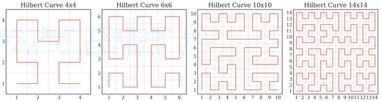
Figure 1.
Generalized Hilbert curve of arbitrary size.
3. Methods
3.1. The Two-Step Framework of Pooling
To clearly articulate our proposed LDS3Pool method and position it within the context of existing pooling research, we adopt the conceptual framework introduced by Zhai et al. [], which decomposes standard pooling operations (specifically those where stride s equals pooling window size ) into two discrete steps. This “two-step decomposition” framework helps to clearly separate the local feature aggregation from spatial downsampling components of pooling, highlighting how different pooling strategies primarily differ in their approach to spatial downsampling.
Throughout this paper, we use the following notation conventions: Calligraphic letters (e.g., , ) denote functions or point sets; bold uppercase letters (e.g., , ) represent feature maps or matrices; bold lowercase letters (e.g., , ) represent individual points, vectors, or array indices; and non-bold lowercase letters (e.g., s) represent scalar values. Subscripts indicate indices or coordinates (e.g., is the pixel at position ), while superscripts denote alternative versions or transformations (e.g., is the intermediate feature map).
Let the input feature map for each channel be , where H and W represent the feature map’s height and width, respectively. Following the perspective proposed by Zhai et al. [], standard pooling (with stride s) can be understood as a combination of two consecutive steps:
- Step1: Local Feature Aggregation
- Apply a local aggregation function with a receptive field of and stride 1 over the input feature map (with appropriate padding if necessary).
- This step generates an intermediate feature map with dimensions matching or nearly matching the input. Specifically:
- Each pixel represents an aggregated summary of information from the neighborhood centered at (or starting from) position in the original input . Common aggregation functions include maximum (Max), average (Average), or even learnable functions in some methods.
- Step 2: Spatial downsampling
- Apply a spatial downsampling function to the intermediate feature map .
- This step reduces the spatial dimensions from to , where and (assuming H and W are divisible by s). That isproducing the final pooling output .
- The critical distinction lies in how is implemented: This function determines which pixel values from are selected and how they are combined to constitute the final output . This is where different pooling strategies fundamentally diverge in their spatial processing approach.
This two-step decomposition helps clarify the essential differences between pooling methods. For standard MaxPool or AvgPool, the first step typically involves taking the maximum or average value within each window to generate the intermediate feature map . The second step—spatial downsampling—is deterministic: for example, selecting the value at the top-left corner of each region in to form the final output.
Stochastic pooling [] introduces randomness primarily in the first step by randomly sampling a value for aggregation based on activation magnitudes within the window while typically maintaining a deterministic spatial downsampling approach similar to MaxPool in the second step.
In contrast, S3Pool [] incorporates randomness into the second step—the spatial downsampling phase. It first completes the aggregation step using a deterministic Max method to obtain then performs random spatial sampling by dividing the feature map into grids and randomly selecting row and column indices to determine which pixels from will contribute to the final output .
Thus, while various methods can be framed within this decomposition, they differ fundamentally in where they introduce randomness (in the value aggregation phase or the spatial sampling phase) and in their spatial sampling strategy (deterministic or random and the specific implementation of randomness).
3.2. Quasi-Random Spatial Sampling with Low-Discrepancy Sequences
As noted previously, S3Pool [] introduces spatial randomness by dividing the feature map into grids and randomly selecting rows and columns within each grid. While effective for enhancing generalization, this approach strongly depends on the manually tuned grid size parameter g, which can significantly impact performance and requires careful adjustment for different network layers and feature map sizes. Moreover, S3Pool does not provide theoretical guarantees regarding the uniformity of its spatial sampling, potentially introducing coverage biases.
To address these limitations, we propose LDS3Pool, a novel pooling strategy that leverages low-discrepancy sequences (LDSs) for spatial downsampling. LDSs, also known as quasi-random sequences, are deterministically generated sequences designed to achieve more uniform coverage of sampling spaces than purely random or pseudo-random approaches [].
The key insight of our approach is that LDSs provide a mathematically principled middle ground between fully deterministic and purely stochastic sampling—their construction ensures minimal deviation between the empirical distribution of sampled points and the uniform distribution. This deviation, formally quantified as discrepancy, decreases at a rate of for an LDS compared to the rate of pseudo-random sequences, providing theoretically superior domain coverage with fewer samples [].
This property makes LDSs ideal for guiding spatial sampling in CNN pooling layers, introducing beneficial randomness while maintaining mathematical guarantees of sampling quality.
3.3. The LDS3Pool Algorithm
Figure 2 illustrates the proposed LDS3Pool in the structure of two-step decomposition and provides an intuitive comparison with the control group methods. The specific steps are given below:
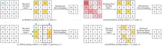
Figure 2.
The two-step decomposition of proposed LDS3Pool and three classical pooling methods. The yellow fill represents the pixels selected by the sampling step, while the red fill in diagram (b) indicates the probability of a pixel being chosen in the random sampling.
- Step 1: Local Feature Aggregation
Similar to standard pooling methods, we first apply a max pooling operation with stride 1 and window size to the input feature map to obtain an intermediate feature map : .
- Step 2: Hilbert Curve-based Pixel Ordering
Instead of directly sampling rows and columns, we map the 2D positions of pixels in the feature map to a 1D sequence using a generalized Hilbert space-filling curve []. This generalized approach allows us to handle feature maps of arbitrary sizes, not just those with dimensions that are powers of two. To perform this mapping,
- Denote each pixel in as ; then, all the pixels in constitute an disordered point set: .
- Generate a generalized Hilbert curve of the same size as . has vertices, which are denoted as , and .
- Since there is a one-to-one correspondence between the vertices on and the point coordinates in , the pixels in can be sorted according to the order of on , resulting in
This sorting transforms the 2D feature map into a 1D sequence that preserves spatial locality, with pixels close in 2D space remaining close in the 1D ordering.
To avoid redundant calculations, the vertex sequence of is generated when the pooling layer of the CNN is built and called directly during forward propagation. In this way, pixel sorting introduces only limited additional computation.
- Step 3: LDS-based Quasi-Random Sampling
To achieve quasi-random sampling with theoretical uniformity guarantees, we apply a low-discrepancy sequence to select indices from the Hilbert-ordered pixel sequence:
- Generate an LDS of length using the additive recurrence relation based on Euler’s number e:where represents the i-th value in the LDS.
- Create a sorted version of this sequence and compute the inverse sorting vector , so thatThis vector maps each original index i to its position in the sorted LDS.
- Reorder the Hilbert-ordered pixel sequence using the inverse sorting vector:
- Randomly pick a start index t and select coordinates from the reordered sequence:
Note that instead of pixels are sampled. This factor of 2 represents a fixed oversampling strategy inherent to our LDS3Pool implementation, providing a richer set of candidates for the reconstruction step. The effectiveness of this choice is validated empirically in our ablation studies (Section 4.1.3 and Section 4.3), where we compare it against sampling different numbers of points.
In the training phase, t is generated by a random number seed generator and varies in each forward propagation process. In the validation state (inference state), to obtain definite results and simplify calculations, we fix ; that is, we take the first M pixels of .
To avoid redundant calculations, the LDS will also be pre-generated when the size layer is built.
- Step 4: Feature Map Reconstruction
Finally, the downsampled feature map is reconstructed using the following procedure:
- Copy with the same dimensions as , initialized with zeros.
- For each selected coordinate , set: .
- Apply a standard max pooling operation with window size and stride s to this sparse feature map: . This produces the final downsampled feature map .
Algorithm 1 summarizes the process of LDS3Pool.
| Algorithm 1 LDS3Pool: Pooling with Quasi-Random Spatial Sampling |
| Require: Input feature map , pooling window size s, stride s |
| Ensure: Pooled feature map |
|
3.4. Illustration of LDS3Pool
Figure 3 illustrates the steps of ordering and quasi-random sampling, and Figure 4 presents the feature map reconstruction step on a naive feature map. For visual simplicity and easier comparison of the underlying mechanisms, these figures depict the selection and reconstruction based on points. However, as discussed and validated in our ablation study (Section 4.3), our final LDS3Pool implementation utilizes an oversampling factor of 2 (i.e., selecting points) to achieve optimal performance. The core principles of Hilbert ordering, LDS-guided selection, and feature map reconstruction remain the same.
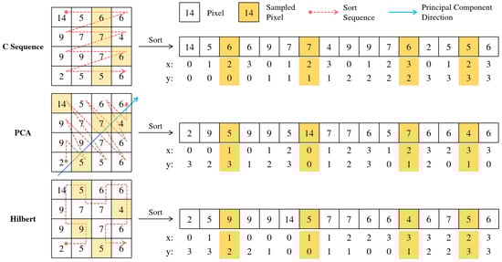
Figure 3.
The different ordering schemes (C-order, PCA-based, and Hilbert curve) and the resulting sampling patterns. (For illustrative clarity, this example shows the selection of points based on the ordering. The actual LDS3Pool implementation uses , as explained in Section 3.3 and validated in Section 4.3).
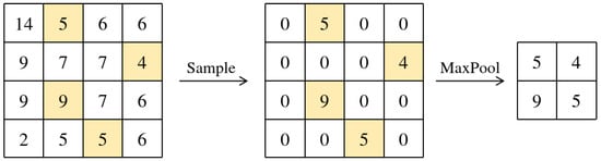
Figure 4.
Feature map reconstruction process.
Take and generate the LDS inverse sorting vector:
Then .
Figure 3 compares LDS3Pool-Hilbert to two ordering alternatives as well:
- Simple C-ordering (row-major traversal) is used to linearize the 2D feature map.
- Principal component analysis is used to project pixel coordinates onto the first principal component direction for ordering.
The contribution of the Hilbert curve was verified in the ablation experiment.
Figure 5 visually compares the effects of applying different pooling methods directly to an example image. MaxPool retains sharpness but can create blockiness, while AvgPool smooths details, resulting in blurriness. The stochastic methods, S3Pool and LDS3Pool, introduce distinct visual artifacts reflecting their underlying random grid-based and quasi-random point-based sampling strategies, respectively. Note that visual fidelity here may not directly correlate with performance on learned feature maps.
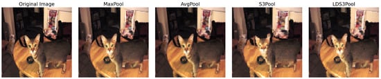
Figure 5.
Visual effect of LDS3Pool and three classical pooling methods.
3.5. Theoretical Analysis
The superior performance of the LDS3Pool method derives from the synergistic combination of two mathematically principled components: the locality-preserving properties of Hilbert curve ordering and the uniform coverage guarantees of low-discrepancy sequences. This section provides a quantitative analysis of both aspects.
3.5.1. Locality Preservation Analysis of Ordering Schemes
The initial step of the LDS3Pool algorithm, linearizing the 2D feature map, is critical for preserving the spatial structure inherent in the data. The choice of an ordering scheme directly impacts how local neighborhoods are maintained. To formally justify the selection of the Hilbert curve over simpler alternatives (e.g., C-ordering and PCA-based ordering), its locality preservation property is quantitatively analyzed.
A formal metric for this analysis is the Discrete Locality Measure, , adapted from prior work []. It quantifies the maximum distortion when mapping 2D coordinates to a 1D sequence:
where represents the 2D coordinate corresponding to the 1D index i, and is the Euclidean distance. A lower value signifies a better preservation of local structures.
For a raster scan (C-ordering) on an feature map, the locality measure is highly sensitive to the map’s dimensions. The worst-case distortion occurs at row transitions. Consider two spatially adjacent pixels: and . Their 1D index distance is minimal, . However, their squared Euclidean distance is . This results in an value on the order of .
A PCA-based ordering exhibits a comparably poor locality measure. For a grid of pixel coordinates, the eigenvectors of the covariance matrix are and . Consequently, when , PCA ordering degenerates to a raster or column scan. In the common case where , any direction can be chosen as the principal component. If the diagonal direction is chosen, considering the points and , their squared Euclidean distance is , and the ratio becomes . This quadratic degradation means that for larger feature maps, these simple ordering schemes fail to preserve local neighborhoods effectively.
In stark contrast, the 2D Hilbert curve possesses a remarkable theoretical property. As established in the literature, its value is bounded by a small, size- independent constant:
This property is demonstrated by Gotsman and Lindenbaum [] and is a key advantage over other space-filling curves like the Peano curve, which has a higher bound of 8.
This exceptional and robust locality preservation is the primary reason for selecting the Hilbert curve for LDS3Pool. In deep networks where feature map dimensions vary widely across layers, only an ordering scheme with a size-independent locality measure can guarantee that spatial relationships are consistently maintained, providing a stable and meaningful input for the subsequent quasi-random sampling step.
3.5.2. Uniform Coverage Guarantees of Low-Discrepancy Sequences
Low-discrepancy sequences (LDSs) are specifically designed to achieve superior uniform coverage of a sampling domain compared to pseudo-random sequences. Their fundamental property is the minimization of discrepancy, which formally quantifies the deviation between the empirical distribution of a finite point set and the uniform distribution. For a point set of N points in a space with Lebesgue measure , the star discrepancy is defined as
where the supremum is taken over all anchor boxes J in the m-dimensional unit hypercube. While pseudo-random sequences exhibit a discrepancy that decreases at a rate of , LDSs are constructed to achieve a much faster convergence rate, typically . This mathematical guarantee of uniformity is the core reason for their use in quasi-random sampling.
A key insight for the LDS3Pool algorithm is how this property can be transferred to a discrete, ordered set, such as the Hilbert-ordered feature map pixels. An LDS generates a sequence of points that are evenly distributed. The inverse sorting vector derived from this sequence effectively acts as a permutation that reorders the original indices in a way that mimics this uniformity.
Consequently, when a contiguous block of indices is selected from this reordered sequence (as is performed during the training phase of LDS3Pool by choosing a random starting point t), the corresponding subset of pixels is guaranteed to be well-distributed across the entire Hilbert curve path. This ensures that any sampled subset, regardless of the random starting point, provides a comprehensive and representative view of the entire feature map, avoiding the clustering and gaps that can occur with purely random sampling. The specific LDS employed in this work, based on the additive recurrence , is a type of Kronecker sequence known for its strong theoretical properties and computational efficiency [].
3.5.3. Synergistic Combination and Empirical Validation of Uniformity
The effectiveness of LDS3Pool stems from the synergistic combination of the two principles analyzed above. The Hilbert curve ordering transforms the unstructured 2D feature map into a spatially coherent 1D sequence, creating a “spatial path” that preserves neighborhood relationships. Subsequently, applying LDS-based sampling along this path ensures that the selected points are evenly distributed across the entire spatial domain, avoiding the clustering and gaps inherent in pseudo-random selection.
To empirically validate the superior spatial uniformity provided by this synergistic approach, a comparative experiment was conducted. A grid, representing a typical feature map, was downsampled at a rate of (selecting 1024 out of 4096 points) using three different strategies: LDS3Pool, Simple Random Sampling (SRS), and S3Pool with varying grid sizes ().
The resulting spatial distributions of the sampled points are visualized in Figure 6. As observed, the points generated by LDS3Pool exhibit the highest degree of visual uniformity. To quantify this, the standard deviation of the local sampling density across all possible sliding windows was calculated. A lower standard deviation indicates a more homogeneous distribution.
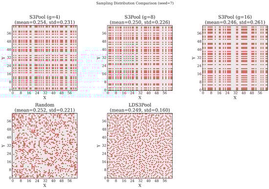
Figure 6.
Visualization of spatial distributions for different sampling strategies (seed = 7). LDS3Pool demonstrates superior uniformity, avoiding the clusters and voids present in SRS and the grid-artifacts of S3Pool.
The quantitative results, summarized in Table 1, confirm the visual findings. While all methods achieve the expected mean density of approximately 0.25, LDS3Pool yields a significantly lower average standard deviation (0.165) compared to both SRS (0.218) and all variants of S3Pool. This provides strong empirical evidence that the combination of Hilbert curve ordering and LDS-based selection produces a more uniform and representative spatial sample. This enhanced uniformity ensures that the downsampled feature map provides a comprehensive and unbiased view to subsequent network layers.

Table 1.
Statistics of local sampling density (mean and standard deviation) for different sampling strategies, averaged over three random seeds. The lowest standard deviation, indicating the best uniformity, is highlighted in bold.
3.5.4. Computational Complexity Analysis
The computational complexity of LDS3Pool can be analyzed in terms of both its initialization phase (one-time cost) and its forward pass during training and inference (recurring cost). This analysis helps elucidate the practical trade-offs between improved model accuracy and additional computational burden.
- Initialization Phase Complexity
During initialization, LDS3Pool performs two main pre-computation steps ( represents the total number of elements in a feature map of size ):
- Hilbert Curve Generation: The recursive Hilbert curve generation for an input feature map has a time complexity of . The logarithmic factor arises from the recursion depth of approximately needed to traverse all N points through recursive subdivision. This operation is computed only once during model initialization and stored for future use, thus not impacting training or inference time.
- Low-Discrepancy Sequence Generation: Computing the LDS based on the additive recurrence relation has a time complexity of for sequence generation followed by for sorting operations. This is also a one-time cost during initialization.
The space complexity for storing both the Hilbert curve mapping and the LDS inverse sorting vector is , proportional to the size of the feature map.
- Forward Pass Complexity During the forward pass of LDS3Pool, the computational operations can be broken down as follows:
- Local Feature Aggregation: The max pooling operation with stride 1 and window size on an input feature map has a time complexity of , which is asymptotically equivalent to standard max pooling.
- Sampling and Feature Map Reconstruction:
- The random selection of a start index for the LDS sampling is .
- Creating a sparse feature map using the selected coordinates is , where k is the oversampling factor (2 in our implementation).
- The final max pooling operation with stride s is .
The key insight is that most of the computational overhead compared to standard pooling comes from the need to create and apply a boolean mask to the feature map. However, these operations can be efficiently implemented using scatter operations in modern deep learning frameworks.
Since the pooling window size s is typically a small constant (usually 2), and the oversampling factor k is also a fixed constant, the overall time complexity of the forward pass is , which is the same asymptotic complexity as standard pooling operations. The difference lies in the constant factors and the actual number of operations performed.
The practical overhead measurements are provided in Section 4.6, where we compare the training and inference times across different pooling methods.
4. Experiments
4.1. Experiment Setup
To comprehensively validate the proposed LDS3Pool method, a multi-stage experimental evaluation was designed. The initial experiments focus on a detailed performance comparison against baseline methods on classic CNN architectures. This is followed by a series of ablation studies to dissect the contributions of LDS3Pool’s key components. Finally, to assess its practical applicability and generalization capability, the best-performing variant of our method is benchmarked on a modern ResNet architecture. This systematic approach allows for a thorough analysis of both the method’s effectiveness and its underlying mechanisms.
4.1.1. Datasets
We selected six diverse image classification benchmarks that span a wide range of image sizes, channel counts, and classification complexities. This diversity allows us to evaluate how LDS3Pool performs across different feature scales and dataset characteristics:
- MNIST and FashionMNIST: Single-channel grayscale images of size pixels, each containing 10 classes with 60,000 training and 10,000 validation images. MNIST contains handwritten digits, while FashionMNIST features clothing items [,].
- CIFAR10 and CIFAR100: Three-channel RGB images of size pixels, containing 50,000 training and 10,000 validation images. CIFAR10 includes 10 common object classes, while CIFAR100 extends this to 100 more fine-grained categories [].
- STL10: Higher-resolution RGB images of size pixels, comprising 10 classes with 5000 training and 8000 validation images, focused on animals and transportation vehicles [].
- OxfordIIITPet: Large RGB images uniformly resized to pixels, containing 37 pet breeds consolidated into a binary cat/dog classification task. The dataset includes 3680 training and 3669 validation images [].
This selection provides a comprehensive testbed ranging from small grayscale digits to detailed high-resolution pet photographs, enabling evaluation of LDS3Pool’s performance across varying image complexities and spatial scales.
Table 2 summarizes the key characteristics of these datasets, and Figure 7 displays representative sample images from each dataset.
Table 2.
Key characteristics of the datasets used in our experiments.
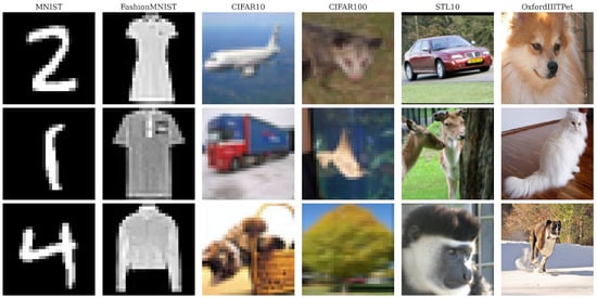
Figure 7.
Sample images from each of the six datasets used in the experiments.
4.1.2. Network Architectures
To evaluate LDS3Pool across different network depths and architectural patterns, we implemented two classical convolutional neural network architectures:
- LeNet5: A relatively shallow architecture originally designed for digit recognition, consisting of two convolutional layers followed by three fully connected layers, with two pooling operations []. This network serves as our lightweight model for experiments with smaller datasets.
- VGG11: A deeper architecture featuring eight convolutional layers organized in blocks, with five pooling operations and three fully connected layers []. This network provides a more complex testbed for evaluating pooling performance in deeper architectures.
These two networks are chosen for their simple and transparent designs. These architectures allow us to isolate and clearly analyze the specific contributions of different pooling strategies without confounding factors from complex residual connections, attention mechanisms, or normalization techniques.
In both networks, each pooling layer is replaced with the pooling methods under study (i.e., the proposed LDS3Pool and control groups in Section 4.1.3) while maintaining all other architectural elements. Each pooling operation uses a window size of with stride 2, which represents the most common pooling configuration in modern CNN architectures.
Figure 8 illustrates the architectural details of both networks with the specific layer configurations.
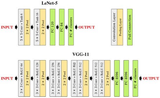
Figure 8.
Network architecture diagrams for LeNet5 and VGG11, highlighting the pooling layers that are replaced in our experiments.
To facilitate comprehensive evaluation across different feature map scales, we matched networks to datasets as follows:
- LeNet5 was applied to MNIST, FashionMNIST, CIFAR10, and CIFAR100.
- VGG11 was applied to CIFAR10, CIFAR100, STL10, and OxfordIIITPet.
This pairing ensured that LDS3Pool was tested on feature maps of various sizes, from as small as to as large as , providing insights into its performance across the full spectrum of practical application scenarios.
Table 3 details the feature map sizes at each pooling layer for our experimental configurations, demonstrating the diversity of spatial scales tested.
Table 3.
Feature map sizes at each pooling layer across different network–dataset configurations.
In addition to these classic models, a modern architecture, ResNet18 [], was employed as detailed in Section 4.4 to specifically evaluate the generalization performance of LDS3Pool in a contemporary deep learning pipeline.
4.1.3. Control Experiments and Ablation Study
To rigorously evaluate LDS3Pool’s performance and isolate the contributions of its key components, we designed a comprehensive set of control experiments and ablation studies.
- Baseline Methods
- MaxPool: Standard max pooling, representing the most common deterministic approach.
- AvgPool: Standard average pooling, providing an alternative deterministic baseline.
- S3Pool: The stochastic spatial sampling pooling method that serves as our primary comparison point.
For S3Pool, we carefully configured the grid size parameter g based on recommendations from the original paper and preliminary optimization experiments to ensure fair comparison. In LeNet5, we set - to 2-2 for both pooling layers. For VGG11, we used the following configurations:
- CIFAR10/100: ---- = 16-8-4-2-2.
- STL10: ---- = 32-16-8-4-2.
- OxfordIIITPet: ---- = 56-28-14-7-7.
To obtain definite results, the validation phase of S3Pool was replaced with MaxPool (the original paper used AvgPool, but in pre-experiments, MaxPool was observed to achieve higher validation set accuracy).
The implementation of S3Pool is adapted from Zhai’s [] code (from Theano to PyTorch (Version 2.5.1) []).
- Ablation Study on Ordering
To isolate the specific contribution of the Hilbert curve ordering in our method, we implemented three variants of LDS3Pool that differ only in the pixel ordering strategy (Step 2 in our algorithm):
- LDS3Pool-C uses simple C-ordering (row-major traversal) to linearize the 2D feature map.
- LDS3Pool-PCA uses principal component analysis to project pixel coordinates onto the first principal component direction for ordering.
- LDS3Pool-Hilbert, our proposed method, uses Hilbert curve ordering for linearization.
- Ablation Study on Oversampling
To verify the significance of selecting redundant data points in Step 3 of Section 3.3, the following ablation experiment was designed: Let (where k denotes the oversampling ratio), and sequentially take k as .
Training was performed on four networks/datasets combinations, LeNet5/MNIST, LeNet5/CIFAR10, VGG11/STL10, and VGG11/OxfordIIITPet (including shallow and deep networks, grayscale and color images, and various size of images), and their highest validation set accuracy was compared. Considering the common pooling size , means selecting the minimum pixels required for reconstruction, and means selecting all the data points.
4.1.4. Training Setup
We established a consistent training protocol across all experiments to ensure fair comparison:
- Loss Function: Cross-entropy loss.
- Optimizer: Adam with initial learning rate of 0.001 [].
- Learning Rate Schedule: StepLR scheduler with step size 10 and decay factor () of 0.5.
- Batch Size: 32 for all experiments.
- Training Duration: 150 epochs for OxfordIIITPet, 100 epochs for all other datasets.
- Evaluation Metric: Maximum validation accuracy achieved during training and generalization gap between the training accuracy and the validation accuracy.
To mitigate the effects of random initialization and stochastic training elements, we conducted each experiment with six different random seeds (7, 42, 123, 1309, 5287, and 31,415) and reported the average performance across these runs. This procedure ensures the robustness of our findings against random variations.
All experiments were conducted on a workstation equipped with an NVIDIA RTX A4000 GPU using the PyTorch framework. Note that our objective is not to achieve state-of-the-art performance on these datasets but rather to perform controlled comparisons between different pooling strategies under identical conditions. This approach isolates the specific impact of the pooling method on model performance.
4.2. Main Results on Classic Architectures
Table 4 presents the maximum validation accuracy (averaged across six random seeds) for each combination of network, dataset, and pooling method. Table 5 shows the corresponding coefficient of variation (CV). The visual expression is given in Figure 9.
Table 4.
Validation accuracy achieved by different pooling methods (highest accuracy is highlighted in bold).
Table 5.
Validation accuracy coefficient of variation (lowest value is highlighted in bold).
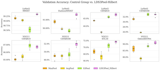
Figure 9.
Validation accuracy box chart for each network/dataset. The black dots represent the outlier data points.
Based on the numerical results, the following information can be obtained:
- Across all models and datasets, LDS3Pool-Hilbert consistently achieved the highest or near-highest validation accuracy, outperforming S3Pool, MaxPool, and AvgPool in overall ranking. This confirms the effectiveness of introducing principled randomness for performance enhancement.
- LDS3Pool-Hilbert demonstrated significant accuracy improvements over all baselines. Notably, it improved upon the classic MaxPool by up to 5 percentage points (on VGG11/OxfordIIITPet) and upon the stochastic S3Pool by 1–3 percentage points in many cases. Given that only the pooling layer was modified, these gains are considerable.
- The average coefficient of variation (CV) for LDS3Pool-Hilbert and S3Pool falls between that of MaxPool and AvgPool. This indicates that introducing randomness via these methods does not negatively impact the stability of the training results.
- LDS3Pool-Hilbert generally exhibits a slightly lower average CV than S3Pool, with significantly lower variability on several key configurations (e.g., VGG11/STL10). This suggests that its quasi-random approach offers more controllable randomness, leading to a more stable and representative downsampling of the feature map.
The statistical significance of these improvements was assessed through paired t-tests comparing LDS3Pool-Hilbert against each baseline method: Table 6 shows the paired T-tests of the six repeated experiments of the two pooling methods on each network and dataset. Table 7 shows the paired T-tests of the two pooling methods on eight combinations of network and dataset. The tables verifies the superiority of LDS3Pool-Hilbert.
Table 6.
Statistical significance of accuracy improvements: on six repeat runs of each network–dataset combination (* denotes and ** denotes ).
Table 7.
Statistical significance of accuracy improvements: across eight network–dataset combinations (* denotes and ** denotes ).
- Per-Configuration Analysis: LDS3Pool-Hilbert demonstrates a statistically significant advantage over the baseline methods in most cases, often with . It is noted that in two specific cases (LeNet5/CIFAR100 and VGG11/CIFAR10), the performance difference compared to S3Pool was not significant, which indicates that the two methods are statistically indistinguishable in these specific settings. This suggests that for certain less complex dataset–architecture combinations, the simpler randomization of S3Pool may already provide a sufficient regularization effect.
- Overall Analysis: When aggregating the results across all eight network–dataset combinations, paired t-tests confirm the overall superiority of LDS3Pool-Hilbert. It achieves a highly significant improvement over traditional MaxPool () and a significant improvement over both AvgPool and S3Pool ().
In summary, the proposed LDS3Pool-Hilbert method has significant advantages on networks of different sizes and output images of different sizes. Moreover, although it introduces randomness, it can still achieve stable convergence results.
4.3. Ablation Studies
4.3.1. Ablation Study on Ordering
To analyze the contribution of Hilbert ordering, Table 8 gives the average validation set accuracy of LDS3Pool variants based on different ordering methods on each network and dataset. Table 9 and Table 10 show paired t-tests for six repeated experiments and across eight network/dataset combinations, respectively. Table 11 presents the coefficient of variation. Figure 10 is a visualization.
Table 8.
Validation accuracy achieved by LDS3Pool with different ordering methods (the highest value is marked in bold).
Table 9.
Statistical significance of accuracy improvements brought by Hilbert ordering: on six repeated runs (* denotes and ** denotes ).
Table 10.
Statistical significance of accuracy improvements brought by Hilbert ordering: across eight network–dataset combinations (* denotes and ** denotes ).
Table 11.
Validation accuracy coefficient of variation on different ordering methods (the lowest value is marked in bold).
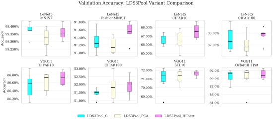
Figure 10.
Validation accuracy achieved by LDS3Pool with different ordering methods. The black dots represent the outlier data points.
The key findings include
- Superior Performance on Small Networks: On the small model LeNet5 (and the corresponding small-sized image datasets), Hilbert consistently achieved the highest average validation set accuracy (except on LeNet5/MNIST, where the three variants barely differ). This is particularly evident for CIFAR10, where Hilbert achieved 67.545% accuracy compared to 66.519% for PCA and 66.575% for C-ordering variants, representing a difference of approximately 1 percentage point. Similarly, on CIFAR100, Hilbert showed notable improvements. The paired t-test results confirm that the accuracy improvements of Hilbert relative to C-order are statistically significant on FashionMNIST (p < 0.01) and CIFAR10 (p < 0.01), while improvements over PCA are significant on FashionMNIST (p < 0.05) and CIFAR100 (p < 0.05).
- Consistent Advantages on Larger Networks: On the larger VGG11 model, the Hilbert variant still outperforms the other two across all datasets. Especially on OxfordIIITPet with the largest image size, Hilbert achieves accuracy of 91.012%, outperforming PCA (90.131%) by about 1 percentage point. While the paired t-test results indicate that these differences on the VGG11 model are not statistically significant, they highlight that the Hilbert ordering provides the most substantial benefits when working with smaller feature maps where spatial structure preservation is particularly critical.
- Overall Advantages: Paired tests on the results of eight network–dataset combinations also verify that Hilbert ordering has extraordinary improvement over C-sequence (); it also has a significant improvement over PCA ordering ().
- Enhanced Stability Across Configurations: On multiple network–dataset pairs (LeNet5/CIFAR10, VGG11/CIFAR10, VGG11/STL10, and VGG/OxfordIIITPet), the Hilbert variant achieved the lowest CV. In addition, the Hilbert variant achieved the lowest average coefficient of variation, while the average coefficient of variation of the PCA variant and the C-Sequence variant were almost the same.
In summary, this experiment verifies the contribution of the Hilbert curve to LDS3Pool: The Hilbert variant delivers statistically significant improvements in validation accuracy on smaller networks and demonstrates consistent advantages on larger models as well, with gains of up to 1 percentage points on datasets like OxfordIIITPet. Additionally, the Hilbert ordering provides more stable results across repeated experiments, as evidenced by its lower coefficient of variation. These findings confirm that Hilbert curve-based linearization effectively preserves local spatial relationships in feature maps across various network scales and dataset complexities.
4.3.2. Ablation Study on Oversampling
The following analyzes the contribution of oversampling to the model. Table 12 gives the average validation set accuracy on the four representative network/dataset pairs when oversampling is performed at different ratios k, while Figure 11 shows the change in accuracy versus k. Note that this ablation experiment was performed separately, so the values at may differ slightly from the main experiment results in Figure 3.
Table 12.
Validation accuracy for different k-values on various network–dataset configurations (the top value is highlighted in bold).
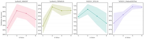
Figure 11.
Validation accuracy versus oversampling ratio k (the semi-transparent area indicates the standard deviation).
The main findings include
- Benefit of moderate oversampling: Across all four tested configurations, increasing the sampling factor from (minimal sampling) to resulted in a significant improvement in validation accuracy. This demonstrates that providing the reconstruction step with more candidate pixels is clearly beneficial, likely allowing the final MaxPool operation to select more representative high activations from each region.
- Parabolic trend: The optimal performance was achieved at for three out of the four pairs: LeNet5/MNIST, LeNet5/CIFAR10, and VGG11/STL10, while for VGG11/OxfordIIITPet, the peak accuracy occurred at . Performance generally decreases or plateaus after reaching the optimal k. This indicates diminishing returns from further increasing the sampling density. At (representing full sampling when ), the process potentially loses the regularization benefits gained from the quasi-random selection process at lower k values.
- Core method effectiveness: Even with minimal sampling (), the validation accuracy achieved by LDS3Pool is higher than or close to the best results obtained by the baseline methods reported in Table 3 for the corresponding network/dataset pairs. This underscores the inherent effectiveness of the Hilbert-ordered and LDS-guided spatial sampling strategy, independent of the oversampling factor.
These findings confirm that moderate oversampling significantly enhances LDS3Pool’s performance. While the precise optimum varied slightly ( or ) depending on the specific configuration, consistently provided a major improvement over and was optimal in the majority (3 out of 4) of the diverse scenarios tested. It represents the simplest factor that yields substantial gains. Therefore, to maintain consistency and utilize a generally robust and effective setting across the different network architectures and dataset scales presented in our main experimental results (Section 4.2), we adopted as the standard oversampling ratio in our LDS3Pool implementation.
4.4. Generalization Study on Modern Architectures
Having established the general effectiveness of LDS3Pool on classic architectures and identified its optimal configuration through ablation studies, this section aims to evaluate its generalization capability in a modern deep learning context. To this end, experiments were conducted on the ResNet18 architecture [], a standard backbone in computer vision. Based on the findings in Section 4.3, the best-performing variant, LDS3Pool-Hilbert with an oversampling factor of , was used for this evaluation.
A key feature of ResNet is its use of strided convolutions for downsampling. To create a controlled comparison aligned with the two-step pooling framework presented in this paper, a key mathematical property is leveraged: a convolution (stride = 2) layer is equivalent to a convolution (stride = 1) layer followed by a simple top-left pixel selection. This implicit downsampling step, a form of systematic sampling, is termed the Ordered System Sampling Pool (OSSPool). Such a decomposition allows the downsampling strategy to be isolated as the sole variable. In the experiments, this OSSPool was replaced with other explicit pooling methods (MaxPool, AvgPool, S3Pool, and LDS3Pool) for a direct comparison of their effectiveness.
The experimental results on four challenging datasets are presented in Table 13. Each experiment was repeated six times with different random seeds to ensure robust conclusions.
Table 13.
Validation accuracy (%) on ResNet18. The best performance is highlighted in bold.
The results, presented in Table 13, clearly demonstrate that LDS3Pool-Hilbert continues to deliver superior performance on the ResNet18 architecture. Across all four datasets, our method achieved the highest average validation accuracy. The statistical significance of these improvements is confirmed in Table 14, which shows that LDS3Pool-Hilbert holds a statistically significant advantage ( or ) over the baselines in most cases.
Table 14.
Statistical significance (t-values) of accuracy improvements for LDS3Pool-Hilbert against baseline methods on ResNet18. Comparisons are from paired t-tests on six repeat runs (* denotes and ** denotes ).
Several key insights can be drawn from these results:
- Potential for Enhancement over the ResNet Baseline. LDS3Pool-Hilbert shows a statistically significant performance gain over the OSSPool baseline across all datasets. The OSSPool baseline, which mirrors the highly efficient, integrated downsampling of the original ResNet, serves as a strong reference. The performance uplift achieved by replacing it suggests that when the downsampling step is explicitly decoupled from the convolution, there is an opportunity to enhance performance by employing more sophisticated sampling strategies. This is further supported by the observation that even standard MaxPool and AvgPool, which aggregate information from a full local window, outperform the simple pixel selection of OSSPool.
- Robustness and Consistency. While some baseline methods show strong performance on specific datasets (e.g., S3Pool on CIFAR10, MaxPool on OxfordIIITPet), none demonstrate universal effectiveness. In contrast, LDS3Pool-Hilbert emerges as the most consistent top-performing strategy across all four diverse datasets. This highlights its robustness and adaptability as a general-purpose downsampling module.
- A More Balanced Approach to Regularization. The comparison with S3Pool reveals a key advantage in how randomness is applied. S3Pool’s performance, while strong in some cases, shows notable instability, with a significant performance drop on CIFAR100 and OxfordIIITPet. LDS3Pool-Hilbert, however, maintains consistent and significant gains. This indicates that its structured, quasi-random approach strikes a more effective balance, achieving the benefits of stochastic regularization without sacrificing the performance stability that is crucial for reliable model training.
These findings strongly support the practical applicability of LDS3Pool as a drop-in improvement for contemporary deep learning pipelines.
4.5. Analysis of Overfitting Mitigation
An important claim of this work is that the principled randomness of LDS3Pool acts as an effective regularizer. This section analyzes this property by examining the learning dynamics and quantifying the generalization gap.
Figure 12 illustrates the training and validation accuracy trends for three representative experimental setups, spanning classic shallow, classic deep, and modern deep architectures. The light-colored thin lines represent the raw data, while the dark-colored thick lines show the smoothed trends.
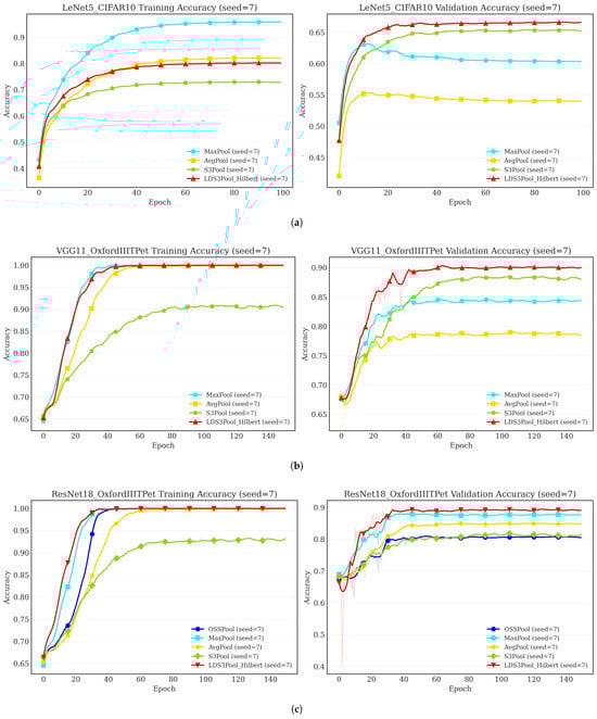
Figure 12.
Accuracy trends of the training set (left) and validation set (right) for different architectures and datasets. (a) A shallow network prone to overfitting. (b) A deep classic network on a complex task. (c) A modern network on a complex task.
The learning curves reveal a consistent pattern. In the LeNet5/CIFAR10 experiment (Figure 12a), where overfitting is most pronounced, the validation accuracy of the deterministic MaxPool and AvgPool methods stagnates early, while their training accuracy continues to climb. In contrast, both S3Pool and LDS3Pool-Hilbert effectively mitigate this, showing sustained improvement or stability in validation accuracy.
In the more complex VGG11 and ResNet18 experiments on the OxfordIIITPet dataset (Figure 12b,c), while severe overfitting is less apparent, the learning efficiency differs. LDS3Pool-Hilbert consistently demonstrates a strong and sustained learning trajectory, ultimately achieving the highest validation accuracy.
To provide a quantitative measure of this regularization effect, the generalization gap was calculated for all experimental setups, defined as the difference between the final training and validation accuracy. A smaller gap signifies better generalization.
Table 15 provides strong quantitative support for the visual analysis. The deterministic methods, MaxPool and AvgPool, consistently exhibit a large generalization gap, confirming their tendency to overfit. The stochastic methods, in contrast, show a clear advantage in mitigating this issue.
Table 15.
Generalization gap (training accuracy-validation accuracy) for various models and datasets. A smaller value indicates better regularization. The results are averaged on 6 runs.
The comparison between S3Pool and LDS3Pool-Hilbert is particularly insightful. In nearly all scenarios, S3Pool yields the smallest numerical gap. However, this is frequently accompanied by lower overall validation accuracy (as seen in Table 4 and Table 13), suggesting its strong regularization can sometimes lead to underfitting by overly constraining the model’s learning capacity.
LDS3Pool-Hilbert, however, strikes a more effective balance. It consistently and substantially reduces the generalization gap compared to the deterministic baselines, achieving a sweet spot between regularization and feature preservation. While its gap may be numerically larger than S3Pool’s in some cases, it accomplishes this regularization without compromising the model’s ability to learn effectively. This allows LDS3Pool-Hilbert to converge to a significantly higher final validation accuracy. This synergy of high accuracy and robust generalization underscores the effectiveness of its principled quasi-random sampling strategy.
4.6. Computational Efficiency
In order to evaluate the application feasibility of LDS3Pool, its training time and inference time were compared with the three control group methods. In the training phase, a warm-up of one epoch was performed first, and then six epochs were trained. The average time of the epoch was calculated to provide a reasonable reference for the training cost. During inference, six inference phases were employed for the validation set, and the average batch time was calculated to measure the inference latency in the application scenario. The results are shown in Table 16 and Table 17.
Table 16.
Time consumption per epoch in training (s).
Table 17.
Time consumption per batch in inference (ms).
The following information can be obtained from the data:
- Training Overhead: During the training phase, the stochastic methods, S3Pool and LDS3Pool, introduce additional computational time compared to the deterministic baselines. This is expected, as they require extra operations for random index generation and sparse feature map construction. Across all architectures, including ResNet18, S3Pool consistently brings the largest overhead (approximately 50–60% compared to MaxPool), while LDS3Pool’s overhead is more moderate (approximately 20–35%).
- Inference Overhead: During the inference phase, S3Pool reverts to using MaxPool, thus showing no additional latency. LDS3Pool, however, maintains its sampling mechanism, resulting in a noticeable overhead. This overhead is more pronounced for deeper networks with larger feature maps, such as VGG11 and ResNet18.
In summary, while LDS3Pool introduces a moderate computational overhead, its application remains feasible. The additional latency during inference is generally small in absolute terms and may not be a bottleneck for many applications. Given the significant and consistent improvements in accuracy and generalization across all tested architectures, this trade-off is highly favorable. Furthermore, as this study focuses on the conceptual gains of the proposed sampling strategy, the implementation has not been deeply optimized. There is considerable potential for future work to accelerate these operations, for instance, through customized GPU kernels, which could further enhance the practical value of LDS3Pool.
5. Conclusions and Limitations
5.1. Conclusions
This paper introduced LDS3Pool, a novel pooling method that bridges the gap between deterministic and purely stochastic approaches by leveraging low-discrepancy sequences for quasi-random spatial sampling. The key innovation of LDS3Pool lies in its synergistic combination of Hilbert curve ordering for locality preservation and LDS-based selection for uniform coverage. This principled approach introduces beneficial regularization while maintaining crucial feature map structures.
The theoretical analysis provided a solid mathematical foundation for this design. By employing the Discrete Locality Measure, it was quantitatively demonstrated that Hilbert curve ordering offers a size-independent, constant-bounded locality preservation, far superior to the quadratically degrading performance of simpler ordering schemes. Furthermore, the properties of low-discrepancy sequences were shown to guarantee a more uniform spatial sampling coverage compared to pseudo-random methods.
Extensive experimental validation was conducted across multiple datasets and a range of CNN architectures, from classic LeNet5 and VGG11 to the modern ResNet18. The results consistently demonstrated that LDS3Pool outperforms traditional deterministic methods (MaxPool, AvgPool), the purely stochastic S3Pool, and the native downsampling strategy of ResNet. The performance gains were statistically significant and particularly notable on more challenging datasets, highlighting LDS3Pool’s superior generalization capabilities. A key practical advantage is the elimination of sensitive hyperparameters like the grid size in S3Pool, making LDS3Pool inherently more robust and adaptive across different network layers and architectures.
In summary, LDS3Pool is a theoretically sound and empirically effective pooling method. By integrating principles from number theory and fractal geometry into a core component of CNNs, it enhances model generalization in a robust, adaptive, and computationally feasible manner.
5.2. Limitations and Future Works
Despite its demonstrated advantages, LDS3Pool has several limitations that present clear opportunities for future research:
- Performance Optimization: The current implementation introduces a moderate computational overhead. Future work could explore optimized GPU kernels to accelerate the sampling operations for efficiency-critical applications.
- Broader Applications: The method’s effectiveness in other vision tasks, such as object detection and semantic segmentation where fine-grained spatial information is crucial, remains a promising area for exploration.
- Robustness Evaluation: A comprehensive evaluation of LDS3Pool’s robustness under challenging conditions, such as domain shifts or adversarial attacks, is an important direction for future investigation.
- Adaptive Sampling: The oversampling factor is currently fixed. An adaptive approach that adjusts this factor based on feature complexity or network depth could further enhance performance.
- Synergistic Effects: A systematic investigation of combining LDS3Pool with other regularization techniques, like Dropout, could reveal beneficial synergistic effects.
By addressing these limitations, the utility of LDS3Pool can be further expanded. The underlying principles of quasi-random sampling could also inspire new designs beyond pooling, potentially influencing attention mechanisms, token selection in Vision Transformers, or network architecture search.
Author Contributions
Conceptualization, Y.M. and L.G.; methodology, Y.M.; validation, M.L.; formal analysis, Y.M.; investigation, M.L.; resources, L.G.; data curation, Y.M.; writing—original draft preparation, Y.M.; writing—review and editing, L.G.; supervision, L.G.; project administration, L.G.; funding acquisition, L.G. All authors have read and agreed to the published version of the manuscript.
Funding
This work is supported by the Qilu Young Scholars Program Fund of Shandong University.
Data Availability Statement
The key scripts and data used in the experiments of this paper can be accessed at https://github.com/Yuening-Ma/LDS3Pool, accessed on 30 April 2025.
Acknowledgments
During the preparation of this manuscript, the authors used Claude 3.7 and Gemini 2.5 in the Introduction and Literature Review sections. Claude 3.7 was used for text editing as well. The authors have thoroughly reviewed and edited the output and take full responsibility for the content of this publication.
Conflicts of Interest
The funders had no role in the design of the study; in the collection, analyses, or interpretation of data; in the writing of the manuscript; or in the decision to publish the results.
References
- Saeedan, F.; Weber, N.; Goesele, M.; Roth, S. Detail-Preserving Pooling in Deep Networks. In Proceedings of the IEEE Conference on Computer Vision and Pattern Recognition (CVPR), Salt Lake City, UT, USA, 18–23 June 2018. [Google Scholar]
- He, K.; Zhang, X.; Ren, S.; Sun, J. Spatial pyramid pooling in deep convolutional networks for visual recognition. IEEE Trans. Pattern Anal. Mach. Intell. 2015, 37, 1904–1916. [Google Scholar] [CrossRef] [PubMed]
- Graham, B. Fractional Max-Pooling. arXiv 2015, arXiv:1412.6071. [Google Scholar] [CrossRef]
- Zeiler, M.D.; Fergus, R. Stochastic pooling for regularization of deep convolutional neural networks. In Proceedings of the ICLR 2013, Scottsdale, AZ, USA, 2–4 May 2013. [Google Scholar]
- Zhai, S.; Cheng, Y.; Luong, M.T.; Le, Q.V. S3Pool: Pooling with stochastic spatial sampling. In Proceedings of the Computer Vision—ECCV 2016 Workshops, Amsterdam, The Netherlands, 8–10 and 15–16 October 2016; Proceedings, Part III 14. Springer International Publishing: Berlin/Heidelberg, Germany, 2016; pp. 415–424. [Google Scholar]
- Niederreiter, H. Low-discrepancy and low-dispersion sequences. J. Number Theory 1988, 30, 51–70. [Google Scholar] [CrossRef]
- Niederreiter, H. Random Number Generation and Quasi-Monte Carlo Methods; SIAM: Bangkok, Thailand, 1992. [Google Scholar]
- Hubel, D.H.; Wiesel, T.N. Receptive fields, binocular interaction and functional architecture in the cat’s visual cortex. J. Physiol. 1962, 160, 106. [Google Scholar]
- Lecun, Y.; Bottou, L.; Bengio, Y.; Haffner, P. Gradient-based learning applied to document recognition. Proc. IEEE 1998, 86, 2278–2324. [Google Scholar] [CrossRef]
- Rashmi, P.; Pratap Singh, M. Performance Analysis of Convolutional Neural Networks with Different Optimizers and Hybrid Pooling Methods for Sound Classification. Int. J. Adv. Soft Comput. Its Appl. 2025, 17, 147–173. [Google Scholar] [CrossRef]
- Zhou, J.; Zhao, S.; Li, S.; Cheng, B.; Chen, J. Research on Person Re-Identification through Local and Global Attention Mechanisms and Combination Poolings. Sensors 2024, 24, 5638. [Google Scholar] [CrossRef]
- Li, T.; Chan, K.L.; Tjahjadi, T. A learnable motion preserving pooling for action recognition. Image Vis. Comput. 2024, 151, 105278. [Google Scholar] [CrossRef]
- Gaud, N.; Jha, K.K.; Adhikari, J.; S, A.N.P.; Das, J.; Deshpande, S.S.; Barara, N.; Ramya, V.V.; Saha, S.; Baran, M.T.; et al. NIRMAL Pooling: An Adaptive Max Pooling Approach with Non-linear Activation for Enhanced Image Classification. arXiv 2025, arXiv:2508.10940. [Google Scholar] [CrossRef]
- Woo, S.; Park, J.; Lee, J.Y.; Kweon, I.S. Cbam: Convolutional block attention module. In Proceedings of the European Conference on Computer Vision (ECCV), Munich, Germany, 8–14 September 2018; pp. 3–19. [Google Scholar]
- Li, P.; Tao, H.; Zhou, H.; Zhou, P.; Deng, Y. Enhanced Multiview attention network with random interpolation resize for few-shot surface defect detection. Multimed. Syst. 2025, 31, 36. [Google Scholar] [CrossRef]
- Hua, L.K.; Wang, Y. Applications of Number Theory to Numerical Analysis; Springer: Berlin/Heidelberg, Germany, 1981. [Google Scholar] [CrossRef]
- Lemieux, C. Monte Carlo and Quasi-Monte Carlo Sampling; Springer Science & Business Media: Berlin/Heidelberg, Germany, 2009. [Google Scholar]
- Guo, L.; Liu, J.; Lu, R. Subsampling bias and the best-discrepancy systematic cross validation. Sci. China Math. 2021, 64, 197–210. [Google Scholar] [CrossRef]
- Zhang, M.; Li, M.; Guo, L.; Liu, J. A low-cost AI-empowered stethoscope and a lightweight model for detecting cardiac and respiratory diseases from lung and heart auscultation sounds. Sensors 2023, 23, 2591. [Google Scholar] [CrossRef] [PubMed]
- Xu, M. BDSR: A Best Discrepancy Sequence-Based Point Cloud Resampling Framework for Geometric Digital Twinning. Master’s Thesis, Shandong University, Jinan, China, 2021. [Google Scholar]
- Hilbert, D. Ueber die stetige Abbildung einer Linie auf ein Flächenstück. Math. Ann. 1891, 38, 459–460. [Google Scholar] [CrossRef]
- Platzman, L.K.; Bartholdi, J.J., III. Spacefilling curves and the planar travelling salesman problem. J. ACM (JACM) 1989, 36, 719–737. [Google Scholar] [CrossRef]
- Moon, B.; Jagadish, H.; Faloutsos, C.; Saltz, J.H. Analysis of the clustering properties of the Hilbert space-filling curve. Trans. Knowl. Data Eng. 2001, 13, 124–141. [Google Scholar] [CrossRef]
- Kamata, S.i.; Niimi, M.; Kawaguchi, E. A gray image compression using a Hilbert scan. In Proceedings of the 13th International Conference on Pattern Recognition, Vienna, Austria, 25–29 August 1996; IEEE: Piscataway, NJ, USA, 1996; Volume 3, pp. 905–909. [Google Scholar]
- Gotsman, C.; Lindenbaum, M. On the metric properties of discrete space-filling curves. IEEE Trans. Image Process. 1996, 5, 794–797. [Google Scholar] [CrossRef]
- Alber, J.; Niedermeier, R. On Multidimensional Curves with Hilbert Property. Theory Comput. Syst. 2000, 33, 295–312. [Google Scholar] [CrossRef]
- Zhang, J.; Kamata, S.i.; Ueshige, Y. A pseudo-hilbert scan algorithm for arbitrarily-sized rectangle region. In Proceedings of the International Workshop on Intelligent Computing in Pattern Analysis and Synthesis, Xi’an, China, 26–27 August 2006; Springer: Berlin/Heidelberg, Germany, 2006; pp. 290–299. [Google Scholar]
- Červený, J. Generalized Hilbert Space-Filling Curve for Rectangular Domains of Arbitrary Sizes. 2019. Available online: https://github.com/jakubcerveny/gilbert (accessed on 27 April 2025).
- Xiao, H.; Rasul, K.; Vollgraf, R. Fashion-mnist: A novel image dataset for benchmarking machine learning algorithms. arXiv 2017, arXiv:1708.07747. [Google Scholar] [CrossRef]
- Krizhevsky, A.; Hinton, G. Learning Multiple Layers of Features From Tiny Images; Technical Report; University of Toronto: Toronto, ON, Canada, 2009. [Google Scholar]
- Coates, A.; Ng, A.Y.; Lee, H. An analysis of single-layer networks in unsupervised feature learning. In Proceedings of the Fourteenth International Conference on Artificial Intelligence and Statistics, Ft. Lauderdale, FL, USA, 11–13 April 2011; JMLR Workshop and Conference Proceedings. pp. 215–223. [Google Scholar]
- Parkhi, O.M.; Vedaldi, A.; Zisserman, A.; Jawahar, C. Cats and dogs. In Proceedings of the 2012 IEEE Conference on Computer Vision and Pattern Recognition, Providence, RI, USA, 16–21 June 2012; IEEE: Piscataway, NJ, USA, 2012; pp. 3498–3505. [Google Scholar]
- Simonyan, K.; Zisserman, A. Very deep convolutional networks for large-scale image recognition. arXiv 2014, arXiv:1409.1556. [Google Scholar]
- He, K.; Zhang, X.; Ren, S.; Sun, J. Deep Residual Learning for Image Recognition. arXiv 2015, arXiv:1512.03385. [Google Scholar] [CrossRef]
- Paszke, A.; Gross, S.; Massa, F.; Lerer, A.; Bradbury, J.; Chanan, G.; Killeen, T.; Lin, Z.; Gimelshein, N.; Antiga, L.; et al. PyTorch: An Imperative Style, High-Performance Deep Learning Library. In Proceedings of the 33rd International Conference on Neural Information Processing Systems (NeurIPS 2019), Vancouver, BC, Canada, 8–14 December 2019; Curran Associates Inc.: Red Hook, NY, USA, 2019. Article 721. pp. 8024–8035. [Google Scholar]
- Kingma, D.P.; Ba, J. Adam: A Method for Stochastic Optimization. arXiv 2017, arXiv:1412.6980. [Google Scholar] [CrossRef]
Disclaimer/Publisher’s Note: The statements, opinions and data contained in all publications are solely those of the individual author(s) and contributor(s) and not of MDPI and/or the editor(s). MDPI and/or the editor(s) disclaim responsibility for any injury to people or property resulting from any ideas, methods, instructions or products referred to in the content. |
© 2025 by the authors. Licensee MDPI, Basel, Switzerland. This article is an open access article distributed under the terms and conditions of the Creative Commons Attribution (CC BY) license (https://creativecommons.org/licenses/by/4.0/).