Adaptive Penalized Regression for High-Efficiency Estimation in Correlated Predictor Settings: A Data-Driven Shrinkage Approach

Abstract

Penalized regression estimators have become widely adopted alternatives to ordinary least squares while analyzing collinear data, despite introducing some bias. However, existing penalized methods lack universal superiority across diverse data conditions. To address this limitation, we propose a novel adaptive ridge estimator that automatically adjusts its penalty structure based on key data characteristics: (1) the degree of predictor collinearity, (2) error variance, and (3) model dimensionality. Through comprehensive Monte Carlo simulations and real-world applications, we evaluate the estimator’s performance using mean squared error (MSE) as our primary criterion. Our results demonstrate that the proposed method consistently outperforms existing approaches across all considered scenarios, with particularly strong performance in challenging high-collinearity settings. The real-data applications further confirm the estimator’s practical utility and robustness.

1. Introduction

The multiple linear regression model (MLRM) remains a cornerstone of statistical analysis due to its mathematical elegance, interpretability, and predictive performance [1,2]. While ordinary least squares (OLS) estimation provides optimal results under ideal conditions, also known as Gauss–Markov assumptions, practical applications often violate these requirements [2]. A particularly common challenge is multicollinearity among predictors. To address these limitations, researchers have developed several alternative estimation approaches, including ridge regression (RR) [3,4], principal component regression [5], elastic net regression [6], raised regression [7], and residualization [8]. Among these alternatives, ridge regression has emerged as particularly popular due to its computational efficiency, mathematical tractability, straightforward interpretation, and, more importantly, its ability to retain all predictors while stabilizing estimates through coefficient shrinkage [9]. Although RR introduces some bias, it often substantially reduces variance, providing overall improved estimation in the presence of multicollinearity [10]. This bias–variance tradeoff makes RR particularly valuable for practical applications where predictor correlations are non-negligible. Considering the following classical MLRM,

$$\begin{array}{c}\mathrm{y}=\mathrm{M}𝛶+\mathsf{\epsilon }\end{array}$$

(1)

where $y_{(n X 1)}$ is a vector of responses, $M_{(n X p)}$ is a design matrix of predictors, ${𝛶}_{(p X 1)}$ is a vector of unknown regression coefficients, i.e., $𝛶=({𝛶}_0,{𝛶}_1,{𝛶}_2,\dots {𝛶}_p{)}^{\prime }$, where ${𝛶}_0$ is assumed as zero, and ${ϵ}_{(n X 1)}$ is a vector of error terms. The error terms follow a multivariate normal distribution with a mean vector of 0 and a variance–covariance matrix ${\sigma }^2{I}_n$; n is the number of observations; p is the number of predictors in the model; and $I_n$ is an identity matrix of order n. The OLS estimator and covariance matrix of ϒ are defined as follows:

$$\widehat{𝛶}=({\mathrm{M}}^{\prime }\mathrm{M}{)}^{-1}{\mathrm{M}}^{\prime }\mathrm{y} \mathrm{and} \mathrm{Cov}(\widehat{𝛶})={\mathsf{\sigma }}^2({\mathrm{M}}^{\prime }\mathrm{M}{)}^{-1}$$

(2)

As evident from Equation (2), the OLS estimates and the covariance matrix of $\widehat{𝛶}$ heavily depends on the characteristics of $M^{\prime }M$ matrix. The collinearity amongst predictors makes the $M^{\prime }M$ matrix ill-conditioned, resulting in reducing the few eigen values of $M^{\prime }M$ matrix to zero and significantly inflating the variances of OLS estimates, compromising their efficiency and stability. To address the problem of multicollinearity, refs. [3,4] proposed the ridge regression (RR) estimator as

$${\widehat{𝛶}}_{\left(\mathrm{k}\right)}=({\mathrm{M}}^{\prime }\mathrm{M}+\mathrm{k}\mathrm{I}{)}^{-1}{\mathrm{M}}^{\prime }\mathrm{y},$$

(3)

where $I_{(p X p)}$ is an identity matrix and k is any positive scalar value, known as “ridge parameter” or “ridge penalty”. The spirit of the RR is to obtain stable estimates at the cost of some bias, i.e., “k”. The existing literature provides ample evidence to state that no ridge estimator performs uniformly superior; rather, its performance is dynamic based on important features of the data, i.e., level of multicollinearity, error variance, and number of predictors. Consequently, ref. [11] mentioned that the selection of the optimum value of the ridge penalty is both art and science. To find such a superior value of ridge penalty, several experts proposed different methods; for instance, we have a generalized ridge estimator proposed by Hocking et al. [12]. They mentioned that their estimator is superior in terms of minimum MSE. Similarly, Hoerl et al. [13] proposed their version of the ridge estimator and compared it with existing ridge estimators, including OLS, through a simulation study. Quantile-based ridge estimators are proposed by Suhail et al. [14]. Lipovetsky et al. [1] noticed that there is a limited liberty in the selection of the ridge penalty owing to the inverse relation of the ridge penalty and the goodness of fit of RR. Hence, to improve the goodness of fit of RR, they proposed a two-parameter ridge (TPR) estimator as follows:

$${\widehat{𝛶}}_{(\mathrm{q},\mathrm{k})}=\mathrm{q}({\mathrm{M}}^{\prime }\mathrm{M}+\mathrm{k}\mathrm{I}{)}^{-1}{\mathrm{M}}^{\prime }\mathrm{y}$$

(4)

where

$$\widehat{\mathrm{q}}={\displaystyle \frac{\left({\mathrm{M}}^{\prime }\mathrm{y}{)}^{\prime }\right(\mathrm{M}\mathrm{M}\mathrm{X}+\mathrm{k}\mathrm{I}{)}^{-1}{\mathrm{M}}^{\prime }\mathrm{y}}{\left({\mathrm{M}}^{\prime }\mathrm{y}{)}^{\prime }\right({\mathrm{M}}^{\prime }\mathrm{M}+\mathrm{k}\mathrm{I}{)}^{-1}{\mathrm{M}}^{\prime }\mathrm{M}({\mathrm{M}}^{\prime }\mathrm{M}+\mathrm{k}\mathrm{I}{)}^{-1}{\mathrm{M}}^{\prime }\mathrm{y}}}$$

(5)

They mentioned that their TPR estimator has not only improved the goodness of fit but also provided better orthogonality property between the predicted values of the response variable and residuals. Subsequently, numerous researchers contributed to bringing improvements in the two-parameter ridge regression model, see for example [15,16,17,18,19]. Though the existing ridge estimators often excel in specific scenarios, they lack robustness and adaptability when applied to diverse data sets. To narrow this gap, this study proposes an auto-adjusted two-parameter ridge estimator (AATPR) that is based on a dynamic ridge penalty and provides an automatic adjustment option to practitioners for diverse data types. The performance of the proposed estimators is evaluated in a range of scenarios through an extensive Monte Carlo simulation by using the minimum mean squared error (MSE) criterion. The applications of the proposed estimator are also evaluated using two real-life data sets.

The remainder of this article unfolds as follows: Section 2 includes statistical methodology, along with a brief review of some popular and widely used existing ridge estimators, followed by our proposed estimator. Simulation design is discussed in Section 3, while Section 4 provides a comprehensive discussion on simulation results. Section 5 assesses the application of proposed estimators on real-life data sets. Finally, some concluding remarks are given in Section 6.

2. Statistical Methodology

The model (1) may be rewritten in canonical form as

$$\mathrm{y}=\mathsf{\psi }\mathsf{\alpha }+\mathsf{\epsilon },$$

(6)

where $\psi =MD,\alpha =D^{\prime }𝛶, and D^{\prime }D=I_p$. Matrix D is an orthogonal matrix that contains eigen vectors of the $\left(\mathrm{M}’\mathrm{M}\right)$ matrix and $I_p$ is an identity matrix. Moreover, $\Lambda =D^{\prime }{M}^{\prime }MD$ such that $\Lambda =diag({\lambda }_1,{\lambda }_2,{\lambda }_3\dots ,{\lambda }_p)$ and ${\lambda }_1,{\lambda }_2,{\lambda }_3\dots ,{\lambda }_p>0$ are the ordered eigen values (in descending order) of the matrix $\left(\mathrm{M}’\mathrm{M}\right)$.

Equations (2)–(4) may be written in canonical form, respectively, as follows:

$$\hat{\mathrm{\alpha }}={\mathsf{\Lambda }}^{-1}{\mathsf{\psi }}^{\prime }\mathrm{y}$$

(7)

$${\widehat{\mathrm{\alpha }}}_{\mathrm{k}}=(\mathsf{\Lambda }+\mathrm{k}{\mathrm{I}}_{\mathrm{p}}{)}^{-1}{\mathsf{\psi }}^{\prime }\mathrm{y}$$

(8)

$${\widehat{\mathrm{\alpha }}}_{(\mathrm{q},\mathrm{k})}=\mathrm{q}(\mathsf{\Lambda }+\mathrm{k}{\mathrm{I}}_{\mathrm{p}}{)}^{-1}{\mathsf{\psi }}^{\prime }\mathrm{y}$$

(9)

2.1. Existing Estimators

This section provides a brief discussion on some popular ridge estimators, while our proposed estimators are discussed in the subsequent section. The pioneering work on ridge regression was conducted by [3]. They proposed the following generalized ridge estimator as an alternative to the OLS estimator for circumventing the multicollinearity issue in regression modeling.

$${\mathrm{k}}_{\mathrm{x}}={\displaystyle \frac{{\widehat{\mathrm{\sigma }}}^2}{{{\widehat{\mathrm{\alpha }}}^2}_{\mathrm{x}}}},\hspace{1em}\hspace{1em}\mathrm{x}=\mathrm{1,2},\dots \mathrm{p}$$

(10)

where ${\widehat{\sigma }}^2$ and ${\widehat{\alpha }}^2$ are the unbiased estimators of the population variance and regression coefficients, respectively. The following ridge estimators are considered in this study.

• Hoerl and Kennard Estimator

Hoerl and Kennard introduced RR using a single optimum value of the ridge estimator. In their subsequent work [4], they proposed the following single value for their ridge estimator.

$${\widehat{\mathrm{k}}}_{\mathrm{H}\mathrm{K}}={\displaystyle \frac{{\widehat{\mathrm{\sigma }}}^2}{{{\widehat{\mathrm{\alpha }}}^2}_{\mathrm{m}\mathrm{a}\mathrm{x}}}}$$

(11)

where ${{\widehat{\alpha }}^2}_{max}$ is the maximum OLS regression coefficient.

2.

Hoerl, Kennard, and Baldwin Estimator

The first improvement in the foremost ridge estimator was suggested in [13], where they proposed their ridge estimator as follows:

$${\widehat{\mathrm{k}}}_{\mathrm{H}\mathrm{K}\mathrm{B}}={\displaystyle \frac{\mathrm{p}{\widehat{\mathrm{\sigma }}}^2}{{\sum }_{\mathrm{i}=1}^{\mathrm{p}}{{\widehat{\mathrm{\alpha }}}_{\mathrm{i}}}^2}}$$

(12)

3.

Kibria Estimators

In recent times, ref. [20] suggested three ridge estimators by taking the arithmetic mean, geometric mean, and median of the generalized estimator of Hoerl and Kennard, as defined in Equation (10). However, ref. [20] concluded that amongst the ridge estimators considered in the research, the arithmetic mean estimator performed superiorly. Thus, in this study, we considered the best estimator, which is expressed as follows:

$${\widehat{\mathrm{k}}}_{\mathrm{A}\mathrm{M}}={\displaystyle \frac{1}{\mathrm{p}}}{\sum }_{\mathrm{i}=1}^{\mathrm{p}}\frac{{\widehat{\mathrm{\sigma }}}^2}{{{\widehat{\mathrm{\alpha }}}_{\mathrm{i}}}^2}$$

(13)

4.

Suhail, Chand, and Kibria Estimator

The idea of Kibria [20] was further improved by [21], who suggested six quantile-based estimators of the generalized estimator of Hoerl and Kennard. According to their simulative results, the 95th quantile performed superiorly on the majority of occasions; hence, in this study, we considered the superior estimator as follows:

$${\widehat{\mathrm{k}}}_{(\mathrm{Q}.95)}=\mathrm{p}({\widehat{\mathrm{k}}}_{\left(\mathrm{Q}.95\right)}\le {\displaystyle \frac{{\mathsf{\sigma }}^2}{{{\widehat{\mathrm{\alpha }}}^2}_{\mathrm{x}}}})\ge 0.95$$

(14)

5.

Lipovetsky and Conklin Two-Parameter Ridge Estimator

The pioneering work on the two-parameter ridge estimator of Lipovetsky and Conklin [1] is included in this paper. They used Equation (11) as their first ridge parameter, i.e., ridge penalty (k), while for their second ridge parameter (q), Equation (5) was utilized.

6.

Toker and Kaciranlar Two-Parameter Ridge Estimator

To improve the work of [1], Toker and Kaciranlar [16] proposed optimum values of “q” and “k”. The optimum value of ${\widehat{q}}_{opt}$ is calculated as follows:

$${\widehat{\mathrm{q}}}_{\mathrm{o}\mathrm{p}\mathrm{t}}={\displaystyle \frac{{\sum }_{\mathrm{i}=1}^{\mathrm{p}}\frac{{{\widehat{\mathrm{\alpha }}}_{\mathrm{i}}}^2{\mathsf{\lambda }}_{\mathrm{i}}}{{\mathsf{\lambda }}_{\mathrm{i}}+{\widehat{\mathrm{k}}}_{\mathrm{H}\mathrm{K}}}}{{\sum }_{\mathrm{i}=1}^{\mathrm{p}}\frac{{\widehat{\partial }\mathsf{\sigma }}^2{\mathsf{\lambda }}_{\mathrm{i}}+{{\widehat{\mathrm{\alpha }}}_{\mathrm{i}}}^2{{\mathsf{\lambda }}^2}_{\mathrm{i}}}{({\mathsf{\lambda }}_{\mathrm{i}}+{\widehat{\mathrm{k}}}_{\mathrm{H}\mathrm{K}}{)}^2}}}$$

(15)

Subsequently, ${\widehat{q}}_{opt}$, is utilized in Equation (16) to compute ${\widehat{k}}_{opt}$ as

$${\widehat{\mathrm{k}}}_{\mathrm{o}\mathrm{p}\mathrm{t}}={\displaystyle \frac{{\widehat{\mathrm{q}}}_{\mathrm{o}\mathrm{p}\mathrm{t}}{\sum }_{\mathrm{i}=1}^{\mathrm{p}}{\widehat{\mathrm{\sigma }}}^2{\mathsf{\lambda }}_{\mathrm{i}}+({\widehat{\mathrm{q}}}_{\mathrm{o}\mathrm{p}\mathrm{t}}-1){\sum }_{\mathrm{i}=1}^{\mathrm{p}}{{\widehat{\mathrm{\alpha }}}_{\mathrm{i}}}^2{{\mathsf{\lambda }}_{\mathrm{i}}}^2}{{\sum }_{\mathrm{i}=1}^{\mathrm{p}}{{\widehat{\mathrm{\alpha }}}_{\mathrm{i}}}^2{\mathsf{\lambda }}_{\mathrm{i}}}}$$

(16)

7.

Akhtar and Alharti Estimators

More recently, Akhtar and Alharti [18] proposed some modifications in the two-parameter ridge estimation by suggesting three condition-adjusted ridge estimators (CARE) as follows:

$${\widehat{\mathrm{k}}}_{\mathrm{C}\mathrm{A}\mathrm{R}\mathrm{E}2}={\displaystyle \frac{1}{\mathrm{p}}}{\sum }_{\mathrm{i}=1}^{\mathrm{p}}\left({\displaystyle \frac{{\mathsf{\lambda }}_{\mathrm{i}}\left|{\widehat{\mathrm{\alpha }}}_{\mathrm{i}}\right|}{1+\mathrm{C}\mathrm{o}\mathrm{n}\mathrm{d}\left({\mathrm{M}}^{\prime }\mathrm{M}\right)}}\right)$$

(17)

$${\widehat{\mathrm{k}}}_{\mathrm{C}\mathrm{A}\mathrm{R}\mathrm{E}2}={\displaystyle \frac{2}{\mathrm{p}}}{\sum }_{\mathrm{i}=1}^{\mathrm{p}}{\left({\displaystyle \frac{{\mathsf{\lambda }}_{\mathrm{i}}\left|{\widehat{\mathrm{\alpha }}}_{\mathrm{i}}\right|}{1+\mathrm{C}\mathrm{o}\mathrm{n}\mathrm{d}\left({\mathrm{M}}^{\prime }\mathrm{M}\right)}}\right)}^2$$

(18)

$${\widehat{\mathrm{k}}}_{\mathrm{C}\mathrm{A}\mathrm{R}\mathrm{E}2}={\displaystyle \frac{1}{\mathrm{p}}}{\sum }_{\mathrm{i}=1}^{\mathrm{p}}{\left({\displaystyle \frac{{\mathsf{\lambda }}_{\mathrm{i}}^2\left|{\widehat{\mathrm{\alpha }}}_{\mathrm{i}}\right|}{1+\mathrm{C}\mathrm{o}\mathrm{n}\mathrm{d}\left({\mathrm{M}}^{\prime }\mathrm{M}\right)}}\right)}^3$$

(19)

where $Cond\left(M^{\prime }M\right)={\displaystyle \frac{{\lambda }_{max}}{{\lambda }_{min}}}$ is the index number of $M^{\prime }M$ matrix.

2.2. Proposed Estimators

As established, existing ridge estimators demonstrate variable performance across different data conditions. This limitation stems from their dependence on three critical factors: (1) the severity of multicollinearity, (2) model dimensionality, (3) error variance, and (4) sample size. To address this challenge, we propose an adaptive ridge estimator that dynamically adjusts its penalty parameter based on the degree of multicollinearity in the data and model dimensionality. It is important to note that the MSE of the RR estimator generally exhibits a U-shaped curve with respect to k. Initially, as k increases, the MSE decreases as overfitting is reduced. However, beyond a certain point, increasing k too much leads to underfitting, causing the MSE to rise again. It is well-established that the MSE of a ridge estimator is strongly influenced by multicollinearity and model dimensionality. The degree of multicollinearity is precisely diagnosed using eigen values. Metrics like the Condition Number $\left({\displaystyle \frac{{\mathsf{\lambda }}_{\mathrm{M}\mathrm{a}\mathrm{x}}}{{\mathsf{\lambda }}_{\mathrm{m}\mathrm{i}\mathrm{n}}}}\right)$ and Condition Index $\left(\sqrt{{\displaystyle \frac{{\mathsf{\lambda }}_{\mathrm{M}\mathrm{a}\mathrm{x}}}{{\mathsf{\lambda }}_{\mathrm{m}\mathrm{i}\mathrm{n}}}}}\right)$ offer a robust framework for its detection. In the absence of multicollinearity, eigen values are balanced and moderate. However, under multicollinearity, this balance is disrupted, inflating the largest eigen value while others shrink toward zero. Moreover, multicollinearity may adversely impact the regression coefficients (${\widehat{\mathrm{\alpha }}}_{\mathrm{i}}$) by significantly inflating their values with incorrect signs. Our proposed estimator synthesizes these insights by formulating the ridge penalty k as a function of model dimensionality, regression coefficients, and the condition indices of the data to achieve a unique balance that mitigates both overfitting and underfitting, ensuring robust performance. The numerator addresses overfitting using a function of the eigen values, regression coefficients, and data dimensionality. Simultaneously, the denominator safeguards against underfitting induced by an overly aggressive ridge penalty parameter. The generalized form of our auto-adjusted two-parameter ridge (AATPR) estimator is expressed in mathematical form as follows:

$${\widehat{\mathrm{k}}}_{\mathrm{i}(\mathrm{k},\mathrm{q})}=\mathrm{p}{\left({\displaystyle \frac{{\mathsf{\lambda }}_{\mathrm{i}}^{\mathrm{p}}\left|{\widehat{\mathrm{\alpha }}}_{\mathrm{i}}\right|}{1+\frac{{\mathsf{\lambda }}_{\mathrm{M}\mathrm{a}\mathrm{x}}}{{\mathsf{\lambda }}_{\mathrm{m}\mathrm{i}\mathrm{n}}}}}\right)}^{\mathrm{p}}$$

(20)

The existing literature strongly emphasizes the critical role of single optimal ridge penalty parameter selection. For our proposed estimators, we adopt the penalty selection framework introduced by [20] to obtain our proposed estimator from the genderized estimator (20) as follows:

$${\widehat{\mathrm{k}}}_{\mathrm{A}\mathrm{A}\mathrm{T}\mathrm{P}\mathrm{R}(\mathrm{k},\mathrm{q})}=\mathrm{M}\mathrm{e}\mathrm{d}{\left({\displaystyle \frac{{\mathsf{\lambda }}_{\mathrm{i}}^{\mathrm{p}}\left|{\widehat{\mathrm{\alpha }}}_{\mathrm{i}}\right|}{1+\frac{{\mathsf{\lambda }}_{\mathrm{M}\mathrm{a}\mathrm{x}}}{{\mathsf{\lambda }}_{\mathrm{m}\mathrm{i}\mathrm{n}}}}}\right)}^{\mathrm{p}}$$

(21)

where ${\lambda }_{Max}$ is the maximum eigen value and ${\lambda }_{Min}$ is the minimum eigen value of $M^{\prime }M$ matrix.

Although deriving the exact probability distribution of our proposed estimator is theoretically complex, previous work [22] has shown that the asymptotic distribution of the ridge estimator exhibits the properties of a sampling distribution, which in our case follows a normal distribution.

2.3. Performance Evaluation Criteria

Generally, the ridge estimators contain some amount of bias, contrary to OLS estimators that are unbiased. As mentioned by [23], the mean squared error criterion is an appropriate tool for comparing one or more biased estimators. Moreover, the available literature also unanimously advocates for using the minimum MSE criterion in choosing the best estimator, such as in refs. [4,20,24,25] among others.

The MSE is defined as follows:

$$\mathrm{M}\mathrm{S}\mathrm{E}\left(\widehat{\mathrm{\alpha }}\right)=\mathrm{E}\left[(\widehat{\mathrm{\alpha }}-\mathsf{\alpha }{)}^{\prime }(\widehat{\mathrm{\alpha }}-\mathsf{\alpha })\right]$$

(22)

Since the theoretical comparison of the estimators mentioned in Section 2.1 and Section 2.2 is intractable, Monte Carlo simulations are performed to empirically evaluate the estimators using the minimum MSE criterion.

3. Simulation Study

In this section, the data generation process for empirical evaluations of the considered estimators is explained. Data is generated based on different values of important varying factors, i.e., pair-wise correlations amongst predictors (ρ), error variance (σ), sample size (n), and number of predictors in the model, to examine the performance of all the considered estimators in the range of situations. For instance, four levels of $\rho =0.90, 0.95, 0.99, 0.999$ and ${\sigma }^2$ = 0.5, 1, 5, and 10, three levels of sample size, and two levels of number of predictors are considered to generate the data. The predictors are generated following [10,18,26,27] as follows:

$${\mathrm{m}}_{\mathrm{j}\mathrm{i}}=(1-{\mathsf{\rho }}^2{)}^{{\displaystyle \frac{1}{2}}}{\mathrm{w}}_{\mathrm{j}\mathrm{i}}+\mathsf{\rho }{\mathrm{w}}_{\mathrm{j}\mathrm{p}+1,} \mathrm{j}=\mathrm{1,2},\dots \mathrm{p}, \mathrm{i}=\mathrm{1,2},\dots \mathrm{n}$$

(23)

where w_ji is a pseudo-random number generated from the standard normal distribution.

The response variable is generated as follows:

$${\mathrm{y}}_{\mathrm{j}}={\mathsf{\alpha }}_0+{\mathsf{\alpha }}_1{\mathrm{m}}_{1\mathrm{i}}+{\mathsf{\alpha }}_2{\mathrm{m}}_{2\mathrm{i}}+\dots {\mathsf{\alpha }}_{\mathrm{p}}{\mathrm{m}}_{\mathrm{p}\mathrm{i}}+{\mathsf{\epsilon }}_{\mathrm{i}},\hspace{1em}\hspace{1em}\hspace{1em}\mathrm{j}=\mathrm{1,2},\dots \mathrm{n}$$

(24)

where ${\alpha }_i$ are computed, following [26,28,29], based on the most favorable (MF) direction. Moreover, without loss of generality, ${\alpha }_0$, the intercept term, is considered as zero in this study. The ${\epsilon }_i$ is a random error term, computed from a normal distribution with a mean of 0 and a variance of ${\sigma }^2$. The simulations are replicated 5000 times; hence, the estimated MSE (EMSE) is computed as follows:

$$\mathrm{E}\mathrm{M}\mathrm{S}\mathrm{E}({\widehat{\mathrm{\alpha }}}_{\mathrm{i}})={\displaystyle \frac{1}{5000}}{\sum }_{\mathrm{j}=1}^{5000}({\widehat{\mathrm{\alpha }}}_{\mathrm{i}\mathrm{j}}-{\mathsf{\alpha }}_{\mathrm{i}}{)}^{\prime }({\widehat{\mathrm{\alpha }}}_{\mathrm{i}\mathrm{j}}-{\mathsf{\alpha }}_{\mathrm{i}})$$

(25)

All the necessary calculations are performed using the R programming language. The EMSEs of all the estimators are summed up in Table 1, Table 2 and Table 3, while their graphical display is provided in Figure 1, Figure 2 and Figure 3, respectively.

Table 1. Estimated MSE values.

n = 20, p = 4
	σ = 1				σ = 5				σ = 10
Estimators	0.90	0.95	0.99	0.999	0.90	0.95	0.99	0.999	0.90	0.95	0.99	0.999
OLS	1.8362	3.5113	15.8826	152.2112	45.0622	87.6211	417.4361	3833.6983	179.9323	355.0864	1645.8552	15,732.7017
HK	0.8333	1.1711	4.8481	47.9894	14.3550	27.0577	129.1389	1122.3609	56.4732	114.0342	502.9027	4881.4484
HKB	0.6055	0.9527	3.9860	34.7457	10.8778	20.9157	101.7892	911.0331	43.4185	88.4750	396.3767	3795.4800
KAM	0.3290	0.5092	1.5810	8.1366	3.4673	5.1092	16.5697	72.6402	10.2609	15.9687	46.8799	203.0419
SCKQ0.95	1.2378	2.2402	9.4886	88.5608	26.4717	51.2289	247.3543	2233.1539	105.9365	210.3253	967.9444	9300.4372
LCTPR	0.0995	0.1578	0.3129	0.1310	1.4465	1.1395	0.6955	0.4573	6.8328	6.0188	3.9294	4.3786
TKTPR	1.1215	0.7556	0.4024	0.2646	7.2641	7.8466	7.4716	6.2473	26.9412	30.4845	31.2074	38.1610
CARE1	0.1322	0.0906	0.0654	0.0628	4.1509	2.7174	0.9605	0.8109	25.4370	21.6214	9.5261	6.5962
CARE2	0.1429	0.1367	0.1381	0.1316	0.9858	0.7929	0.6212	0.5622	6.3830	5.6146	3.8261	4.4869
CARE3	0.0867	0.0824	0.0817	0.0810	0.8174	0.6891	0.5634	0.5032	5.4058	5.0510	3.6864	4.4278
AATPR	0.0174	0.0149	0.0137	0.0127	0.7082	0.6205	0.4977	0.4343	5.1251	4.9128	3.6279	4.3467
n = 50, p = 4
OLS	0.5258	1.0576	5.3571	54.5584	13.2727	26.3312	135.4197	1366.6038	53.6220	106.5930	533.8377	5300.7284
HK	0.2632	0.4217	1.9482	17.8778	4.5097	8.7267	45.5868	444.5844	17.8144	35.8653	172.0658	1717.6850
HKB	0.2491	0.3661	1.3790	13.2187	3.4504	6.5286	32.6977	325.2639	13.7083	25.5072	126.9709	1228.5303
KAM	0.1554	0.2478	0.8421	4.4578	1.6966	2.7746	8.3490	38.5316	4.7656	7.4755	19.9668	85.8998
SCKQ0.95	0.4268	0.7900	3.4892	33.7170	8.3959	16.3983	83.2759	837.3630	33.6236	65.8549	326.6111	3221.9677
LCTPR	0.0405	0.0717	0.2386	0.1515	0.6154	0.5127	0.2898	0.1448	2.2945	1.8433	1.4823	2.9325
TKTPR	0.8953	0.4800	0.2729	0.0150	3.7143	3.3983	3.9441	2.4280	12.6473	14.4394	13.7694	10.6069
CARE1	0.1505	0.1050	0.0586	0.0557	3.6419	2.0650	0.3689	0.1798	22.5815	19.1777	7.1728	4.2852
CARE2	0.1286	0.1289	0.1267	0.1328	0.4092	0.2916	0.2758	0.2524	3.1855	2.1821	1.5991	3.0491
CARE3	0.0739	0.0731	0.0731	0.0730	0.2659	0.2221	0.2224	0.1973	1.9000	1.5492	1.4489	2.9763
AATPR	0.0062	0.0055	0.0052	0.0052	0.1874	0.1555	0.1541	0.1278	1.5158	1.3634	1.3647	2.9175

Table 2. Estimated MSE values.

n = 100, p = 4
	σ = 1				σ = 5				σ = 10
Estimators	0.90	0.95	0.99	0.999	0.90	0.95	0.99	0.999	0.90	0.95	0.99	0.999
OLS	0.2570	0.5065	2.4764	24.6227	6.4083	12.4000	60.6824	612.6839	25.1861	49.8313	254.2551	2426.8792
HK	0.2059	0.3419	1.0234	7.5382	2.1968	4.0531	18.5939	188.4008	8.1679	14.9283	80.7834	772.3286
HKB	0.1353	0.2162	0.6778	5.9931	1.6787	2.9598	13.8958	139.5057	6.0805	11.6390	58.6887	546.1121
KAM	0.0827	0.1196	0.3737	2.0074	0.8739	1.3584	3.9091	19.2621	2.3715	3.7187	11.0485	43.1370
SCKQ0.95	0.2201	0.3991	1.6230	14.6176	4.0146	7.5134	35.3834	357.6920	15.2078	29.4572	150.0062	1414.2695
LCTPR	0.0161	0.0259	0.1009	0.2247	0.3586	0.4036	0.2664	0.0978	1.0976	0.8775	0.5415	0.3817
TKTPR	0.4442	0.2361	0.1544	0.0944	2.5330	2.3568	1.4519	1.8318	6.4530	6.3541	6.9808	9.4470
CARE1	0.1308	0.1125	0.0608	0.0527	2.3889	1.8403	0.3252	0.1176	11.9054	10.6805	3.9030	1.6847
CARE2	0.1293	0.1250	0.1233	0.1240	0.3033	0.2172	0.1912	0.1846	1.6227	0.8353	0.5337	0.4855
CARE3	0.0720	0.0708	0.0707	0.0705	0.1587	0.1447	0.1367	0.1323	0.7362	0.5431	0.4390	0.4312
AATPR	0.0034	0.0030	0.0025	0.0026	0.0845	0.0733	0.0673	0.0646	0.5099	0.4331	0.3601	0.3627
n = 20, p = 10
OLS	6.6317	13.6982	70.4922	716.8289	169.3331	346.0870	1782.2582	17,600.3318	677.8317	1383.1872	6913.3797	71,815.1929
HK	2.9524	5.7521	28.0653	286.5865	69.5586	140.8331	720.7539	7032.2026	281.7812	552.9646	2719.7440	28,930.2631
HKB	1.2841	2.6443	13.2939	132.2263	31.2095	64.5457	331.3636	3094.3952	129.5274	248.3826	1233.6230	12,950.3538
KAM	0.4444	0.7910	3.4732	26.1944	7.6442	14.2231	59.9381	464.2617	26.9998	46.8631	191.5989	1504.4142
SCKQ0.95	4.8117	9.6667	48.8921	494.5384	118.3918	241.1137	1238.0082	12,147.2933	478.4283	957.7400	4751.4170	49,598.4219
LCTPR	0.0258	0.0401	0.1614	0.2428	0.6670	0.6399	0.4452	0.1843	5.4863	4.1882	2.7955	1.7175
TKTPR	0.7078	0.7119	0.3592	0.9986	17.6250	17.6573	18.3583	7.0454	93.8814	102.1094	104.3437	104.6398
CARE1	0.1847	0.1459	0.1321	0.1331	2.8140	1.0801	0.4880	0.2621	31.0289	19.4319	7.6854	3.8560
CARE2	0.3099	0.3051	0.3186	0.3077	0.5926	0.5236	0.5095	0.4324	4.9636	3.8462	2.8812	1.9929
CARE3	0.1785	0.1767	0.1751	0.1752	0.4419	0.3802	0.3728	0.3040	4.3917	3.5482	2.7100	1.8518
AATPR	0.0079	0.0062	0.0054	0.0055	0.2612	0.2063	0.2032	0.1317	4.1705	3.3554	2.5351	1.6818

Table 3. Estimated MSE values.

n = 50, p = 10
	σ = 1				σ = 5				σ = 10
Estimators	0.90	0.95	0.99	0.999	0.90	0.95	0.99	0.999	0.90	0.95	0.99	0.999
OLS	2.9814	5.9091	30.2173	293.9743	74.9081	149.7640	749.5377	7316.5106	299.1009	605.8387	3001.4525	29,655.1073
HK	1.5839	2.7282	12.4960	118.4449	31.2931	62.7277	302.8598	2991.1756	125.9605	256.1529	1214.7661	12,230.3712
HKB	0.6930	1.2022	5.5818	54.0048	13.8436	27.6069	133.7457	1321.6812	55.2758	110.6987	537.9695	5258.8791
KAM	0.2326	0.4288	1.7510	12.8683	4.1124	7.4044	29.2760	205.6524	13.5885	25.4599	94.2310	668.3306
SCKQ0.95	2.3001	4.4079	21.7677	209.4354	54.3347	107.4687	532.1998	5198.5170	216.1079	434.7755	2135.2160	21,030.5045
LCTPR	0.0104	0.0180	0.0650	0.1659	0.2569	0.2742	0.2039	0.0778	0.9744	1.0692	0.4458	0.2233
TKTPR	0.2106	0.1638	0.2925	0.1781	2.8498	2.8324	2.7760	1.0026	30.1299	31.5015	26.6009	27.5152
CARE1	0.1816	0.1475	0.1267	0.1264	1.8683	0.6985	0.2031	0.1764	15.4161	7.3045	2.2079	0.6906
CARE2	0.3075	0.3089	0.3063	0.3055	0.3819	0.3656	0.3749	0.3525	1.0329	1.1241	0.6468	0.5157
CARE3	0.1720	0.1715	0.1717	0.1720	0.2359	0.2297	0.2233	0.2213	0.7951	0.9410	0.5097	0.3786
AATPR	0.0026	0.0023	0.0020	0.0021	0.0636	0.0580	0.0522	0.0505	0.6045	0.7614	0.3405	0.2081
n = 100, p = 10
OLS	1.1983	2.4045	12.6309	124.5025	29.5003	60.0620	305.8644	3126.2703	118.6617	246.1632	1271.5450	12,568.4173
HK	0.7792	0.9844	5.2113	48.9885	12.0080	24.6107	120.1917	1213.0038	47.7277	99.6658	516.0402	5001.0816
HKB	0.3454	0.5436	2.3016	22.3026	5.3537	10.6730	54.3188	551.2782	21.5560	44.3498	219.9894	2096.1307
KAM	0.1025	0.1854	0.7939	6.0506	1.7590	3.1817	12.8908	95.7961	5.7921	10.8001	44.0593	309.8799
SCKQ0.95	0.9588	1.8151	8.9589	86.5187	20.9018	42.0719	211.3100	2154.8682	83.7742	171.9511	879.9181	8666.4791
LCTPR	0.0043	0.0071	0.0264	0.1534	0.1175	0.1545	0.1855	0.0693	0.4038	0.3576	0.2261	0.1205
TKTPR	0.0898	0.3280	0.1531	0.0233	1.0682	1.1046	0.8237	0.3165	10.2925	9.8648	10.0298	10.0114
CARE1	0.2147	0.1599	0.1262	0.1234	2.5535	1.0911	0.2041	0.1526	14.4240	6.0731	0.7572	0.2278
CARE2	0.3010	0.3059	0.2990	0.2998	0.3479	0.3348	0.3305	0.3304	0.5328	0.4458	0.4052	0.4110
CARE3	0.1711	0.1707	0.1706	0.1706	0.2046	0.1969	0.1973	0.1952	0.3511	0.2932	0.2750	0.2693
AATPR	0.0013	0.0012	0.0010	0.0010	0.0334	0.0279	0.0266	0.0259	0.1719	0.1240	0.1040	0.1006

Figure 1. Graphical display of Table 1.

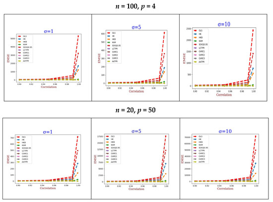
Figure 2. Graphical display of Table 2.

Figure 3. Graphical display of Table 3.

4. Simulation Result Discussion

Our comprehensive simulation studies yield the following significant findings:

• Superior Performance of AATPR:

The proposed AATPR estimator consistently outperforms all competing ridge estimators in terms of minimum mean squared error (MSE) across all simulated scenarios. This superior performance persists regardless of sample size, error variance, or number of predictors. As expected, the OLS estimator demonstrates the least robustness to multicollinearity, consistent with previous findings [2,18,20].

2.

Robustness Against Multicollinearity:

Figure 1, Figure 2 and Figure 3 (derived from Table 1, Table 2 and Table 3) clearly demonstrate that while MSE values for OLS and existing ridge estimators increase with rising multicollinearity [14,18,19,30], our AATPR estimator shows an inverse relationship. This remarkable performance stems from the estimator’s dynamic ability to automatically adapt its penalty structure in response to varying levels of predictor correlation.

3.

Stability Across Error Variance Levels:

Simulation results confirm a strong positive association between error variance and MSE for most estimators. However, AATPR maintains exceptional stability, showing only marginal MSE increases even under high error variance conditions combined with multicollinearity.

4.

Dimensionality Effects:

As model complexity increases (particularly in the presence of multicollinearity), all estimators exhibit rising MSE values. However, OLS shows particularly rapid deterioration compared to ridge-type estimators, aligning with established literature [30,31].

5.

Sample Size Considerations:

In compliance with general property, increasing the sample size improves estimation accuracy for all methods. However, ridge estimators (including AATPR) demonstrate consistently better performance than OLS across all sample sizes, corroborating previous findings [20].

5. Applications

To demonstrate the real-world applications of our proposed estimators and methodology, we considered two published data sets manufacturing sector data set adopted by [32] and the Pakistan GDP Growth data set [24]. These data sets possess similar features that were considered earlier in our simulation work.

5.1. Analysis of Manufacturing Sector Data

The data set contains 31 observations using three predictor variables, in the period from 1960 to 1990, considering the following regression model:

$$y={𝛶}_0+{𝛶}_1{m}_1+{𝛶}_2{m}_2+{𝛶}_3{m}_3+{ϵ}_i$$

(26)

In model (26), the response variable (y) shows the product value in the manufacturing sector, m₁ represents the values of the imported intermediate commodities, m₂ is the imported capital commodities, and m₃ is the value of imported raw materials. The eigen values of the $M^{\prime }M$ matrix are 2.9851, 0.00989, and 0.0050, respectively. The condition number is computed as 600.2598. Similarly, the variance inflation factor (VIF) for all the predictors is significantly greater than 10, i.e., for m₁, m₂, and m₃, the VIFs computed are 128.2639, 103.4284, and 70.8708. The pair-wise correlation amongst the predictors is provided in Figure 4. All these indicate a severe multicollinearity problem in the data.

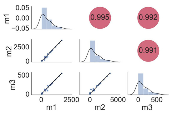
Figure 4. Pair-wise correlation for manufacturing sector data.

The EMSE and regression coefficients of all the considered estimators are given in Table 4. The results revealed that all the ridge estimators performed much better compared to OLS, as reported by [14,20]. The proposed estimator AATPR recorded the minimum MSE amongst all the considered estimators. Moreover, as mentioned by [33], multicollinearity may cause the regression coefficients of OLS to alter their signs; in our case, this happens with ${𝛶}_1$ and ${𝛶}_2$.

Table 4. EMSE and regression coefficients of manufacturing sector data.

Estimators	OLS	HK	HKB	KAM	SCKQ0.95	LCTPR	TKTPR	CARE1	CARE2	CARE3	AATPR
Amount of biasedness	-	0.09	0.04	0.05	0.08	0.03	3.89	25.07	1258.76	18,464.79	44.46
MSE	3.484	0.501	0.469	0.475	0.498	0.480	6.308	0.824	0.885	0.887	0.215
${𝛶}_1$	0.2079	−0.5738	−0.5741	−0.5740	−0.5738	−0.5745	−0.5741	−0.5743	−0.5743	−0.5743	−0.5743
${𝛶}_2$	0.9205	−0.5169	−0.5915	−0.5727	−0.5239	−0.6142	0.0527	−0.0100	−0.0024	−0.0022	−0.0022
${𝛶}_3$	−0.134	−0.2314	−0.2911	−0.2750	−0.2366	−0.3116	0.0139	−0.0028	−0.0007	−0.0006	−0.0006

5.2. Analysis of Pakistan GDP Growth Data

This data set contains data for the financial years 2008 to 2021, considering the linear regression model as follows:

$$y={𝛶}_0+{𝛶}_1{m}_1+{𝛶}_2{m}_2+{𝛶}_3{m}_3+{𝛶}_4{m}_4+{𝛶}_5{m}_5+{𝛶}_6{m}_6+{𝛶}_7{m}_7+{𝛶}_8{m}_8+{ϵ}_i$$

(27)

In model (27), “y” is the GDP rate, m₁ is milk production, m₂ is meat production, m₃ is the number of Buffalo, m₄ is the number of Cattle, m₅ is the number of Poultry, m₆ is Consumer Price Index, m₇ is tax to GDP ratio, and m₈ is investment to GDP ratio. The eigen values, of the $M^{\prime }M$ matrix are 6.04, 1.13, 0.74, 0.08, 0.0018, 0.00003, 0.000004, and 0.000001, respectively. The condition number is computed as 5,210,223. Similarly, the variance inflation factor (VIF) for most of the predictors is significantly greater than 10, i.e., for m₁, m₂, m₃, m₄, m₅, m₆, m₇, and m₈, the VIFs computed are 132,350, 633,144, 21,894, 194,158, 144,521, 6, 32, and 8. The pair-wise correlation amongst the predictors is provided in Figure 5. All these indicate a severe multicollinearity problem in the data. The EMSE and regression coefficients for Pakistan DGP Growth Data are given in Table 5.

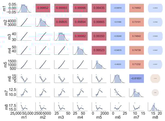
Figure 5. Pair-wise correlation for Pakistan DGP Growth Data.

Table 5. EMSE and regression coefficients of Pakistan GDP Growth Data.

Estimators	OLS	HK	HKB	KAM	SCKQ0.95	LCTPR	TKTPR	CARE1	CARE2	CARE3	AATPR
Amount of biasedness	-	0.08	0.06	437.08	2265.26	0.01	1.61	2282.73	10,421,695.90	11,898.13	5.89
MSE	1,343,764	17,916.52	15,019.98	14,639.78	14,639.79	17,962.52	14,645.46	14,639.76	14,639.76	14,639.76	14,139.21
${𝛶}_1$	−48.1081	−0.0185	−0.0185	−0.0028	−0.0006	−0.0186	−0.0136	−0.0994	−0.1015	−0.1015	−0.1291
${𝛶}_2$	100.2213	−0.4462	−0.4462	−0.0145	−0.0029	−0.4492	−0.3602	−0.4605	−0.4573	−0.4573	−0.6795
${𝛶}_3$	−3.1256	0.5814	0.5814	0.0126	0.0025	0.5852	0.5014	0.3955	0.3918	0.3918	0.4053
${𝛶}_4$	−2.5076	0.4883	0.4880	0.0012	0.0002	0.4914	−0.6805	0.0367	0.0362	0.0362	0.3600
${𝛶}_5$	−47.5806	3.4464	3.3672	0.0002	0.0000	3.4688	−0.0373	0.0058	0.0058	0.0058	0.0061
${𝛶}_6$	−0.9127	−1.7387	−0.7667	0.0000	0.0000	−1.7500	0.0003	−0.0001	−0.0001	−0.0001	−0.0333
${𝛶}_7$	0.4716	−14.1422	−2.9307	0.0000	0.0000	−14.2342	0.0009	−0.0001	−0.0001	−0.0001	−0.0181
${𝛶}_8$	−0.2461	16.6068	2.6074	0.0000	0.0000	16.7149	−0.0008	0.0001	0.0001	0.0001	0.1644

6. Conclusions

In this paper, we propose an auto-tuning two-parameter ridge (AATPR) estimator that dynamically adjusts shrinkage parameters in response to the condition number of the design matrix (multicollinearity), model dimensionality, and error variance. The estimator’s adaptive mechanism optimizes the bias–variance tradeoff, yielding superior performance compared to existing ridge methods as demonstrated through Monte Carlo simulations and empirical applications. Potential extensions to models with concurrent multicollinearity and heteroscedasticity are identified as valuable future research directions.

References

- Lipovetsky, S.; Conklin, W.M. Ridge regression in two-parameter solution. Appl. Stoch. Models Bus. Ind. 2005, 21, 525–540. [Google Scholar] [CrossRef]
- Khan, M.S.; Ali, A.; Suhail, M.; Alotaibi, E.S.; Alsubaie, N.E. On the estimation of ridge penalty in linear regression: Simulation and application. Kuwait J. Sci. 2024, 51, 100273. [Google Scholar] [CrossRef]
- Hoerl, A.E.; Kennard, R.W. Ridge Regression: Biased Estimation for Nonorthogonal Problems. Technometrics 1970, 42, 80. [Google Scholar]
- Hoerl, A.E.; Kennard, R.W. Ridge Regression: Applications to Nonorthogonal Problems. Technometrics 1970, 12, 69. [Google Scholar] [CrossRef]
- Massy, W.F. Principal Components Regression in Exploratory Statistical Research. J. Am. Stat. Assoc. 1965, 60, 234–256. [Google Scholar] [CrossRef]
- Zou, H.; Trevor, H. Regularization and Variable Selection Via the Elastic Net. J. R. Stat. Soc. Ser. B Stat. Methodol. 2005, 67, 301–320. [Google Scholar] [CrossRef]
- Garcia, C.G.; Pérez, J.G.; Liria, J.S. The raise method. An alternative procedure to estimate the parameters in presence of collinearity. Qual. Quant. 2011, 45, 403–423. [Google Scholar] [CrossRef]
- Garcia, C.B.; Salmeron, R.; Claudia, G.; Jose, G. Residualization: Justification, Properties and Application. J. Appl. Stat. 2020, 47, 1990–2010. [Google Scholar] [CrossRef]
- Belsley, D. A Guide to Using the Collinearity Diagnostics. Comput. Sci. Econ. Manag. 1991, 4, 33–50. [Google Scholar] [CrossRef]
- Dar, I.S.; Chand, S. Bootstrap-quantile ridge estimator for linear regression with applications. PLoS ONE 2024, 19, e0302221. [Google Scholar] [CrossRef]
- McDonald, G.C. Ridge Regression. Wiley Interdiscip. Rev. Comput. Stat. 2009, 1, 93–100. [Google Scholar] [CrossRef]
- Hocking, R.R.; Speed, F.M.; Lynn, M.J. American Society for Quality A Class of Biased Estimators in Linear Regression. Technometrics 1976, 18, 425–437. [Google Scholar] [CrossRef]
- Hoerl, A.E.; Kannard, R.W.; Baldwin, K.F. Ridge regression: Some simulations. Commun. Stat. 1975, 4, 105–123. [Google Scholar] [CrossRef]
- Suhail, M.; Chand, S.; Kibria, B.M.G. Quantile based estimation of biasing parameters in ridge regression model. Commun. Stat. Simul. Comput. 2020, 49, 2732–2744. [Google Scholar] [CrossRef]
- Lipovetsky, S. Two-parameter ridge regression and its convergence to the eventual pairwise model. Math. Comput. Model. 2006, 44, 304–318. [Google Scholar] [CrossRef]
- Toker, S.; Kaçiranlar, S. On the performance of two parameter ridge estimator under the mean square error criterion. Appl. Math. Comput. 2013, 219, 4718–4728. [Google Scholar] [CrossRef]
- Kuran, Ö.; Özbay, N. Improving prediction by means of a two parameter approach in linear mixed models. J. Stat. Comput. Simul. 2021, 91, 3721–3743. [Google Scholar] [CrossRef]
- Akhtar, N.; Alharthi, M.F. Enhancing accuracy in modelling highly multicollinear data using alternative shrinkage parameters for ridge regression methods. Sci. Rep. 2025, 15, 10774. [Google Scholar] [CrossRef]
- Alharthi, M.F.; Akhtar, N. Newly Improved Two-Parameter Ridge Estimators: A Better Approach for Mitigating Multicollinearity in Regression Analysis. Axioms 2025, 14, 186. [Google Scholar] [CrossRef]
- Kibria, B.M.G. Performance of some New Ridge regression estimators. Commun. Stat. Part B Simul. Comput. 2003, 32, 419–435. [Google Scholar] [CrossRef]
- Khalaf, G.; Mansson, K.; Shukur, G. Modified ridge regression estimators. Commun. Stat. Theory Methods 2013, 42, 1476–1487. [Google Scholar] [CrossRef]
- Sengupta, N.; Sowell, F. On the Asymptotic Distribution of Ridge Regression Estimators Using Training and Test Samples. Econometrics 2020, 8, 39. [Google Scholar] [CrossRef]
- Cochran, W.G. Sampling Techniques; John Wiley & Sons: Hoboken, NJ, USA, 2007. [Google Scholar]
- Khan, M.S.; Ali, A.; Suhail, M.; Awwad, F.A.; Ismail, E.A.A.; Ahmad, H. On the performance of two-parameter ridge estimators for handling multicollinearity problem in linear regression: Simulation and application. AIP Adv. 2023, 13, 115208. Available online: https://pubs.aip.org/adv/article/13/11/115208/2920711/On-the-performance-of-two-parameter-ridge (accessed on 2 September 2025). [CrossRef]
- Haq, M.S.; Kibira, B.M.G. A Shrinkage Estimator for the Restricted Linear Regression Model: Ridge Regression Approach. J. Appl. Stat. Sci. 1996, 3, 301–316. [Google Scholar]
- Mcdonald, G.C.; Galarneau, D.I.; Galarneau, D.I. A Monte Carlo Evaluation of Some Ridge-Type Estimators. J. Am. Stat. Assoc. 1975, 70, 407–416. [Google Scholar] [CrossRef]
- Suhail, M.; Chand, S.; Aslam, M. New quantile based ridge M-estimator for linear regression models with multicollinearity and outliers. Commun. Stat. Simul. Comput. 2021, 52, 1417–1434. [Google Scholar] [CrossRef]
- Halawa, A.M.; El Bassiouni, M.Y. Tests of regression coefficients under ridge regression models. J. Stat. Comput. Simul. 2000, 65, 341–356. [Google Scholar] [CrossRef]
- Newhouse, J.P.; Oman, S.D. An Evaluation of Ridge Estimators; Rand Corporation: Santa Monica, CA, USA, 1971; 716p. [Google Scholar]
- Yasin, S.; Kamal, S.; Suhail, M. Performance of Some New Ridge Parameters in Two-Parameter Ridge Regression Model. Iran. J. Sci. Technol. Trans. A Sci. 2021, 45, 327–341. [Google Scholar] [CrossRef]
- Majid, A.; Ahmad, S.; Aslam, M.; Kashif, M. A robust Kibria–Lukman estimator for linear regression model to combat multicollinearity and outliers. Concurr. Comput. 2022, 35, e7533. [Google Scholar] [CrossRef]
- Eledum, H.; Zahri, M. RELAXATION METHOD FOR TWO STAGES RIDGE REGRESSION ESTIMATOR. Int. J. Pure Appl. Math. 2013, 85, 653–667. [Google Scholar] [CrossRef]
- Gujarati, D.N.; Porter, D.C. Basic Econometrics, 5th ed.; McGraw Hill: Columbus, OH, USA, 2009. [Google Scholar]
Disclaimer/Publisher’s Note: The statements, opinions and data contained in all publications are solely those of the individual author(s) and contributor(s) and not of MDPI and/or the editor(s). MDPI and/or the editor(s) disclaim responsibility for any injury to people or property resulting from any ideas, methods, instructions or products referred to in the content. |
© 2025 by the authors. Licensee MDPI, Basel, Switzerland. This article is an open access article distributed under the terms and conditions of the Creative Commons Attribution (CC BY) license (https://creativecommons.org/licenses/by/4.0/).