Abstract
In this paper, we address the problem of increasing the number of regenerations in the simulation of the workload process in a single-server queueing system. To this end, we extend the splitting technique developed for the Markov workload process in the M/M/1 queue to the more general GI/M/1 queueing systems. This approach is based on a minorization condition for the transition kernel of the workload process, which is a Markov chain defined by the Lindley recursion. The proposed method increases the number of regenerations during the simulation and potentially reduces the time required to estimate stationary performance metrics with a given level of precision.
MSC:
94-10
1. Introduction
Estimating stationary performance in non-Markovian queueing systems is, as a rule, a challenging problem. The regenerative approach offers a powerful method for addressing this issue when the underlying stochastic process that describes the dynamics of the model possesses the regeneration property. In such cases, the process trajectory can be decomposed into independent and identically distributed (i.i.d.) cycles, and the estimation relies on the regenerative version of the Central Limit Theorem (CLT), where the independence of cycles plays a key role. The frequency of regeneration points separating these cycles is crucial for simulation efficiency: the fewer the number of regeneration times, the longer the simulation must run to obtain an estimate with a given level of precision. This is analogous to the classical setting involving i.i.d. data, where more observations are needed for more accurate estimation. In the regenerative setting, each simulated regeneration cycle contributes as a data point, obtained by summing the values of the process over that cycle.
Analogously to the classical case, the regenerative approach encounters difficulties when the number of regenerations grows very slowly during the simulation. This can result in unacceptably long simulation times being required to obtain the desired estimates. In such situations, speed-up simulation techniques (particularly those that increase the frequency of regeneration points) are highly desirable. Significant progress in constructing regenerations for the so-called Harris Markov chains (with general state spaces) has been made in the foundational papers [1,2]. The approach developed in these works is primarily of theoretical importance, enabling, in particular, proof of the existence of stationary regimes in the stochastic models under consideration. Related developments can be found in [3,4].
The key idea introduced in [1,2] is that, for a broad class of Markov chains, it is possible to construct so-called one-dependent regeneration cycles. In this setting, while adjacent cycles may be dependent, the regeneration times themselves form a renewal process, that is, the lengths of the regeneration cycles are i.i.d. In other words, such chains possess a hidden regenerative structure that, however, becomes apparent only after a suitable randomization.
More specifically, this randomization arises from the minorization condition satisfied by the transition kernel. Under this condition, once the Markov chain enters a certain set, its subsequent path, with a fixed probability, starts independently of the previous state, thus inducing a randomized (artificial) regeneration. The splitting procedure based on this minorization condition is a key tool in this analysis. Previously, artificial regeneration based on the exponential splitting technique was applied by the authors to the study of a single-server queueing system with a superposed input process formed by independent stationary renewal processes [5,6].
As mentioned above, this approach has been widely and successfully employed in the theoretical analysis of Harris Markov chains. However, its practical application often faces significant challenges, particularly in the recovering a part of the trajectory after identifying randomized regeneration points during simulation (see the discussion in [7] and also Chapter VII of [8] for more information on this issue).
To partially overcome this difficulty, a practical implementation was proposed in [7]. This method enables a feasible application of the splitting technique in simulation. Specifically, ref. [7] demonstrates this by conducting a splitting-based regenerative analysis of the stationary workload process in the well-known queue. Furthermore, as shown in [7], in some cases the construction of more frequent regeneration points also leads to a reduction in the asymptotic variane of the CLT-based confidence interval estimators. Namely, it was proved in [7] that if one sequence of regenerations is a superset of another sequence of regenerations, then the superset provides a smaller asymptotic variance of the regenerative variance estimator. A number of works are devoted to the influence of the choice of the regeneration state on the time-average variance constant (TAVC) and asymptotic variance, such as [9,10,11,12]. In [12], the authors study systems in which interarrival times follow distributions with exponential or heavier tails, allowing a decomposition that includes an exponential component (in fact, this decomposition is similar to exponential splitting). This decomposition is used to construct an embedded sequence of regeneration times. Through numerical simulations, they demonstrate that choosing the exponential component with the largest mean minimizes the asymptotic variance of the standard deviation estimator for the performance measure. In [9], a set of examples demonstrating the influence of the regeneration state for a TAVC queue process in systems is discussed.
In the present paper, we extend the approach of [7] to a more general queueing system: the queue with specific renewal input processes. This constitutes the main theoretical contribution of our work. In particular, we extend the analysis to include systems with hyperexponential and Pareto interarrival time distributions. We emphasize that applying the minorization condition is a nontrivial task, as it depends on the form of the underlying interarrival time distribution. Specifically, it requires the construction and implementation of the “residual” distribution that arises in the analysis of the minorization condition (see, for example, Formula (3) below). In more detail, we first provide a comprehensive analysis of the system, addressing several aspects that were omitted in [7]. We then extend the method to cases with and Pareto interarrival distributions. Next, we conduct simulations to record the number of regenerations generated through the splitting technique and use the regenerative CLT to construct confidence intervals for some performance metrics related to the steady-state workload in the systems under consideration.
The paper’s second major contribution is a numerical analysis comparing classical regeneration cycles with those based on randomized (splitting-induced) regenerations, along with their respective estimators. We note that the terms “randomized”,“splitting-based”, and “artificial” are used interchangeably throughout the paper to refer to regenerations constructed via the minorization condition.
The paper is organized as follows: Section 2, drawing primarily on [7], outlines the core constructions underlying the method. In Section 3, we examine in detail the artificial regeneration scheme for the stationary workload process in the classical system. Then, in Section 4, the analysis is extended to the model with hyperexponential interarrival times, and in Section 5, to a system with Pareto interarrival time distribution. Finally, Section 6 presents the corresponding numerical results, highlighting the frequency of both classical and randomized regenerations, along with the associated confidence estimates.
2. Minorization and Artificial Regeneration
Although the focus of this paper is on queueing systems, we begin by briefly discussing the randomized regeneration of a general time-homogeneous Markov chain , defined on a measurable space with the initial state . (We assume that the -algebra is generated by a countable family of subsets of .) The one-step transition kernel is defined as
- Assume that for some set , and for every and , there are and a probabilistic measure on such that the following minorization condition holds:
- The set and the quantity are called the regeneration set and regeneration measure, respectively [13]. A key implication of condition (1) is that, after visiting the set , the chain with probability has (on the next step) the distribution , which is independent of the state x at the previous step. This event corresponds to a randomized (or artificial) regeneration of the chain [7,14].
Moreover, condition (1) enables the following mixture decomposition of the transition kernel:
where
According to representation (2), the Markov chain can be modeled using the following splitting procedure. Let be a Bernoulli random variable with parameter . If the chain is in state and , then the next state is drawn from the distribution ; otherwise, it is drawn from the distribution .
Assume that the Markov chain has a stationary distribution , and let denote the number of artificial regenerations in the interval . It is known [7] that, as ,
where is the stationary distribution of the chain Z. Thus, represents the asymptotic rate of artificial regenerations produced by the splitting mechanism.
Remark 1.
The idea of splitting the kernel of a Markov chain defined on a general state space was introduced in [1,2] to construct regenerations for so-called Harris Markov chains, which generally do not admit a single-point set satisfying the minorization condition (1). If such a set does exist, then the chain exhibits classical regenerations [8]. This latter case applies to all the scenarios considered in the present study.
In the analysis below, we consider the workload process in FIFO (First In First Out) queueing systems. This process forms a Markov chain governed by the Lindley recursion:
where , is a sequence of i.i.d. exponential service times with rate , and is a sequence of i.i.d. interarrival times with distribution function (d.f.) and mean (to denote the generic element of an i.i.d. sequence, we suppress the serial index). Let , so that ; under this condition, the workload process is stable. Moreover, the workload process is a positive recurrent regenerative process. This implies the existence of a classical regeneration structure: specifically, regenerations occur whenever an arriving customer finds the server idle, and the expected time between such regenerations is finite. In our setting, the process is classically regenerative. A key question that we address is how the rate of classical regenerations compares to the rate of randomized regenerations obtained through the splitting and minorization condition (1). More precisely, we investigate how to maximize the number of randomized regenerations of the workload process as defined by Equation (5).
In Section 3, Section 4 and Section 5, we demonstrate how to determine the regeneration rate that maximizes the number of regenerations of the workload process in certain queueing systems operating under the FIFO discipline.
2.1. Embedded Markov Chain Approach
Although the primary focus of our research is to develop randomized regeneration techniques for the continuous-time workload process beyond the classical queueing system, it is both natural and instructive to briefly consider an alternative, well-known discrete-time setting. This alternative is based on the embedded Markov chain formed by the corresponding queue-length process [8]. Let denote the arrival times of customers. Define as the number of customers in the system at time . Although the process is not Markovian, it is well-known (and straightforward to verify) that the sequence , representing the queue size just before the nth arrival, forms an irreducible, aperiodic, countable Markov chain on the state space . Each return of this chain to a given state k, i.e., an occurrence of for some l, defines a regeneration point, which we refer to (for convenience) as a k-regeneration.
Thus, such a chain regenerates at each step generating, in general, different types of (classical) regeneration. It accumulates in parallel with these regenerations and forsm different sequences of the regeneration cycles, which in turn, can be used jointly in the confidence (regenerative) estimation. Assume that is the unique solution to the equation
(For further details, see Section 5 in Chapter X of [8].) It is also well-known that, under the stability condition , the Markov chain has a stationary distribution as , given by
In particular, the frequency of 0-regenerations is given by , while the total frequency of non-zero regenerations is . It follows that if , the frequency of 0-regenerations exceeds the combined frequency of all non-zero regenerations. Conversely, if , the frequency of non-zero regenerations surpasses that of 0-regenerations, but by no more than a factor of two. This simple analysis suggests a potential advantage of using splitting-based (artificial) regenerations, even in the study of continuous-time queueing processes.
Remark 2.
To avoid misunderstanding, it is worth emphasizing that in a queueing system, if the mean service time satisfies (or, equivalently, ), then the system is stable, and the frequency of 0-regenerations approaches , while the fraction of idle server time approaches ( in queues).
Remark 3.
For the embedded Markov chain discussed above, the one-step transition from a fixed state is only possible to the states , with transition probabilities
The corresponding conditional distribution does not satisfy a (suitably modified) version of the minorization condition (2). As a result, we cannot apply all the different accumulated k-regenerations from a single simulation run to construct a confidence interval using the CLT. This stands in contrast to the case of randomized regenerations based on condition (1), as we demonstrate in Section 6.1 below.
3. Artificial Regeneration in Queueing Systems
In this section, we present a detailed construction for the system, as this analysis is extensively used in the examples that follow. Assume that the interarrival times and the service times are i.i.d. exponential r.v.s with parameter and , respectively. It is shown in [7] that for the sequence of waiting times in the system, the frequency of classical regenerations, as the simulation/observation time increases, approaches . On the other hand, ref. [7] also shows that the frequency of artificial regenerations in the system (obtained by the splitting method described in the previous section) approaches . Thus, the ratio between these two regeneration frequencies is
indicating that the number of randomized regenerations can exceed the number of classical regenerations by a factor of up to 2 as . A similar result holds for the embedded Markov chain discussed in Section 2.1.
Now, we provide proof of the limiting result , doing so to extend, in the subsequent sections, the splitting method to queuing systems with a more general renewal input process (details of this proof are not given in [7]). Using the Lindley recursion (5), we can readily derive that
and
Differentiating the conditional d.f. with respect to y yields
Now, we define
For each x, the optimal value of the splitting factor , which yields the maximal regeneration rate, is defined as (see [7])
We calculate
Furthermore, observe that
Hence, in our case, (7) simplifies to
Note that and as . Next, using the well-known stationary distribution of the workload process (which, in this system, coincides with the waiting time)
so we find that (which also equals due to the PASTA property, as shown in Remark 2 above). The corresponding stationary density function is
Using this, we can compute the regeneration rate under the randomized splitting scheme, as shown in [7]
Finally, it is also easy to find the distribution
for .
4. Artificial Regeneration in Queueing Systems
We now construct the randomized regeneration scheme for the workload process in an system, where the interarrival time distribution is hyperexponential:
It is straightforward to verify that the stability condition for this system takes the form
As in the previous section, we calculate
and
The density of the latter conditional d.f. (with respect to y), for , is
Define
then, we obtain
It then follows that, for ,
and for ,
Since the derivative of the function with respect to y (for ) is given by
then is decreasing in y. Therefore, . Hence, the optimal splitting factor becomes
and
Let be the stationary waiting time in a general queue. It is known that (see, e.g., [15,16])
where is the unique root of the equation
and is the Laplace–Stiltjes transform of the d.f. A. Substituting into the r.h.s. of Formula (4)
we obtain
Thus, the below statement holds.
Lemma 1.
In the queueing system, the frequency of classical regenerations is no greater than that of randomized regenerations, i.e.,
This inequality quantifies the benefit of randomized regeneration. The advantage factor—that is, the ratio of the frequencies of randomized to classical regenerations—is given by
5. Artificial Regeneration in Queueing Systems
Consider the queue, where the interarrival times are i.i.d. with Pareto distribution
and the service times are i.i.d. and exponentially distributed with rate . Assume that the stability condition holds, i.e.,
For such a system, we determine the optimal splitting factor (as a function of x) and compute the frequency of randomized regenerations using the splitting method.
Consider the sequence of waiting times and calculate the conditional probability as follows:
Let us make the substitution , so that . Substituting into the last integral, we obtain
where denotes the incomplete upper Gamma-function,
For ,
Let us make the substitution , so that . Substituting into the last integral in (11), we rewrite the final line as
Therefore, for ,
Similarly, for , we find that
Now, changing variables using , so that , we obtain
and, thus, for , the conditional d.f. equals
Putting both cases together, for all , the conditional d.f. is given by
and the corresponding density function is
Now, we determine the optimal value
Let
Then,
Furthermore, for all , it is easy to see that
Similarly, for , we find
Hence
Next, we substitute the resulting and Equation (10) into the integral (4) as follows:
We now carry out a change in variables. Let
and let
Substituting into Equation (13), we obtain
Thus, the frequency of artificial regenerations (in the limit) satisfies
Figure 1 shows the ratio of artificial to classical regeneration frequencies as a function of the parameter for the queueing system with parameters , , and . The ratio at a fixed value of increases with . For instance, when , the ratio is , , , and for and , respectively. Across all values of and considered, the artificial regeneration frequency is at least 1.37 times greater than the classical frequency, with the difference being most pronounced for small values of .
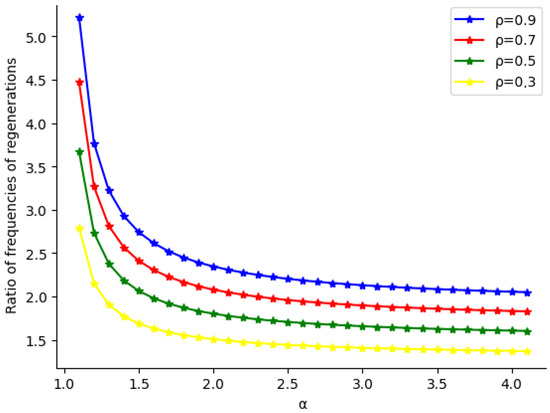
Figure 1.
A graphical comparison of artificial and classical regeneration frequencies—the ratio as a function of the parameter .
6. Simulation Results
In this section, we present simulation results for the systems discussed above. We compare the number of classical regenerations, denoted by , with the number of artificial regenerations, denoted by , across various values of traffic intensity. Let denote the i-th regeneration point, and then is the length of the i-th regeneration cycle, , where N is the number of regeneration cycles.
To identify randomized regenerations, we apply the following procedure (for n customers), following the approach outlined in [10]:
- 1.
- Compute using Lindley’s recursion:
- 2.
- Set and compute the quantities , and .
- 3.
- Generate a Bernoulli r.v. with success probabilityIf , then is a regeneration time: set with and increment .
- 4.
- Repeat steps 1–3 for until .
Table 1 presents the simulation results for the system with , , and various values of . As observed, the simulation results are in good agreement with the theoretical expectations. Specifically, the frequency of classical regenerations, , aligns with the theoretical probability of classical regeneration, , while the frequency of artificial regenerations, , closely matches the theoretical frequency . For example, when , the frequency of classical regenerations is , and the frequency of artificial regenerations is , which is close to .

Table 1.
Number of regenerations in queues.
Table 2 refers to queueing systems with , , , , and various values of . As observed, the simulation results are in good agreement with the theoretical predictions. Specifically, the frequency of classical regenerations, , corresponds to the theoretical probability of classical regeneration, , while the frequency of artificial regenerations, , closely matches the theoretical probability of artificial regeneration, . Furthermore, for , the number of artificial regenerations, , is approximately twice the number of classical regenerations, .
Table 2.
Number of regenerations in queues.
Table 3 presents the simulation results for the system with , , , and various values of . As in the previous example, for , the number of artificial regenerations, , is approximately twice that of classical regenerations. It is also worth noting that the empirical frequencies of both classical and artificial regenerations closely match their respective theoretical probabilities.
Table 3.
Number of regenerations in queues with and .
Now, we fix and vary the service rate to explore different values of . Table 4 highlights that the number of randomized regenerations exceeds that of classical regenerations for . It is worth noting that, in this case, the overall number of regenerations (both classical and randomized) is relatively low for the same values of traffic intensity due to the small value of . However, the number of observed regenerations remains sufficient for reliable evaluation.
Table 4.
Number of regenerations in queues with and .
6.1. On Confidence Estimation
Regenerations (both classical and randomized) can be used in the standard way to construct a confidence interval for a target performance measure of the stationary process X, where f is a measurable function. This approach relies on the well-known ratio formula for regenerative processes. In the discrete-time setting, for a regenerative process , the expectation is given by
where is the generic regeneration cycle length. In this representation, denotes the expectation given that X has distribution at the beginning of a regeneration cycle. In our study, we simulate the workload process using the Lindley recursion (5) in such a way that the initial value at the beginning of each regeneration cycle is distributed according to .
Recall that the estimation of is based on the convergence (below, for simplicity, we omit the symbol in the definition of the expectation ) [7,17]
where is the time-average variance constant,
and are estimates of and , respectively, and .
The regenerative version of the CLT gives the following confidence interval for r [11]:
where and
is an estimator of the TAVC . To assess the efficiency of the estimator , the CLT for the standard deviation can be applied (see [9]):
where
and
Table 5 presents simulation results for the confidence estimation of the stationary waiting time W in the system with and . Here, is the theoretical mean of W, is the empirical mean estimate based on classical regeneration, and is the empirical mean estimate based on artificial regeneration. Similarly, and represent the half-width of the corresponding 95% confidence interval (15) computed using classical and artificial regeneration, respectively. The results show that both regeneration methods yield similar estimates, indicating that the choice of regeneration method does not affect the accuracy of the performance measure.
Table 5.
Confidence estimations of W in queues.
The regeneration cycle lengths for both types of regeneration, along with the corresponding estimates of and , are presented in Table 6 for the system with and various values of , using samples. We denote by () the mean cycle length under classical (artificial) regeneration. Similarly, and (, ) denote the estimates of and obtained via classical (artificial) regeneration.
Table 6.
Regeneration in queues with and .
As observed, for relatively small values of , randomized regeneration offers a significant advantage in terms of confidence interval width. For example, when , the mean classical regeneration cycle length is approximately 364, implying that only about 27 cycles are expected for customers. This raises concerns about the reliability of estimates based on the regenerative CLT. In contrast, randomized regeneration yields approximately 81 cycles under the same conditions. The simulation results further indicate that the TAVC is independent of the regeneration type, whereas the asymptotic variance is smaller when artificial regeneration is employed.
Let denote the number of customers in the queue at time . Using the regenerative simulation technique, we estimate the joint probability that two events occur simultaneously: the waiting time W exceeds a given high threshold , and the queue length Q exceeds another threshold .
Table 7 presents simulation results for estimating in the system with , , , , and . For this system, no analytical expression for this probability is available. We denote by the theoretical value of and by and the corresponding estimates of obtained using classical and artificial regeneration, respectively. Similarly, and denote the estimates of .
Table 7.
Estimation of in queues for .
It is worth noting that the estimates of and are invariant with respect to the type of regeneration. Since no analytical expressions are available for these probabilities, regenerative simulation provides a viable method for obtaining their estimates.
In summary, as demonstrated above, randomized regeneration offers advantages in simulation-based estimation in scenarios where the classical approach is less effective.
7. Conclusions
In this paper, the splitting method, originally proposed in [7] to accelerate regenerations of the workload process, is extended to a broader class of stationary systems with renewal input processes featuring hyperexponential and Pareto interarrival time distributions. The effectiveness of the method is demonstrated through numerical examples, which highlight scenarios where randomized regeneration outperforms classical regeneration. In such cases, the limiting estimates obtained using both types of regeneration are close, but the use of randomized regeneration significantly reduces the simulation time required to construct confidence intervals based on the regenerative CLT. The considered method can be developed for systems in which the distribution is known and the minorization condition (1) is satisfied.
Author Contributions
Conceptualization, I.P.; Validation, M.P.; Writing—original draft, I.P. and E.M.; Writing—review and editing, E.M. and M.P.; Supervision, E.M. and M.P.; Project administration, E.M. All authors have read and agreed to the published version of this manuscript.
Funding
This research received no external funding.
Data Availability Statement
The original contributions presented in this study are included in the article. Further inquiries can be directed to the first author.
Acknowledgments
This research was partially supported by the Italian Ministry of Education and Research (MIUR) through the framework of the FoReLab project (Departments of Excellence). During the preparation of this manuscript, the authors used ChatGPT (GPT-5, https://chatgpt.com/, accessed on 12 August 2025) for the purposes of English correction and rephrasing in some sections of the manuscript. The authors have reviewed and edited the output and take full responsibility for the content of this publication. It was not used to generate new content or ideas; it was employed only as a tool to enhance the smoothness and correctness of the existing text. The authors would like to thank anonymous referees for their helpful comments.
Conflicts of Interest
The authors declare no conflicts of interest.
Abbreviations
The following abbreviations are used in this manuscript:
| FIFO | First In First Out |
| i.i.d. | independent and identically distributed |
| r.v. | random variable |
| d.f. | distribution function |
| r.h.s | right-hand side |
| CLT | Central Limit Theorem |
| CI | confidence interval |
| w.p.1 | with probability 1 |
References
- Athreya, K.B.; Ney, P. A New Approach to the Limit Theory of Recurrent Markov Chains. Trans. Am. Math. Soc. 1978, 245, 493–501. [Google Scholar] [CrossRef]
- Nummelin, E. A Splitting Technique for Harris Recurrent Markov Chains. Z. Für Wahrscheinlichkeitstheorie Und Verwandte Geb. 1978, 43, 309–318. [Google Scholar] [CrossRef]
- Glynn, P.W. Some topics in regenerative steady-state simulation. Acta Appl. Math. 1994, 34, 225–236. [Google Scholar] [CrossRef]
- Nummelin, E. Regeneration in tandem queues. Adv. Appl. Prob. 1981, 13, 221–230. [Google Scholar] [CrossRef]
- Peshkova, I.; Morozov, E.; Pagano, M. Regenerative Analysis and Approximation of Queueing Systems with Superposed Input Processes. Mathematics 2024, 12, 2202. [Google Scholar] [CrossRef]
- Peshkova, I.; Pagano, M.; Morozov, E. Regeneration and approximation of a queueing system fed by superposed input with Weibull components. Reliab. Theory Appl. 2025, 20, 108–117. [Google Scholar] [CrossRef]
- Andradottir, S.; Calvin, M.; Glynn, P.W. Accelerated regeneration for Markov chain simulation. Probab. Eng. Inf. Sci. 1995, 9, 497–523. [Google Scholar] [CrossRef]
- Asmussen, S. Applied Probability and Queues, 2nd ed.; Springer: Berlin/Heidelberg, Germany, 2003. [Google Scholar]
- Glynn, P.W.; Iglehart, D.L. A joint central limit theorem for the sample mean and regenerative variance estimator. Ann. Oper. Res. 1987, 8, 41–55. [Google Scholar] [CrossRef]
- Glynn, P.W.; L’Ecuyer, P. Likelihood Ratio Gradient Estimation for Stochastic Recursions. Adv. Appl. Probab. 1995, 27, 1019–1053. [Google Scholar] [CrossRef][Green Version]
- Henderson, S.G.; Nelson, B.L. (Eds.) Handbook in Operations Research and Management Science: Simulation; North-Holland, Elsevier: Amsterdam, The Netherlands, 2006; Volume 13, pp. 477–500. [Google Scholar] [CrossRef]
- Moka, S.B.; Juneja, S. Regenerative simulation for queueing networks with exponential or heavier tail arrival distributions. ACM Trans. Model. Comput. Simul. (TOMACS) 2015, 25, 1–22. [Google Scholar] [CrossRef]
- Sigman, K.; Wolff, R.W. A review of regenerative processes. SIAM Rev. 1993, 35, 269–288. [Google Scholar] [CrossRef]
- Andronov, A. Artificial regeneration points for stochastic simulation of complex systems. In Simulation Technology: Science and Art, Proceedings of the 10th European Simulation Symposium, Nottingham, UK, 25–28 October 1998; SCS: Delft, The Netherlands, 1998; pp. 34–40. [Google Scholar]
- Cohen, J.W. The Single Server Queue, 2nd impression; North-Holland: Amsterdam, The Netherlands, 1992. [Google Scholar]
- Serfozo, R.F. Basics of Applied Stochastic Processes; Springer: Berlin/Heidelberg, Germany, 2009. [Google Scholar]
- Glynn, P.W.; Iglehart, D.L. Conditions for the applicability of the regenerative method. Manag. Sci. 1993, 39, 1108–1111. [Google Scholar] [CrossRef]

Disclaimer/Publisher’s Note: The statements, opinions and data contained in all publications are solely those of the individual author(s) and contributor(s) and not of MDPI and/or the editor(s). MDPI and/or the editor(s) disclaim responsibility for any injury to people or property resulting from any ideas, methods, instructions or products referred to in the content. |
© 2025 by the authors. Licensee MDPI, Basel, Switzerland. This article is an open access article distributed under the terms and conditions of the Creative Commons Attribution (CC BY) license (https://creativecommons.org/licenses/by/4.0/).