A New One-Parameter Model by Extending Maxwell–Boltzmann Theory to Discrete Lifetime Modeling

Abstract

The Maxwell–Boltzmann (MB) distribution is fundamental in statistical physics, providing an exact description of particle speed or energy distributions. In this study, a discrete formulation derived via the survival function discretization technique extends the MB model’s theoretical strengths to realistically handle lifetime and reliability data recorded in integer form, enabling accurate modeling under inherently discrete or censored observation schemes. The proposed discrete MB (DMB) model preserves the continuous MB’s flexibility in capturing diverse hazard rate shapes, while directly addressing the discrete and often censored nature of real-world lifetime and reliability data. Its formulation accommodates right-skewed, left-skewed, and symmetric probability mass functions with an inherently increasing hazard rate, enabling robust modeling of negatively skewed and monotonic-failure processes where competing discrete models underperform. We establish a comprehensive suite of distributional properties, including closed-form expressions for the probability mass, cumulative distribution, hazard functions, quantiles, raw moments, dispersion indices, and order statistics. For parameter estimation under Type-II censoring, we develop maximum likelihood, Bayesian, and bootstrap-based approaches and propose six distinct interval estimation methods encompassing frequentist, resampling, and Bayesian paradigms. Extensive Monte Carlo simulations systematically compare estimator performance across varying sample sizes, censoring levels, and prior structures, revealing the superiority of Bayesian–MCMC estimators with highest posterior density intervals in small- to moderate-sample regimes. Two genuine datasets—spanning engineering reliability and clinical survival contexts—demonstrate the DMB model’s superior goodness-of-fit and predictive accuracy over eleven competing discrete lifetime models.

1. Introduction

In recent decades, discrete distributions have been suggested as a preferable alternative to continuous distributions for complex count datasets. Classical models including binomial, Poisson, geometric, and negative binomial distributions are commonly used to model count data; however, they may not always yield the greatest fit. This highlights the need for more adaptable distribution methods. According to Alizadeh et al. [1], modeling using continuous lifespan distributions is a popular topic in a variety of sectors, including engineering science, medicine, economics, and others. Geometric and negative binomial distributions are used as discrete substitutes for the gamma and exponential distributions. However, these distributions do not always correspond to the facts as viewed. Several continuous lifespan distributions have recently been discretized in the literature due to the demand for more reliable discrete distributions capable of replicating discrete data in a range of real-world scenarios. In decision analysis, discretization refers to the process of reducing probability distributions of uncertainty to a small number of point masses that occur frequently. More information is available in Keefer and Bodily [2].

Determining the values of numerous points in the distribution, much less the actual distribution, can be difficult or costly when a decision analysis model is ambiguous. To speed up the computation and reduce the expense of computing some parallels, discretization substitutes difficult and computationally expensive integrations with the evaluation of a small number of utilities. Miller and Rice [3] discovered that discretization improves a decision analyst’s ability to communicate with clients. Even with increased processing power, discretization allows for the examination and assessment of conclusions that humans cannot understand. One way to think about the discretization process is as two separate processes. The first step is to select the points that will be used for discretization. These points typically correspond to the percentiles of the original distribution.

In the second phase of the discretization process, each location is assigned a probability mass. Days can reflect the length of life for people with brain tumors, or the period required for remission to return to survival studies. Every second of the day, reliability engineers check to see whether a system is operational. The observed data display the number of units that were completed successfully before breaking down. The count phenomenon can be observed in a variety of real-world circumstances, including accident frequency, ecological species types, insurance claims, and longevity data. Discrete distributions are effective for simulating lifespan data in certain cases. Because of their usefulness, discretization techniques are extensively used. Discrete probability distributions can be obtained by dividing them into intervals based on values or cumulative distributions. Each time, a percentile is assigned to the mean or median. Finally, each interval is allocated a probability proportional to its size. Means and percentiles are another option for discretization. Nakagawa and Osaki [4] provide information on the odds corresponding to the seconds in the original distribution.

Discrete models have recently been developed for use in domains such as medical, engineering, reliability studies, and survival analysis. For a more in-depth understanding and practical uses of discrete distributions, see references such as Alotaibi et al. [5] and Chesneau et al. [6]. While these studies expand discrete reliability theory and other application areas, they generally rely on continuous formulations or generic discretization techniques, which do not address the intricacies of the Maxwell–Boltzmann (MB) distribution. As a result, several scholars have made significant contributions to the growth of discrete dependability theory by introducing novel perspectives and approaches. Several discretization techniques are used to convert continuous models into discrete equivalents, and these techniques have been extensively studied and documented in scientific publications. The purpose of these strategies is to create discrete distributions that closely match their continuous sources. The literature has investigated several discretization strategies; Lai [7], Chakraborty [8], Afify et al. [9], and Augusto Taconeli and Rodrigues de Lara [10] are some examples.

A prominent method in the creation of discrete distributions is the use of the survival function as a discretization technique. Notable contributions in this field include the derivation of discrete analogs for the normal and Rayleigh distributions, which were presented by Roy ([11] and [12]), respectively, both of which used the survival function methodology. Building on this framework, Bebbington et al. [13] conducted a thorough investigation of the discrete additive counterpart of the Weibull distribution. Later, Haj Ahmad and Elshahhat [14], among others, provide further developments and examples of discrete transformations across different distributions.

In this study, we use the survival discretization approach to convert the continuous MB distribution into its discrete counterpart. Despite the MB distribution’s excellent adaptability in replicating various shapes of hazard rate function (HRF) in a continuous framework, real-world applications typically require data that have been censored or recorded at discrete intervals. In addition to preserving crucial statistical properties like percentiles and quantiles, discretizing the MB distribution using the survival function approach makes it easier to evaluate data that are subject to restrictions like Type-II censoring. This discrete formulation directly addresses the practical difficulties in survival and reliability analysis, which require discretely recording the exact time of failure occurrences for precise modeling and inference. Compared to traditional discretization procedures, this approach provides a framework that is more resilient to data inconsistencies while retaining the essential properties of the continuous model.

We address the limitations of the discrete MB (DMB) model, such as its computational complexity and reliance on numerical approaches, by extensive simulation tests and methodological modifications. Although our comparative study found that the DMB model performed better, it may be susceptible to certain types of data distributions, particularly if the failure rate deviates from the monotonic hazard rate structure that the model is designed to support. We assume that only the first r failure times, denoted as $y_1<y_2<\cdots <y_r$, are reported when n items undergo a life-testing experiment. This set is known as a type-II censored (T2C) sample; $\mathbf{y}=(y_1,y_2,\dots ,y_r)$. The remaining $n-r$ elements are constrained and only have failure times larger than $y_r$. The DMB model distinguishes itself from other one-, two-, and three-parameter discrete distributions by providing an increasing HRF form. The proposed model’s hazard rates make it suitable for modeling various datasets, including negatively skewed data. Other competitive models may not adequately model these probability mass shapes. The article introduces many statistical and reliability features, such as moments, probability functions, reliability, failure (or hazard) rates, and order statistics. The DMB distribution performed well in two real-world applications, outperforming eleven other discrete distribution models in the literature. The proposed parameters are estimated using maximum likelihood, Bayesian, and bootstrapping methods with T2C data. Monte Carlo simulations are used to evaluate the performance of the acquired estimators based on accuracy metrics such as the squared error, absolute bias, interval length, and coverage probability.

The remainder of the paper is organized as follows. Section 2 and Section 3 introduce the DMB distribution and present its main properties, respectively. Six interval estimation methods for the DMB parameter are examined in Section 4. Section 5 describes two approaches to parameter estimation. Section 6 reports and discusses the results of a Monte Carlo simulation study, while Section 7 analyzes two real-world datasets from engineering and clinical applications. Finally, Section 8 concludes the paper with the main findings and closing remarks.

2. New DMB Distribution

The Maxwell–Boltzmann (MB) distribution is a fundamental probability distribution in statistical physics that describes the distribution of speeds (or energies) of particles in an ideal gas at thermal equilibrium. Its mathematical formulation allows for precise modeling of the molecular speed, which is critical in deriving key physical laws such as the ideal gas law, diffusion rates, and reaction kinetics. The MB distribution’s importance extends beyond physics into areas like chemistry, atmospheric science, and even computational modeling, where it serves as a foundational tool for simulating particle-based systems and understanding statistical mechanics at a molecular level. For more discussions on the MB model, one may refer to Peckham and McNaught [15] and Rowlinson [16]. Now, we define the probability density function (say, $f(·)$) and the distribution function (say, $F(·)$) of a random variable X that follows a one-parameter MB($\alpha$) model, where $\alpha >0$ is a scale parameter, respectively, as

$$f(x;\alpha )={\displaystyle \frac{4}{\sqrt{\pi }}}{\displaystyle \frac{x^2}{\sqrt{{\alpha }^3}}}{e}^{-{\displaystyle \frac{x^2}{\alpha }}},x>0,$$

(1)

and

$$F(x;\alpha )={\Gamma }_{{\displaystyle \frac{3}{2}}}\left({\displaystyle \frac{x^2}{\alpha }}\right),$$

(2)

where ${\Gamma }_{\gamma }\left(\beta \right)={\displaystyle \frac{1}{\Gamma \left(\gamma \right)}}{\int }_0^{\beta }{y}^{\gamma -1}{e}^{-y}dy$ is the regularized lower incomplete gamma function, and $\Gamma \left(\gamma \right)={\int }_0^{\infty }{y}^{\gamma -1}{e}^{-y}dy$ is the complete gamma function. The equivalent form of the function (5) takes the following expression

$$\begin{array}{cc}\hfill F(x;\alpha )& =2\mathrm{erf}\left({\displaystyle \frac{x}{\sqrt{\alpha }}}\right)-{\displaystyle \frac{2}{\sqrt{\pi }}}{\displaystyle \frac{x}{\sqrt{\alpha }}}{e}^{-{\displaystyle \frac{x^2}{\alpha }}},\hfill \\ \hfill & =1-{\displaystyle \frac{4}{\sqrt{\pi }}}{\displaystyle \frac{1}{\sqrt{{\alpha }^3}}}\xi (x,2,\alpha ),\hfill \end{array}$$

(3)

where $\mathrm{erf}\left(\gamma \right)={\displaystyle \frac{2}{\sqrt{\pi }}}{\int }_0^{\gamma }{e}^{-y^2}dy$ is the error term, and $\xi (x,\gamma ,\alpha )={\int }_x^{\infty }{y}^{\gamma }{e}^{-{\displaystyle \frac{y^2}{\alpha }}}dy$.

The classical MB distribution is widely used to model continuous particle speeds; however, many real-world systems generate or require discrete data, such as counts or binned measurements. In various practical scenarios, the assumption of continuity may not align with the way data are observed or recorded. Introducing a discrete MB (DMB) distribution helps bridge this gap, enabling more accurate and computationally efficient modeling of discrete thermal systems and kinetic processes. Several discretization approaches exist, the most notable of which is survival function-based discretization. The surviving discretization approach is utilized to construct its counterpart, the DMB model. The probability mass function (PMF), cumulative distribution function (CDF), and other properties of the DMB model are now derived. Following Roy ([17,18]), the DMB’s PMF using survival discretization is defined as

$$\begin{array}{cc}\hfill \mathbb{P}(Y=y)& =\mathbb{S}\left(y\right)-\mathbb{S}(y+1),\hfill \\ \hfill & =\Omega (\alpha ;y)-\Omega (\alpha ;y+1),y=0,1,2,\dots ,\hfill \end{array}$$

(4)

where

$$\Omega (\alpha ;j)={\displaystyle \frac{4}{\sqrt{\pi }}}{\displaystyle \frac{1}{\sqrt{{\alpha }^3}}}\xi (j,2,\alpha ),j=y,y+1.$$

Consequently, from (4), the CDF and HRF of the newly DMB($\alpha$) model are

$$\begin{array}{cc}\hfill F\left(y\right)& =\mathbb{P}(X⩽y)\hfill \\ \hfill & =1-\mathbb{S}\left(y\right)+\mathbb{P}(X=y)\hfill \\ \hfill & =1-\Omega (\alpha ;y+1),\alpha >0,y=0,1,2,\dots ,\hfill \end{array}$$

(5)

and

$$\begin{array}{cc}\hfill h\left(y\right)& ={\displaystyle \frac{\mathbb{P}\left(y\right)}{\mathbb{S}\left(y\right)}}\hfill \\ \hfill & ={\displaystyle \frac{\Omega (\alpha ;y)-\Omega (\alpha ;y+1)}{1-\Omega (\alpha ;y)}},\alpha >0,y=0,1,2,\dots ,\hfill \end{array}$$

(6)

respectively. Upon several levels of DMB($\alpha$), Figure 1 displays various shapes of the PMF and HRF for the DMB distribution.

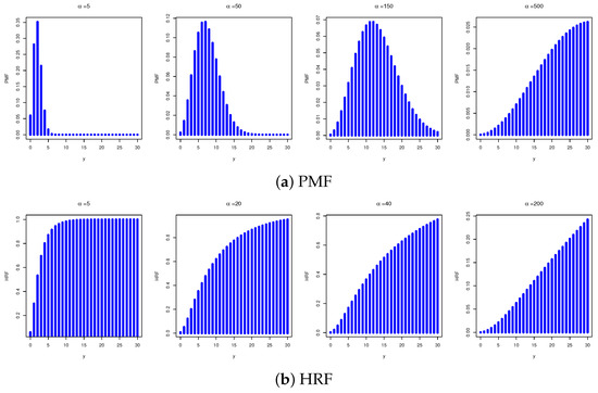
Figure 1. The PMF and HRF shapes of the new DMB distribution.

Figure 1a highlights the flexibility of the DMB’s PMF, including increasing (right-skewed), decreasing (left-skewed), or symmetrical (bell-shaped), while Figure 1b states that the DMB’s HRF is always increasing. As $\alpha$ changes, this flexibility makes the newly developed DMB highly valuable in statistical distribution theory for accurately describing a wide range of real-world discrete phenomena. In the next section, several additional statistical properties and characteristics of the DMB model, such as quantiles, moments, and ordered statistics, are derived.

Remark 1.

Krishna and Pundir [19] also proposed a discrete Maxwell distribution (dMax) obtained via SF-discretization. However, their formulation differs from ours in two important respects. First, in (4), the kernel of our distribution contains a scale factor proportional to ${\alpha }^{-3/2}$, whereas in Krishna and Pundir [19] the corresponding factor is proportional to ${\alpha }^{-1}$. For the two PMFs to coincide, both the exponential and prefactor terms would need to match. The prefactors reduce to ${\alpha }^{-3/2}\mathit{versus}{\alpha }^{-1},$ which cannot be reconciled for a free scale parameter except under a degenerate constraint. Second, this reparameterization leads to different distributional behaviors. The DMB PMF can exhibit three probability mass forms depending on the value of α (see Figure 1). By contrast, the dMax PMF in Krishna and Pundir [19] is restricted to a positively skewed shape only. This additional shape flexibility broadens the applicability of the DMB distribution, enabling it to accommodate a wider variety of empirical patterns.

3. Statistical Functions

The quantile function, moments, and order statistics are among the statistical functions for the DMB distribution that are covered in this section.

3.1. Quantiles and Moments

For a discrete distribution, the quantile function $Q\left(p\right)$ is the inverse of the CDF. It is mostly used to produce random samples for simulation purposes. To find the symbolic expression for the quantile function of the $DMB\left(\alpha \right)$ distribution, we begin with the CDF in Equation (5) and proceed algebraically as follows:

$$\begin{array}{cc}\hfill Q\left(p\right)& =F^{-1}\left(y\right)\hfill \\ \hfill & =min\left\{y\in {\mathbb{N}}_0:F\left(y\right)\ge p\right\}\hfill \\ & =\left(1-\Omega (\alpha ;y+1)\right)\ge p;\hfill \end{array}$$

hence,

$$0\le \Omega (\alpha ;y+1)\le 1-p,0<p<1,$$

(7)

where $\Omega (\alpha ;y)={\displaystyle \frac{4}{\sqrt{\pi }}}{\displaystyle \frac{1}{\sqrt{{\alpha }^3}}}\xi (y,2,\alpha )$.

Substituting $\Omega (\alpha ;y+1)$ in Equation (7), we have

$$\begin{array}{c}\hfill {\displaystyle \frac{4}{\sqrt{\alpha \pi }}}\xi (y+1,2,\alpha )\le 1-p.\end{array}$$

(8)

After some simplifications, the symbolic quantile function (8) is

$$\begin{array}{c}\hfill Q\left(p\right)=min\left\{y\in {\mathbb{N}}_0:\sum _{j=0}^y{j}^2{e}^{-j^2/\alpha }\ge p\sum _{j=0}^{\infty }{j}^2{e}^{-j^2/\alpha }\right\},0<p<1.\end{array}$$

(9)

This problem should be addressed numerically because it is based on a truncated sum of exponentially weighted quadratic terms with the denominator containing the entire infinite sum.

To calculate the moments of the DMB model, we use the non-negative random variable $y\sim DMB\left(\alpha \right)$. The following r-th is the final formula for the moment, such as ${\mu }_r^{\circ }$:

$$\begin{array}{cc}\hfill {\mu }_r^{\circ }& =\mathbb{E}\left(y^r\right)\hfill \\ \hfill & ={\displaystyle \frac{4}{\sqrt{{\alpha }^3\pi }}}\sum _{y=0}^{\infty }{y}^{r+2}{e}^{-y^2/\alpha }.\hfill \end{array}$$

(10)

With $r=1$ in Equation (10), the mean of the DMB distribution (${\mu }_1^{\circ }$) is

$$\begin{array}{cc}\hfill {\mu }_1^{\circ }& =\mathbb{E}\left(y\right)\hfill \\ \hfill & ={\displaystyle \frac{4}{\sqrt{{\alpha }^3\pi }}}\sum _{y=0}^{\infty }{y}^3{e}^{-y^2/\alpha }.\hfill \end{array}$$

(11)

To compute the variance of the DMB distribution ($\mathsf{V}$), we use the formula $\mathsf{V}={\mu }_2^{\circ }-{\left({\mu }_1^{\circ }\right)}^2$, where

$$\begin{array}{cc}\hfill {\mu }_2^{\circ }& =\mathbb{E}\left(y^2\right)\hfill \\ \hfill & ={\displaystyle \frac{4}{\sqrt{{\alpha }^3\pi }}}\sum _{y=0}^{\infty }{y}^4{e}^{-y^2/\alpha }.\hfill \end{array}$$

(12)

Using ${\mu }_i^{\circ }$ for $i=2,3,4$, the skewness, denoted by ${\Xi }_1$, and the kurtosis, denoted by ${\Xi }_2$, of the DMB distribution can be obtained, respectively, as follows:

$${\Xi }_1={\displaystyle \frac{{\mu }_3^{\circ }-3{\mu }_1^{\circ }{\mu }_2^{\circ }+2{{\mu }_1^{\circ }}^3}{{\mathsf{V}}^{1.5}}}\mathrm{and}{\Xi }_2={\displaystyle \frac{{\mu }_4^{\circ }-4{\mu }_1^{\circ }{\mu }_2^{\circ }+6{{\mu }_1^{\circ }}^2{\mu }_2^{\circ }-3{{\mu }_1^{\circ }}^4}{{\mathsf{V}}^2}}.$$

When comparing the variability of two independent samples, the coefficient of variation ($\mathsf{CV}$) is often employed, as it provides a relative measure of dispersion. The $\mathsf{CV}$ is defined as the ratio of the standard deviation to the mean and is a widely used measure of relative variability. Mathematically, it is expressed as

$$\mathsf{CV}={\displaystyle \frac{{\mathsf{V}}^{0.5}}{{\mu }_1^{\circ }}},$$

where ${\mathsf{V}}^{0.5}$ and ${\mu }_1^{\circ }$ denote the standard deviation and mean, respectively. One of the key properties of the $\mathsf{CV}$ is that it is both dimensionless and scale-invariant, making it particularly useful for comparing variability across datasets with different units or scales.

In contrast, the index of dispersion ($\mathsf{DI}$), also known as the variance-to-mean ratio, is defined as

$$\begin{array}{cc}\hfill \mathsf{DI}& ={\displaystyle \frac{\mathsf{V}}{{\mu }_1^{\circ }}}.\hfill \end{array}$$

(13)

While the $\mathsf{DI}$ is dimensionless when applied to count data or other dimensionless quantities, it is not scale-invariant. The $\mathsf{DI}$ is primarily used for non-negative discrete variables—especially count data—and plays a central role in identifying dispersion characteristics of a dataset.

The interpretation of the $\mathsf{DI}$ is as follows:

• $\mathsf{DI}>1$: indicates over-dispersion (greater variability than expected under a Poisson distribution),
• $\mathsf{DI}=1$: indicates equi-dispersion (variance equals the mean, as in the Poisson case),
• $\mathsf{DI}<1$: indicates under-dispersion (less variability than expected).

This diagnostic tool is especially useful in model assessment and goodness-of-fit analysis for count data models. In the context of the DMB model, its $\mathsf{DI}$ statistic is derived as follows:

$$\begin{array}{c}\hfill \mathsf{DI}={\displaystyle \frac{{\sum }_{y=0}^{\infty }{y}^4{e}^{-y^2/\alpha }-\frac{4}{\sqrt{{\alpha }^3\pi }}{\left[{\sum }_{y=0}^{\infty }{y}^3{e}^{-y^2/\alpha }\right]}^2}{{\sum }_{y=0}^{\infty }{y}^3{e}^{-y^2/\alpha }}}.\end{array}$$

(14)

Specifically, taking several options of $\alpha$, Table 1 shows the statistical summary for the DMB model, including the mean ($\mathsf{M}$), variance ($\mathsf{V}$), index of dispersion ($\mathsf{ID}$), coefficient of variation ($\mathsf{CV}$), skewness (${\Xi }_1$), and kurtosis (${\Xi }_2$). As a result, when $\alpha$ grows, we have noted that the results of $\mathsf{M}$ and $\mathsf{V}$ decreased, while those of $\mathsf{ID}$ and $\mathsf{CV}$ increased. It also reveals that the ${\Xi }_1$ exhibits positive skewness, and ${\Xi }_2$ exhibits that the DMB distributions are approximately mesokurtic to mildly platykurtic. Figure 2 displays shows some metrics of $\mathsf{M}$, $\mathsf{V}$, and ${\Xi }_i,i=1,2,$ for the proposed DMB model, and confirms the same details mentioned in Table 1.

Table 1. Useful statistics of the DMB model using several choices of $\alpha$.

$\mathit{\alpha }$	$\mathsf{M}$	$\mathsf{V}$	$\mathsf{ID}$	$\mathsf{CV}$	${\mathbf{\Xi }}_1$	${\mathbf{\Xi }}_2$
0.25	0.04601	0.04390	0.95401	4.55344	4.33394	19.7842
0.50	0.26260	0.19591	0.74604	1.68552	1.11818	2.36636
0.75	0.45962	0.27581	0.60009	1.14264	0.44666	1.83322
1.00	0.61886	0.32966	0.53269	0.92777	0.28432	2.33581
1.50	0.87766	0.43535	0.49604	0.75179	0.29660	2.88458
2.50	1.28232	0.65666	0.51208	0.63193	0.36883	3.05799

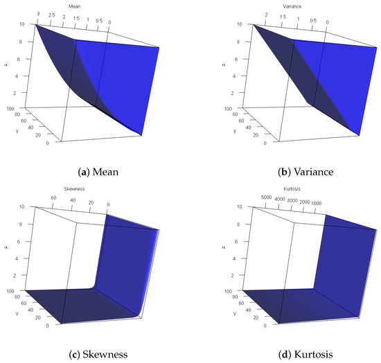
Figure 2. Three-dimensional plots for the DMB characteristics.

3.2. Order Statistics

Taking $(Y_1,Y_2,\dots ,Y_n)$ as a random sample from the DGM model and assuming that $(Y_{1:n},Y_{2:n},\dots ,Y_{n:n})$ represent their related order statistics, the order statistics have a CDF at y, whereby

$$F_{i:n}(y;\alpha )=\sum _{m=i}^n\left({\displaystyle \genfrac{}{}{0pt}{}{n}{m}}\right){\left[F(y_i;\alpha )\right]}^m{[1-F(y_i;\alpha )]}^{n-m}.$$

(15)

The CDF can be represented as a series using the negative binomial theorem, which can be expressed as

$$F_{i:n}(y;\alpha )=\sum _{i=1}^n\sum _{j=1}^{n-m}\left({\displaystyle \genfrac{}{}{0pt}{}{n}{m}}\right)\left({\displaystyle \genfrac{}{}{0pt}{}{n-m}{j}}\right){(-1)}^j{\left[F(y_i;\alpha )\right]}^{m+j}.$$

(16)

Consequently,

$$F_{i:n}(y;\alpha )=\sum _{i=1}^n\sum _{j=1}^{n-m}\left({\displaystyle \genfrac{}{}{0pt}{}{n}{m}}\right)\left({\displaystyle \genfrac{}{}{0pt}{}{n-m}{j}}\right){(-1)}^j{[1-\Omega (\alpha ;y_i+1)]}^{m+j}.$$

(17)

The PMF for the i-th order statistic in the DMB model is as follows:

$$f_{i:n}(y;\alpha )=\sum _{i=1}^n\sum _{j=1}^{n-m}\left({\displaystyle \genfrac{}{}{0pt}{}{n}{m}}\right)\left({\displaystyle \genfrac{}{}{0pt}{}{n-m}{j}}\right){(-1)}^j{[\Omega (\alpha ;y_i)-\Omega (\alpha ;y_i+1)]}^{m+j}.$$

(18)

4. DMB Parameter Estimation

In this section, we estimate the DMB parameter $\alpha$ by applying the maximum likelihood and Bayesian estimation methodologies.

4.1. Maximum Likelihood Estimator

This part develops the MLE $\widehat{\alpha }$ of $\alpha$ under a T2C strategy. Let $\mathbf{y}=y_1,y_2,\dots ,y_r$ denote a T2C sample from the DMB distribution. Using (4) and (5), the likelihood function (symbolized by $\mathcal{L}(·)$) and the corresponding log-likelihood function (symbolized by ${\mathcal{L}}^{★}(·)$) are given, by setting $I_{j,i}\left(\alpha \right)\equiv I_j(y_i;\alpha ),j=1,2$, respectively, by

$$\mathcal{L}(\alpha \mid \mathbf{y})\propto \prod _{i=1}^r\left\{c\left(\alpha \right)[I_{1,i}\left(\alpha \right)-I_{2,i}\left(\alpha \right)]\right\}{\left[c\left(\alpha \right)I_{1,r}\left(\alpha \right)\right]}^{n-r},$$

(19)

and

$${\mathcal{L}}^{★}(\alpha \mid \mathbf{y})=\sum _{i=1}^{r}ln\left(c\left(\alpha \right)[I_{1,i}\left(\alpha \right)-I_{2,i}\left(\alpha \right)]\right)+(n-r)ln\left(c\left(\alpha \right)I_{1,r}\left(\alpha \right)\right),$$

(20)

where $c\left(\alpha \right)={\displaystyle \frac{4}{{\alpha }^3\sqrt{\pi }}},$ $I_{1,i}\left(\alpha \right)={\int }_{x_i}^{\infty }{y}^2{e}^{-y^2/\alpha }dy$, and $I_{2,i}\left(\alpha \right)={\int }_{x_i}^{\infty }{(y+1)}^2{e}^{-{(y+1)}^2/\alpha }dy$.

Differentiating (20), the normal equation of $\alpha$ (which must be equated to zero to get its corresponding MLE $\widehat{\alpha }$) can be written as follows:

$${\left.{\displaystyle \frac{d{\mathcal{L}}^{★}}{d\alpha }}=-{\displaystyle \frac{3n}{\alpha }}+{\displaystyle \frac{1}{{\alpha }^2}}\left[\sum _{i=1}^r{\displaystyle \frac{I_{1,i}^{\circ }\left(\alpha \right)-I_{2,i}^{\circ }\left(\alpha \right)}{I_{1,i}\left(\alpha \right)-I_{2,i}\left(\alpha \right)}}+(n-r){\displaystyle \frac{I_{1,r}^{\circ }\left(\alpha \right)}{I_{1,r}\left(\alpha \right)}}\right]\right|}_{\alpha =\widehat{\alpha }}=0,$$

(21)

where $I_{1,i}^{\circ }\left(\alpha \right)={\int }_{x_i}^{\infty }{y}^4{e}^{-y^2/\alpha }dy$, and $I_{2,i}^{\circ }\left(\alpha \right)={\int }_{x_i}^{\infty }{(y+1)}^4{e}^{-{(y+1)}^2/\alpha }dy.$

Remark 2.

The closed-form expressions for the integrals $I_i(·)$ and $I_i^{\circ }(·)$ for $i=1,2$ cannot be obtained analytically in terms of incomplete gamma functions. Therefore, it is often preferable to compute the MLE $\widehat{\alpha }$ using the Newton–Raphson ($\mathsf{NR}$) iterative method. For this purpose, the $\mathsf{NR}$ method is implemented via the maxNR command, which is available in the maxLik package (by Henningsen and Toomet [20]).

We now investigate the existence and uniqueness of the MLE $\widehat{\alpha }$. Owing to the complicated structure of the gradient equation in (21), it is analytically intractable to establish these properties in closed form. Consequently, a numerical assessment is conducted by simulating a T2C sample from the DMB distribution for $\alpha \in \{1.5,2.5\}$ with $(n,r)\in \{40,20\}$. The resulting MLEs of $\alpha$ are $1.9292$ and $3.7003$, respectively. Figure 3 displays the log-likelihood function in (20) and the corresponding score function in (21) as functions of $\alpha$ over a specified range. In each case, the vertical line denoting the MLE intersects the log-likelihood curve at its maximum (red line) and the score function (blue line) at zero. These numerical findings verify that the MLE of $\alpha$ exists and is unique for the considered scenarios.

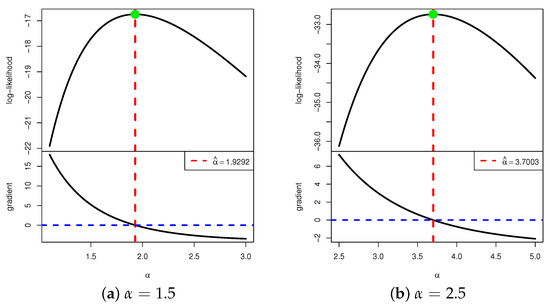
Figure 3. The log-likelihood curve versus its gradient function curve for DMB $\left(\alpha \right)$.

4.2. Bayesian Estimator

This section discusses Bayesian estimation, which is used to estimate the unknown parameters of the DMB model. This method interprets the parameters as random variables that follow a specific model, known as the prior distribution. Because prior knowledge is frequently unavailable, it becomes vital to select an appropriate prior. A joint conjugate prior distribution is chosen for parameters $\alpha$, with each parameter assumed to have a gamma distribution. Hence, $\alpha \sim Gamma(a,b)$ represent non-negative hyper-parameters of the given distributions. The prior distribution for $\alpha$, say $\varrho \left(\alpha \right)$, is defined as follows:

$$\varrho \left(\alpha \right)={\displaystyle \frac{b^a}{\Gamma \left(a_1\right)}}{\alpha }^{a-1}{e}^{-b\alpha },a,b,\alpha >0,$$

(22)

where ($a,b$) represents non-negative hyper-parameters of the DMB distribution parameter.

Given the objective T2C data $\mathbf{y}$, the posterior PDF of $\alpha$, say $\rho (·)$, can be represented as

$$\rho \left(\alpha \right|\mathbf{y})={\Im }^{-1}\varrho \left(\alpha \right)\mathcal{L}(\alpha \mid \mathbf{y}),$$

(23)

where $\Im (={\int }_0^{\infty }\varrho \left(\alpha \right)\mathcal{L}(\alpha \mid \mathbf{y})d\alpha )$ is the normalized term that does not depend on $\alpha$.

From (22) and (19), we can redefine (23) as follows:

$$\rho \left(\alpha \right|\mathbf{y})={\Im }^{-1}{\alpha }^{a-1}{e}^{-b\alpha }\prod _{i=1}^r\left\{c\left(\alpha \right)[I_{1,i}\left(\alpha \right)-I_{2,i}\left(\alpha \right)]\right\}{\left[c\left(\alpha \right)I_{1,r}\left(\alpha \right)\right]}^{n-r}.$$

(24)

The squared-error loss (SEL) function has been used to examine the DMB model’s parameter estimate. Afterward, to assess the effectiveness of the estimation approaches and investigate how the parameter values affect them, a simulated analysis is conducted to evaluate the estimators’ effectiveness using several measure.

The Bayesian estimate of a parameter $\alpha$, say $\tilde{\alpha }$, is defined under the SEL as the expected value for the posterior distribution, such as

$$\begin{array}{cc}\hfill \tilde{\alpha }& =\mathbb{E}\left[\alpha \right|\mathbf{y}]\hfill \\ \hfill & ={\Im }^{-1}{\int }_0^{\infty }{\alpha }^a{e}^{-b\alpha }\prod _{i=1}^r\left\{c\left(\alpha \right)[I_{1,i}\left(\alpha \right)-I_{2,i}\left(\alpha \right)]\right\}{\left[c\left(\alpha \right)I_{1,r}\left(\alpha \right)\right]}^{n-r}\mathrm{d}\alpha .\hfill \end{array}$$

(25)

It is important to use numerical methods to compute the integration described in Equation (25). The Metropolis–Hastings (M-H) sampler, a fundamental concept in the MCMC family of Bayesian computation algorithms, was developed to solve this problem. A suitable R code was produced based on Algorithm 1 to implement this method. In doing so, we used the MCMC iterative approach beyond just providing the conditional posterior PDF of $\alpha$ as

$$\begin{array}{c}\hfill \mathcal{O}\left(\alpha \right|\mathbf{y})\propto {\alpha }^{a-1}{e}^{-b\alpha }\prod _{i=1}^r\left\{c\left(\alpha \right)[I_{1,i}\left(\alpha \right)-I_{2,i}\left(\alpha \right)]\right\}{\left[c\left(\alpha \right)I_{1,r}\left(\alpha \right)\right]}^{n-r}.\end{array}$$

(26)

Algorithm 1 The M-H Algorithm for Sampling $\alpha$

1:   Input: Initial estimate $\widehat{\alpha }$, estimated variance $\widehat{Var}\left(\widehat{\alpha }\right)$, total iterations $\mathbb{M}$, burn-in ${\mathbb{M}}^{\circ }$, confidence level $(1-\epsilon )$ 2:   Output: Posterior mean $\tilde{\alpha }$ 3:   Set ${\alpha }^{\left(0\right)}\leftarrow \widehat{\alpha }$ 4:   Set $j\leftarrow 1$ 5:   while$j\le \mathbb{M}$do 6:         Generate ${\alpha }^{★}\sim N({\alpha }^{(j-1)},\widehat{Var}\left(\widehat{\alpha }\right)$ 7:         Compute acceptance ratio: $$M\leftarrow min\left(1,{\displaystyle \frac{\mathcal{O}({\alpha }^{★}\mid \mathbf{y})}{\mathcal{O}({\alpha }^{(j-1)}\mid \mathbf{y})}}\right)$$ 8:         Generate $u\sim U(0,1)$ 9:         if $u\le M$ then 10:           Set ${\alpha }^{\left(j\right)}\leftarrow {\alpha }^{★}$ 11:       else 12:           Set ${\alpha }^{\left(j\right)}\leftarrow {\alpha }^{(j-1)}$ 13:       end if 14:       Increment $j\leftarrow j+1$ 15: end while 16: Discard the first ${\mathbb{M}}^{\circ }$ samples as burn-in 17: Define ${\mathbb{M}}^{•}=\mathbb{M}-{\mathbb{M}}^{\circ }$ 18: Compute: $$\tilde{\alpha }={\displaystyle \frac{1}{{\mathbb{M}}^{•}}}\sum _{j={\mathbb{M}}^{\circ }+1}^{\mathbb{M}}{\alpha }^{\left(j\right)}$$

5. Interval Estimation

This section presents six different interval estimation methods for the DMB($\alpha$) parameter, including two bootstrapping methods, two asymptotic confidence interval methods, and two credible interval methods. These estimators are derived under different inferential paradigms, frequentist, bootstrap-based, and Bayesian, each offering distinct theoretical foundations and practical characteristics. The subsequent subsections describe the formulation, computational procedures, and interpretation of each method in detail.

5.1. Asymptotic Intervals

To construct the asymptotic confidence interval (ACI) for the DMB parameter $\alpha$, the variance of $\widehat{\alpha }$ is obtained from the Fisher information matrix (FIM), denoted by $\mathcal{I}\left(\alpha \right)$, which is derived as follows:

$$\mathcal{I}\left(\alpha \right)=-\mathbb{E}\left[{\displaystyle \frac{{\mathrm{d}}^2{\mathcal{L}}^{★}}{\mathrm{d}{\alpha }^2}}\right],$$

(27)

where the expectation operator $\mathbb{E}$ is taken under the existing distribution of $\widehat{\alpha }$. However, for censored (or complex) data models, the observed information is often preferred due to its computational tractability. Thus, the expectation operator $\mathbb{E}$ is dropped in practice; see Lawless [21].

The inverse of the FIM yields the variance, which is then used to construct the ACI for the DMB parameter $\alpha$. In practice, one may employ the observed FIM—the negative of the Hessian matrix of ${\mathcal{L}}^{★}$ evaluated at the MLE $\widehat{\alpha }$—to approximate its variance, i.e., $\widehat{Var}\left(\widehat{\alpha }\right)\approx {\mathcal{I}}_{\mathrm{obs}}^{-1}\left(\widehat{\alpha }\right){|}_{(\alpha =\widehat{\alpha })}$. As a result, to get the quantity of $\widehat{Var}\left(\widehat{\alpha }\right)$, where $I_{1,i}^{\circ }\equiv I_{1,i}^{\circ }\left(\alpha \right)$, we use

$$\begin{array}{cc}\hfill {\displaystyle \frac{{\mathrm{d}}^2{\mathcal{L}}^{★}}{\mathrm{d}{\alpha }^2}}& =-{\displaystyle \frac{3n}{{\alpha }^2}}+{\displaystyle \frac{2}{{\alpha }^3}}\left[\sum _{i=1}^r{\displaystyle \frac{I_{1,i}^{\circ }-I_{2,i}^{\circ }}{I_{1,i}-I_{2,i}}}+(n-r){\displaystyle \frac{I_{1,r}^{\circ }}{I_{1,r}}}\right]\hfill \\ \hfill & -{\displaystyle \frac{1}{{\alpha }^4}}\left[\sum _{i=1}^r{\displaystyle \frac{(K_{1,i}-K_{2,i})(I_{1,i}-I_{2,i})-{(I_{1,i}^{\circ }-I_{2,i}^{\circ })}^2}{{(I_{1,i}-I_{2,i})}^2}}+(n-r){\displaystyle \frac{K_{1,r}{I}_{1,r}-{\left(I_{1,r}^{\circ }\right)}^2}{I_{1,r}^2}}\right],\hfill \end{array}$$

(28)

where $K_{1,i}\equiv K_{1,i}\left(\alpha \right)={\int }_{x_i}^{\infty }{y}^6{e}^{-y^2/\alpha }dy$, and $K_{2,i}\equiv K_{2,i}\left(\alpha \right)={\int }_{x_i}^{\infty }{(y+1)}^6{e}^{-{(y+1)}^2/\alpha }dy$.

Now, from (28), we can utilize the asymptotic normality approximation (NA) of the MLE $\widehat{\alpha }$, which is normally distributed with mean $\alpha$ and variance $\widehat{Var}\left(\widehat{\alpha }\right)$. As a consequence, at a significance level $\epsilon \%$, the $(1-\epsilon )100\%$ ACI using NA-based (ACI[NA]) of $\alpha$ is given by

$$\left(\widehat{\alpha }\mp z_{{\displaystyle \frac{\epsilon }{2}}}\sqrt{\widehat{Var}\left(\widehat{\alpha }\right)}\right),$$

where $z_{\epsilon /2}$ is the upper $0.5\epsilon$ percentile of the standard normal distribution.

A well-recognized limitation of the ACI[NA] is its potential to produce negative lower bound of $\widehat{\alpha }$ that is, by definition, restricted to positive values. In practice, such negative bounds are often replaced with zero; however, this constitutes a heuristic adjustment rather than a principled statistical remedy. To overcome this limitation and enhance the reliability of interval estimation, Meeker and Escobar [22] proposed the use of the $(1-\epsilon )100\%$ ACI based on the log-transformed-NL (ACI[NL]), which is given by

$$\widehat{\alpha }exp\left(\mp z_{{\displaystyle \frac{\epsilon }{2}}}{\widehat{\alpha }}^{-1}\sqrt{\widehat{Var}\left(\widehat{\alpha }\right)}\right).$$

5.2. Bootstrap Intervals

For small complete sample sizes (n), the performance of ACI[NA] (or ACI[NL]) approach is often unsatisfactory, as their validity relies on large-sample properties implied by the law of large numbers. To improve interval estimation under such conditions, two resampling-based procedures are employed: the bootstrap-p and bootstrap-t algorithms. These methods are applied to estimate the interval bounds of the DMB($\alpha$) parameter. The computation of the $100(1-\epsilon )\%$ bootstrap-p (or bootstrap-t) intervals for these quantities begins by generating a bootstrap sample, as described in Algorithm 2. For additional details on creating bootstrap estimates in the R environment, see Chernick and LaBudde [23].

5.3. Credible Intervals

In the Bayesian framework, a BCI specifies a range of parameter values that, given the observed data and prior information, contain the true parameter with a stated posterior probability. Unlike the frequentist confidence interval, which is defined through the long-run behavior of repeated sampling, the BCI has a direct probabilistic interpretation. The BCI bounds are commonly reported either as HPD interval bounds, which include the most probable parameter values, or as equal-tailed intervals, which assign identical posterior probabilities to each tail of the distribution. In this part, via the MCMC sampling procedure described in Algorithm 1, both BCI and HPD methods are constructed; see Algorithm 3.

Algorithm 2 Bootstrapping Confidence Intervals for $\alpha$

1:   Compute the MLE $\widehat{\alpha }$ from the original sample. 2:   for$j=1$ to $\mathbb{B}$ do 3:         Generate a bootstrap sample $\{Y_1^{*},Y_2^{*},\dots ,Y_r^{*}\}$ from $\mathrm{DMB}\left(\widehat{\alpha }\right)$. 4:         Compute ${\widehat{\alpha }}_j^{*}$ (MLE from the bootstrap sample). 5:   end for 6:   Sort the bootstrap estimates in ascending order: ${\widehat{\alpha }}_{\left(1\right)}^{*}<\cdots <{\widehat{\alpha }}_{\left(\mathbb{B}\right)}^{*}$. 7:   Bootstrap-p (Percentile) Interval (BP): 8:   $\mathrm{Lower}\leftarrow {\widehat{\alpha }}_{\left[\mathbb{B}\left({\displaystyle \frac{\epsilon }{2}}\right)\right]}^{*}$ 9:   $\mathrm{Upper}\leftarrow {\widehat{\alpha }}_{\left[\mathbb{B}(1-{\displaystyle \frac{\epsilon }{2}})\right]}^{*}$ 10: Boot-p$\mathrm{Interval}\leftarrow (\mathrm{Lower},\mathrm{Upper})$ 11: Bootstrap-t Interval (BT): 12: for$j=1$ to $\mathbb{B}$ do 13:       $T_j^{\alpha }\leftarrow {\displaystyle \frac{{\widehat{\alpha }}_j^{*}-\widehat{\alpha }}{\sqrt{\widehat{Var}\left(\widehat{\alpha }\right)}}}$ 14: end for 15: Sort T-statistics: $T_{\left(1\right)}^{\alpha }<\cdots <T_{\left(\mathbb{B}\right)}^{\alpha }$ 16: $\mathrm{Lower}\leftarrow \widehat{\alpha }-T_{\left[\mathbb{B}(1-{\displaystyle \frac{\epsilon }{2}})\right]}^{\alpha }\times \sqrt{\widehat{Var}\left(\widehat{\alpha }\right)}$ 17: $\mathrm{Upper}\leftarrow \widehat{\alpha }-T_{\left[\mathbb{B}\left({\displaystyle \frac{\epsilon }{2}}\right)\right]}^{\alpha }\times \sqrt{\widehat{Var}\left(\widehat{\alpha }\right)}$ 18: Boot-t$\mathrm{Interval}\leftarrow (\mathrm{Lower},\mathrm{Upper})$

Algorithm 3 The BCI and HPD Interval Estimates for $\alpha$

1: Input: Collect MCMC estimates ${\alpha }^{\left(j\right)}$ for $j={\mathbb{M}}^{\circ }+1,\dots ,\mathbb{M}$ 2: Output: The $(1-\epsilon )100\%$ BCI and HPD estimates of $\alpha$ 3: Set ${\alpha }^{\left(j\right)}$ for $j={\mathbb{M}}^{\circ }+1,\dots ,\mathbb{M}$ in ascending order as: $${\alpha }_{({\mathbb{M}}^{\circ }+1)},{\alpha }_{({\mathbb{M}}^{\circ }+2)},\dots {\alpha }_{\left(\mathbb{M}\right)},$$ 4: Compute the $(1-\epsilon )100\%$ BCI of $\alpha$ as: $$\left({\alpha }_{\left({\displaystyle \frac{\epsilon }{2}}{\mathbb{M}}^{•}\right)},{\alpha }_{\left(\left(1-{\displaystyle \frac{\epsilon }{2}}\right){\mathbb{M}}^{•}\right)}\right)$$ 5: Compute the $(1-\epsilon )100\%$ HPD interval of $\alpha$ as: $$\left({\alpha }_{\left(j^{⊚}\right)},{\alpha }_{(j^{⊚}+(1-\epsilon ){\mathbb{M}}^{•})}\right)$$ where $j^{⊚}$ is the index that minimizes: $${\alpha }_{\left(j+(1-\epsilon ){\mathbb{M}}^{•}\right)}-{\alpha }_{\left(j\right)}\mathrm{for}j=1,\dots ,\epsilon {\mathbb{M}}^{•}$$

6. Simulation Comparisons

In this part, we conduct an extensive Monte Carlo simulation analysis to evaluate the associated behavior of the proposed estimators for the parameters of DMB($\alpha$) distribution. From this investigation, we conclude a discussion that provides a comprehensive examination of the experimental results obtained.

6.1. Simulation Setups

To generate T2C samples from the DMB($\alpha$) distribution and to establish the simulation setup for evaluating the proposed estimation procedures, we performed the following structured steps:

Step 1:

Specify the true parameter configurations of the DMB ($\alpha$) distribution:

• Pop-1: DMB (0.8);
• Pop-2: DMB (1.5).

Step 2:

Select the sample sizes: $n\in \{20,40,80,100,150,200,250,300\}$.

Step 3:

Generate n independent pseudo-random values from the uniform $U(0,1)$ distribution, say $u_i$ for $i=1,2,\dots ,n$.

Step 4:

Generate complete samples (with size n) from the DMB($\alpha$) distribution as

$$x_i=F^{-1}(u_i;\alpha ),i=1,2,\dots ,n.$$

Step 5:

Sort $x_i$ for $i=1,2,\dots ,n$ in ascending order.

Step 6:

Specify the failure percentage (FP%) as

$$\mathrm{FP}=\left({\displaystyle \frac{m}{n}}\right)\times 100\%\mathrm{where}\mathrm{FP}\%\in \{25,50,75,100\%\}.$$

Step 7:

Replicate Steps 2–6 5000 times.

Step 8:

Specify the hyperparameters $(a,b)$:

• For Prior 1: $(3.2,5)$ and (6, 5) for Pop-$i,i=1,2$, respectively;
• For Prior 2: $(6.4,9)$ and (12, 9) for Pop-$i,i=1,2$, respectively.

Step 9:

Set $\mathbb{M}=10,000$ and ${\mathbb{M}}^{\circ }$ = 2000 for Bayes’ computations.

Step 10:

Set $\mathbb{B}=10,000$ for bootstrapping computations.

Step 11:

For point estimates (including likelihood and Bayes), compute the following evaluation metrics:

• Average Point Estimate (APE):

  $$\mathrm{APE}\left(\check{\alpha }\right)={\displaystyle \frac{1}{5000}}\sum _{i=1}^{5000}{\check{\alpha }}^{\left[i\right]};$$
• Root Mean Squared Error (RMSE):

  $$\mathrm{RMSE}\left(\check{\alpha }\right)=\sqrt{{\displaystyle \frac{1}{5000}}\sum _{i=1}^{5000}{\left({\check{\alpha }}^{\left[i\right]}-\alpha \right)}^2};$$
• Mean Relative Absolute Bias (MRAB):

  $$\mathrm{MRAB}\left(\check{\alpha }\right)={\displaystyle \frac{1}{5000}}\sum _{i=1}^{5000}{\alpha }^{-1}\left|{\check{\alpha }}^{\left[i\right]}-\alpha \right|,$$

  where ${\check{\alpha }}^{\left[i\right]}$ denotes the ith point estimate of $\alpha$.

Step 12:

For point estimates (including BP, BT, ACI[NA], ACI[NL], BCI, and HPD), compute the following evaluation metrics:

• Average Interval Length (AIL):

  $${\mathrm{AIL}}_{95\%}\left(\alpha \right)={\displaystyle \frac{1}{5000}}\sum _{i=1}^{5000}\left({\mathcal{U}}_{{\check{\alpha }}^{\left[i\right]}}-{\mathcal{L}}_{{\check{\alpha }}^{\left[i\right]}}\right);$$
• Coverage Probability (CP) at 95% level:

  $${\mathrm{CP}}_{95\%}\left(\alpha \right)={\displaystyle \frac{1}{5000}}\sum _{i=1}^{5000}{\mathbb{I}}_{[{\mathcal{L}}_{{\check{\alpha }}^{\left[i\right]}},{\mathcal{U}}_{{\check{\alpha }}^{\left[i\right]}}]}\left(\alpha \right),$$

  where $({\mathcal{L}}_{{\check{\alpha }}^{\left[i\right]}}$ and ${\mathcal{U}}_{{\check{\alpha }}^{\left[i\right]}})$ denote the lower and upper interval bounds, respectively.

6.2. Simulation Outcomes and Discussion

Table 2, Table 3, Table 4 and Table 5 summarize the simulation findings for each group of model parameters. Specifically, in Table 2, Table 3, Table 4 and Table 5, the APEs, RMSEs, and MRABs are reported in the first, second, and third columns, respectively. In Table 4 and Table 5, the AILs and CPs are reported in the first and second columns, respectively. Several assessments and recommendations are drawn from Table 2, Table 3, Table 4 and Table 5 based on the lowest RMSE, MRAB, and AIL values, as well as the highest CP values, as follows:

Table 2. The point estimation results of $\alpha$ from Pop-1.

FP%	n	MLE			Bayes [Prior 1]			Bayes [Prior 2]
25%	20	1.350	2.237	2.772	0.927	1.486	1.814	0.903	0.800	0.957
	40	1.346	2.215	2.763	1.093	1.349	1.657	1.043	0.695	0.830
	80	1.346	2.086	2.491	1.226	1.191	1.441	1.056	0.625	0.739
	100	1.346	1.999	2.487	1.493	0.910	1.112	1.014	0.459	0.542
	150	1.353	1.992	2.381	1.442	0.788	0.967	1.072	0.418	0.494
	200	1.346	1.901	2.364	1.689	0.679	0.811	1.128	0.349	0.410
	250	1.350	1.891	2.282	1.573	0.464	0.532	1.199	0.257	0.304
	300	1.346	1.745	1.954	1.658	0.310	0.367	1.222	0.188	0.268
50%	20	1.313	2.230	2.768	0.963	1.442	1.764	0.874	0.797	0.951
	40	1.284	2.212	2.762	1.070	1.243	1.528	1.037	0.692	0.828
	80	1.246	2.016	2.488	1.194	1.182	1.427	1.046	0.616	0.730
	100	1.220	1.996	2.486	1.449	0.877	1.072	1.001	0.451	0.541
	150	1.182	1.989	2.376	1.970	0.747	0.919	1.391	0.403	0.474
	200	1.159	1.899	2.364	2.251	0.678	0.803	1.464	0.303	0.341
	250	1.142	1.891	2.209	1.468	0.429	0.493	1.165	0.253	0.296
	300	1.118	1.690	1.899	1.535	0.285	0.344	1.195	0.188	0.260
75%	20	1.500	2.226	2.766	1.153	1.413	1.733	0.955	0.732	0.881
	40	1.506	2.212	2.758	1.382	1.214	1.489	1.175	0.688	0.822
	80	1.509	2.005	2.487	1.598	1.122	1.345	1.232	0.466	0.559
	100	1.507	1.993	2.486	1.876	0.849	1.016	1.235	0.448	0.528
	150	1.503	1.912	2.374	1.942	0.739	0.867	1.384	0.398	0.468
	200	1.506	1.891	2.364	2.211	0.620	0.749	1.458	0.268	0.321
	250	1.505	1.891	2.116	2.022	0.368	0.441	1.504	0.233	0.287
	300	1.505	1.646	1.855	2.147	0.175	0.320	1.561	0.108	0.253
100%	20	1.395	2.221	2.765	1.149	1.373	1.684	0.954	0.728	0.876
	40	1.395	2.211	2.749	1.399	1.210	1.462	1.179	0.635	0.753
	80	1.396	2.000	2.487	1.612	1.086	1.304	1.247	0.461	0.544
	100	1.395	1.992	2.484	1.843	0.836	0.997	1.234	0.420	0.499
	150	1.394	1.905	2.364	1.953	0.688	0.835	1.402	0.384	0.457
	200	1.395	1.891	2.364	2.186	0.603	0.728	1.462	0.260	0.307
	250	1.395	1.837	2.049	1.992	0.364	0.437	1.500	0.219	0.275
	300	1.394	1.585	1.796	2.125	0.163	0.312	1.566	0.107	0.246

Table 3. The point estimation results of $\alpha$ from Pop-2.

FP%	n	MLE			Bayes [Prior 1]			Bayes [Prior 2]
25%	20	2.149	1.803	2.091	1.488	1.302	0.843	1.520	0.604	0.378
	40	2.318	1.573	2.089	1.475	1.163	0.749	1.656	0.488	0.304
	80	1.968	1.568	1.866	1.530	1.041	0.657	1.614	0.416	0.258
	100	2.009	1.282	1.672	2.376	0.926	0.584	1.753	0.344	0.204
	150	2.014	1.256	1.669	2.236	0.864	0.538	1.812	0.275	0.172
	200	2.318	1.244	1.557	2.170	0.500	0.303	1.886	0.264	0.161
	250	1.933	1.171	1.553	1.770	0.276	0.170	1.584	0.167	0.104
	300	2.002	1.166	1.272	1.861	0.155	0.095	1.583	0.098	0.056
50%	20	1.890	1.637	2.091	1.644	1.245	0.802	1.559	0.539	0.340
	40	2.319	1.571	2.089	1.755	1.124	0.726	1.719	0.453	0.285
	80	1.917	1.567	1.686	1.979	1.016	0.641	1.759	0.398	0.247
	100	2.005	1.264	1.670	2.341	0.926	0.577	1.742	0.331	0.204
	150	1.831	1.255	1.669	2.332	0.841	0.526	1.806	0.272	0.169
	200	2.317	1.243	1.557	2.065	0.374	0.241	1.870	0.260	0.159
	250	1.918	1.171	1.553	2.246	0.264	0.163	1.927	0.121	0.076
	300	2.004	1.166	1.242	2.124	0.120	0.062	2.003	0.095	0.048
75%	20	1.704	1.594	2.091	1.643	1.221	0.790	1.557	0.537	0.336
	40	2.316	1.568	2.088	1.745	1.094	0.707	1.713	0.436	0.270
	80	1.914	1.484	1.679	1.955	0.992	0.637	1.752	0.388	0.240
	100	2.002	1.261	1.670	2.307	0.902	0.561	1.738	0.331	0.201
	150	1.681	1.255	1.624	2.288	0.625	0.386	1.794	0.269	0.168
	200	2.317	1.212	1.553	2.259	0.354	0.221	1.861	0.236	0.146
	250	1.915	1.166	1.520	2.040	0.240	0.151	1.906	0.112	0.057
	300	2.002	1.098	1.139	2.156	0.092	0.046	1.979	0.077	0.043
100%	20	1.604	1.578	2.090	1.727	1.188	0.766	1.576	0.514	0.320
	40	2.317	1.568	2.088	1.832	1.087	0.707	1.749	0.431	0.264
	80	1.915	1.410	1.674	2.078	0.940	0.601	1.802	0.351	0.208
	100	2.003	1.259	1.670	2.455	0.888	0.555	1.806	0.318	0.196
	150	1.581	1.253	1.577	2.249	0.525	0.319	1.897	0.265	0.166
	200	2.316	1.195	1.553	2.176	0.280	0.180	1.956	0.229	0.142
	250	1.915	1.166	1.441	2.256	0.157	0.096	2.009	0.104	0.057
	300	2.002	1.063	1.108	2.169	0.062	0.031	2.066	0.055	0.028

Table 4. The interval estimation results of $\alpha$ from Pop-1.

FP%	n	BP		BT		ACI [NA]		ACI [NL]		BCI [Prior 1]		BCI [Prior 2]		HPD [Prior 1]		HPD [Prior 2]
25%	20	2.604	0.881	2.604	0.881	2.737	0.875	2.872	0.869	1.142	0.945	0.786	0.948	1.077	0.961	0.763	0.962
	40	2.036	0.906	2.036	0.906	2.118	0.902	2.169	0.900	1.009	0.951	0.662	0.952	0.988	0.966	0.643	0.967
	80	1.692	0.921	1.666	0.922	1.836	0.915	1.836	0.915	0.885	0.957	0.640	0.958	0.846	0.967	0.626	0.968
	100	0.797	0.960	0.779	0.961	1.264	0.940	1.277	0.939	0.741	0.963	0.468	0.963	0.741	0.975	0.464	0.975
	150	0.697	0.965	0.672	0.966	1.060	0.949	1.067	0.948	0.603	0.969	0.432	0.972	0.529	0.977	0.423	0.977
	200	0.613	0.968	0.602	0.969	0.926	0.955	0.929	0.955	0.495	0.974	0.389	0.975	0.472	0.978	0.382	0.979
	250	0.457	0.975	0.441	0.976	0.749	0.963	0.752	0.962	0.430	0.977	0.316	0.977	0.422	0.982	0.309	0.982
	300	0.393	0.978	0.373	0.979	0.654	0.967	0.655	0.967	0.368	0.979	0.263	0.980	0.362	0.984	0.259	0.984
50%	20	2.360	0.892	2.357	0.892	2.657	0.878	2.772	0.873	1.063	0.949	0.775	0.949	1.048	0.961	0.752	0.962
	40	1.900	0.912	1.862	0.913	1.927	0.911	1.927	0.911	0.993	0.952	0.661	0.954	0.946	0.966	0.643	0.967
	80	1.246	0.941	1.246	0.941	1.498	0.930	1.516	0.929	0.841	0.958	0.628	0.959	0.824	0.968	0.615	0.968
	100	0.774	0.961	0.759	0.962	1.178	0.944	1.187	0.943	0.690	0.965	0.455	0.965	0.690	0.975	0.445	0.976
	150	0.693	0.965	0.658	0.967	1.060	0.949	1.066	0.949	0.588	0.970	0.417	0.974	0.495	0.977	0.406	0.978
	200	0.607	0.969	0.589	0.970	0.879	0.957	0.884	0.957	0.482	0.974	0.381	0.977	0.430	0.979	0.371	0.979
	250	0.430	0.977	0.414	0.977	0.717	0.964	0.719	0.964	0.408	0.978	0.303	0.978	0.393	0.982	0.296	0.982
	300	0.383	0.979	0.360	0.980	0.599	0.969	0.600	0.969	0.358	0.980	0.251	0.980	0.351	0.984	0.249	0.985
75%	20	2.139	0.901	2.139	0.901	2.634	0.879	2.740	0.875	1.052	0.949	0.672	0.952	0.994	0.966	0.654	0.967
	40	1.877	0.913	1.838	0.915	1.913	0.911	1.914	0.911	0.992	0.952	0.654	0.955	0.928	0.967	0.641	0.967
	80	1.065	0.949	1.062	0.949	1.375	0.935	1.390	0.934	0.832	0.959	0.502	0.960	0.806	0.973	0.491	0.974
	100	0.746	0.963	0.738	0.963	1.134	0.946	1.141	0.945	0.651	0.967	0.454	0.967	0.650	0.976	0.443	0.976
	150	0.622	0.968	0.613	0.969	0.962	0.953	0.967	0.953	0.529	0.972	0.401	0.974	0.487	0.978	0.393	0.978
	200	0.573	0.970	0.556	0.971	0.801	0.960	0.804	0.960	0.479	0.974	0.362	0.977	0.429	0.980	0.357	0.980
	250	0.419	0.977	0.399	0.978	0.670	0.966	0.671	0.966	0.395	0.978	0.281	0.978	0.387	0.983	0.276	0.983
	300	0.369	0.979	0.352	0.980	0.592	0.969	0.594	0.969	0.350	0.980	0.239	0.980	0.345	0.985	0.237	0.985
100%	20	2.083	0.904	2.083	0.904	2.526	0.884	2.601	0.881	1.040	0.950	0.665	0.952	0.991	0.966	0.652	0.967
	40	1.819	0.915	1.793	0.917	1.877	0.913	1.878	0.913	0.973	0.953	0.641	0.955	0.926	0.967	0.627	0.968
	80	0.970	0.953	0.969	0.953	1.269	0.940	1.279	0.939	0.802	0.960	0.475	0.961	0.783	0.975	0.471	0.975
	100	0.717	0.964	0.703	0.965	1.108	0.947	1.118	0.946	0.634	0.968	0.450	0.969	0.603	0.976	0.439	0.976
	150	0.618	0.968	0.605	0.969	0.947	0.954	0.952	0.954	0.516	0.973	0.393	0.974	0.479	0.978	0.385	0.979
	200	0.525	0.972	0.518	0.973	0.773	0.961	0.775	0.961	0.467	0.975	0.361	0.977	0.424	0.980	0.356	0.980
	250	0.419	0.977	0.379	0.979	0.661	0.966	0.663	0.966	0.368	0.979	0.263	0.979	0.365	0.984	0.260	0.984
	300	0.342	0.980	0.198	0.987	0.546	0.971	0.547	0.971	0.197	0.987	0.231	0.987	0.193	0.985	0.224	0.986

Table 5. The interval estimation results of $\alpha$ from Pop-2.

FP%	n	BP		BT		ACI [NA]		ACI [NL]		BCI [Prior 1]		BCI [Prior 2]		HPD [Prior 1]		HPD [Prior 2]
25%	20	4.876	0.848	4.764	0.851	5.183	0.841	5.325	0.837	1.135	0.943	0.686	0.954	1.120	0.943	0.675	0.955
	40	3.293	0.888	3.227	0.890	4.440	0.859	4.441	0.859	1.070	0.945	0.559	0.958	1.038	0.945	0.549	0.958
	80	2.162	0.917	2.159	0.917	2.282	0.914	2.305	0.913	1.011	0.946	0.497	0.959	0.979	0.947	0.486	0.959
	100	1.382	0.937	1.381	0.937	1.701	0.929	1.719	0.928	0.952	0.948	0.474	0.960	0.912	0.949	0.464	0.960
	150	0.859	0.950	0.858	0.950	1.446	0.935	1.457	0.935	0.798	0.951	0.335	0.963	0.777	0.952	0.331	0.963
	200	0.681	0.954	0.671	0.955	1.290	0.939	1.294	0.939	0.670	0.955	0.296	0.964	0.663	0.955	0.290	0.964
	250	0.568	0.957	0.568	0.957	1.115	0.943	1.121	0.943	0.396	0.962	0.257	0.965	0.390	0.962	0.255	0.965
	300	0.481	0.959	0.481	0.959	0.911	0.949	0.913	0.949	0.260	0.965	0.208	0.966	0.259	0.965	0.204	0.966
50%	20	4.755	0.851	4.568	0.856	4.940	0.847	4.940	0.847	1.132	0.943	0.635	0.956	1.107	0.944	0.625	0.956
	40	3.066	0.894	2.996	0.896	4.380	0.861	4.380	0.861	1.062	0.945	0.557	0.958	1.017	0.946	0.547	0.958
	80	1.868	0.924	1.867	0.924	2.214	0.916	2.248	0.915	0.970	0.947	0.494	0.959	0.930	0.948	0.485	0.959
	100	1.287	0.939	1.287	0.939	1.665	0.930	1.674	0.929	0.903	0.949	0.457	0.960	0.877	0.949	0.446	0.960
	150	0.845	0.950	0.844	0.950	1.442	0.935	1.449	0.935	0.771	0.952	0.323	0.963	0.752	0.953	0.319	0.964
	200	0.621	0.956	0.620	0.956	1.242	0.940	1.250	0.940	0.478	0.960	0.286	0.964	0.472	0.960	0.279	0.965
	250	0.528	0.958	0.528	0.958	1.090	0.944	1.094	0.944	0.326	0.963	0.246	0.965	0.325	0.963	0.244	0.965
	300	0.425	0.961	0.424	0.961	0.845	0.950	0.846	0.950	0.198	0.967	0.193	0.967	0.196	0.967	0.192	0.967
75%	20	3.984	0.871	3.837	0.875	4.710	0.853	4.713	0.852	1.117	0.943	0.606	0.956	1.087	0.944	0.596	0.957
	40	2.601	0.906	2.552	0.907	4.308	0.863	4.309	0.863	1.056	0.945	0.504	0.959	1.014	0.946	0.494	0.959
	80	1.650	0.930	1.641	0.930	2.111	0.918	2.136	0.918	0.964	0.947	0.476	0.960	0.930	0.948	0.467	0.960
	100	0.992	0.947	0.992	0.947	1.610	0.931	1.622	0.931	0.871	0.950	0.387	0.962	0.837	0.950	0.384	0.962
	150	0.737	0.953	0.737	0.953	1.440	0.935	1.448	0.935	0.711	0.954	0.321	0.964	0.694	0.954	0.316	0.964
	200	0.614	0.956	0.614	0.956	1.177	0.942	1.181	0.942	0.445	0.960	0.272	0.965	0.429	0.961	0.269	0.965
	250	0.506	0.959	0.505	0.959	1.017	0.946	1.020	0.946	0.292	0.964	0.242	0.966	0.285	0.964	0.239	0.966
	300	0.379	0.962	0.379	0.962	0.830	0.951	0.832	0.951	0.193	0.967	0.177	0.967	0.192	0.967	0.175	0.967
100%	20	3.397	0.886	3.299	0.888	4.595	0.855	4.596	0.855	1.096	0.944	0.566	0.957	1.060	0.945	0.556	0.958
	40	2.327	0.913	2.294	0.914	4.259	0.864	4.259	0.864	1.013	0.946	0.498	0.959	1.004	0.946	0.490	0.959
	80	1.512	0.933	1.501	0.934	2.040	0.920	2.057	0.920	0.959	0.947	0.475	0.960	0.917	0.948	0.465	0.960
	100	0.990	0.947	0.989	0.947	1.495	0.934	1.504	0.934	0.817	0.951	0.338	0.963	0.798	0.951	0.331	0.963
	150	0.714	0.954	0.714	0.954	1.337	0.938	1.343	0.938	0.709	0.954	0.302	0.964	0.690	0.954	0.299	0.964
	200	0.593	0.957	0.592	0.957	1.176	0.942	1.181	0.942	0.417	0.961	0.263	0.965	0.410	0.961	0.261	0.965
	250	0.489	0.959	0.488	0.959	0.944	0.948	0.947	0.948	0.268	0.965	0.220	0.966	0.266	0.965	0.217	0.966
	300	0.345	0.963	0.345	0.963	0.771	0.952	0.772	0.952	0.171	0.967	0.146	0.968	0.169	0.967	0.145	0.968

• The estimator accuracy improves with larger levels of n, reflecting the estimators’ consistency and robustness. In addition, a higher FP% contributes efficiency to the precision of all the acquired estimates.
• The Bayesian approaches using MCMC consistently outperform traditional likelihood-based estimation, especially with smaller values of n (or m), emphasizing the benefits of including prior information.
• The credible intervals (including BCI and HPD) exhibit superior performance compared to the proposed frequentist intervals (including BP, BT, ACI[NA], and ACI[NL]), benefiting from the efficiency gains introduced by informative IG prior information.
• Across all simulation scenarios, informative priors provide improved estimation accuracy in both point and interval Bayes calculations compared to those developed from the frequentist calculation.
• The point estimates perform better for Pop-1 than its competitor, indicating that moderate parameter values are more favorable for estimation accuracy.
• A comparative analysis of the estimation techniques yields the following insights:

  –

  For point estimation approaches, the Bayes proves superior to its competitor ML approach;

  –

  For interval estimation approaches:

  *

  The credible intervals (including BCI and HPD) exhibit satisfactorily compared to all others;

  *

  The BT method outperformed the BP method;

  *

  The ACI[NA] outperformed the ACI[NL] method;

  *

  The HPD outperformed the BCI method.

• As $\alpha$ increases, the following behaviors are observed:

  –

  The RMSE and MRAB values decreased;

  –

  The AIL values increased, while the CP values decreased.

• Overall, Bayesian estimation alongside the HPD (or BCI) interval approach proves highly effective for parameter inference in both complete and incomplete (censoring) frameworks, delivering reliable and accurate results even in the presence of incomplete data.

Figure 4, Figure 5 and Figure 6 provide graphical representations of the simulation results, specifically illustrating the behavior of the RMSE, MRAB, AIL, and CP metrics across varying parameter configurations. These visual summaries corroborate and reinforce the patterns and conclusions presented in Table 2, Table 3, Table 4 and Table 5, offering further empirical validation of the estimator performance.

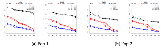
Figure 4. Plot of the RMSE and MRAB results of $\alpha$.

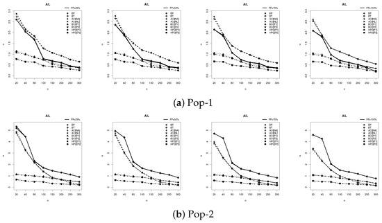
Figure 5. Plot of the AIL results of $\alpha$.

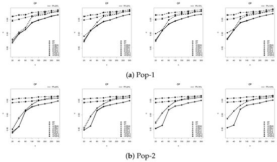
Figure 6. Plot of the CP results of $\alpha$.

7. Real Data Applications

This section examines two different real-world datasets, gathered from engineering and clinical domains, to achieve the following objectives: (a) to evaluate the flexibility, effectiveness, and applicability of the proposed DMB model in the real world; (ii) to highlight how the model’s inferential outputs can inform decisions in practical settings; and (iii) to show how its performance compares to eleven well-established existing discrete models. Table 6 provides the datasets used, which are as follows:

Table 6. Failure time points of liver cancer (Data-1) and shocks (Data-2).

Data-1
6	13	15	17	19	20	24	34
Data-2
2	3	6	6	7	9	9	10	10	11
12	12	12	13	13	13	15	16	16	18

Liver Cancer in Female Mice: 

This application examines the temporal patterns of mortality in female mice treated with continuously fed dietary concentrations of 2-acetylaminofluorene (2-AAF), a fluorene-derived compound known for its mutagenic and carcinogenic properties. Throughout the 18-month experimental period, mice were either systematically sacrificed at scheduled intervals, found dead, or euthanized upon reaching a moribund condition. Necropsies were conducted to determine the presence of hepatic neoplasms. The resulting data consist of time-to-death information and liver tumor incidence rates, offering a longitudinal perspective on chemically induced carcinogenesis in a controlled murine model. See, for more details, Zhang and Zelterman [24]. We henceforward refer to this dataset as Data-1.

Shocks Before Failure: 

This application investigates a dataset comprising twenty independent measurements, each reflecting the count of mechanical shocks sustained by a component before its functional breakdown. We henceforward refer to this dataset as Data-2. This dataset was first reported by Murthy et al. [25] and rediscussed later by Cordeiro et al. [26].

It is important to remember that the two datasets selected for this study, Data-1 from the medical domain and Data-2 from engineering, provide a diverse empirical basis, highlighting the proposed model’s ability to operate effectively across different application areas. Both datasets display complex real-world features, including discreteness and deviations from normality, which pose significant challenges for model validation. Table 7 presents the summary statistics for each dataset (Data-i, $i=1,2$), capturing key distributional characteristics such as the range (minimum and maximum), quartiles (${\mathsf{Q}}_i,i=1,2,3$), measures of central tendency (mean, mode), variability (standard deviation (SD)), and shape patterns (skewness and kurtosis). It indicates that Data-1 exhibits greater dispersion (SD = 8.229) and a right-skewed distribution (skewness = 0.474), whereas Data-2 shows lower variability (SD = 4.283) and mild left skewness (skewness = -0.359). Both datasets display mesokurtic tendencies (kurtosis < 3), indicating moderate tail behavior relative to the normal distribution.

Table 7. Statistical summary for datasets 1 and 2.

Minimum	Maximum	Quartiles			Mode	Mean	SD	Skewness	Kurtosis
		${\mathsf{Q}}_{\mathbf{1}}$	${\mathsf{Q}}_{\mathbf{2}}$	${\mathsf{Q}}_{\mathbf{3}}$
Data-1
6	34	14.5	18	21	6	18.500	8.229	0.474	2.995
Data-2
2	18	8.5	11.5	13	12	10.650	4.283	−0.359	2.497

To provide a comprehensive visualization of the data distribution, Figure 7 presents violin plots (in yellow color) for Data-i, $i=1,2$. These plots integrate boxplots (in red color) with kernel density estimates, thereby conveying both key summary statistics and the underlying distributional characteristics. Figure 7(left) shows greater variability and a positive skew, with at least one clear outlier, indicating more extreme values in the liver neoplasms dataset. Figure 7(right) shows a symmetric, unimodal distribution with moderate spread and no clear outliers.

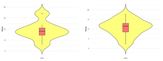
Figure 7. Violin diagrams of Data-1 (left) and Data-2 (right).

To infer the form of the hazard rate and to provide a graphical diagnostic for assessing the fit of lifetime distribution models in survival and reliability analysis, the scaled TTT-transform plots for Data-i, $i=1,2$ are shown in Figure 8. It reveals that both datasets 1 and 2 show an increasing failure rate, which is one of the DMB failure rates depicted in Figure 1.

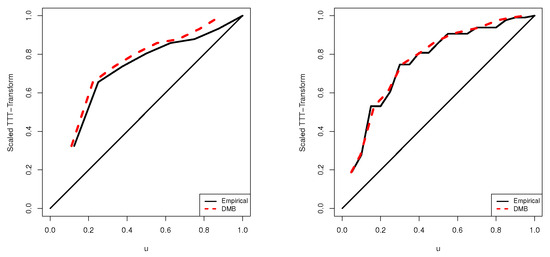
Figure 8. Scaled TTT curves of Data-1 (left) and Data-2 (right).

Now, to demonstrate the adaptability, flexibility, and effectiveness of the proposed DMB distribution, a comprehensive comparative analysis is conducted. Using each dataset summarized in Table 6, the goodness-of-fit performance of the DMB is evaluated against 11 popular discrete models from the literature; see Table 8.

Table 8. Eleven competing models of the DMB distribution.

Model	Symbol	Author(s)
Discrete Lindley	DL $\left(\alpha \right)$	Gómez-Déniz and Calderín-Ojeda [27]
Poisson	Pois $\left(\alpha \right)$	Poisson [28]
Geometric	Geom $\left(\alpha \right)$	Johnson et al. [29]
Discrete Gamma	DG $(\theta ,\alpha )$	Chakraborty and Chakravarty [30]
Negative Binomial	NB $(\theta ,\alpha )$	Johnson et al. [29]
Discrete Perks	DP $(\theta ,\alpha )$	Tyagi et al. [31]
Discrete Nadarajah–Haghighi	DNH $(\theta ,\alpha )$	Shafqat et al. [32]
Discrete Weibull	DW $(\theta ,\alpha )$	Nakagawa and Osaki [4]
Discrete Modified Weibull	DMW $(\theta ,\alpha ,\beta )$	Almalki and Nadarajah [33]
Exponentiated Discrete Weibull	EDW $(\theta ,\alpha ,\beta )$	Nekoukhou and Bidram [34]
Discrete Exponentiated-Chen	DEC $(\theta ,\alpha ,\beta )$	Alotaibi et al. [5]

To specify the most suitable model among the DMB and its competitors, a comprehensive analysis of model selection and goodness-of-fit criteria is employed, including the negative log-likelihood (NLL), Akaike information (AI), consistent AI (CAI), Bayesian information (BI), Hannan–Quinn information (HQI), and Kolmogorov–Smirnov (KS) statistics alongside its corresponding p-value. Table 9 reports the MLE (with its standard error (SE)) for each model parameter across all datasets under investigation. It also presents the estimated values of all metrics of model selection for each distribution listed in Table 8. Notably, the fitting outcomes provided in Table 9 show that the new DMB distribution demonstrates superior performance across all criteria, yielding the lowest values for each information-based metric. Table 9 also exhibits that the DMB model has the highest p-value with the lowest $\mathsf{KS}$ statistic compared to others. These findings stated that the proposed DMB model outperforms the competing alternatives; hence, it is the best choice when the entire Data-1 (or Data-2) is analyzed.

Table 9. Fitting summary for the DMB and its competitors from Data-$i,i=1,2$.

Model	$\mathit{\theta }$		$\mathit{\alpha }$		$\mathit{\beta }$		NLL	AI	CAI	BI	HQI	KS
	Est.	SE	Est.	SE	Est.	SE						Distance	p-Value
Data-1
DMB	-	-	-	-	278.90	80.210	27.498	56.997	57.663	57.076	56.461	0.1624	0.9623
DL	-	-	-	-	0.0296	0.0092	29.796	61.591	62.258	61.671	61.055	0.4649	0.0419
Pois	-	-	-	-	18.500	1.5207	31.747	65.493	66.160	65.573	64.958	0.1639	0.9593
Geom	-	-	-	-	0.0513	0.0177	31.555	65.109	65.776	65.189	64.573	0.3965	0.1208
DG	-	-	5.5278	2.6937	0.2909	0.1483	27.572	59.145	61.545	59.304	58.073	0.1661	0.9615
NB	-	-	18.499	2.7829	7.8745	5.7200	27.529	59.058	61.458	59.217	57.986	0.1636	0.9616
DP	-	-	0.0163	0.0248	0.2240	0.0739	27.524	59.048	61.448	59.207	57.977	0.1636	0.9620
DNH	-	-	0.0036	0.0034	10.886	10.316	29.772	63.544	65.944	63.703	62.472	0.3495	0.2228
DW	-	-	21.389	3.0194	2.6443	0.7161	27.515	59.030	61.430	59.189	57.958	0.1829	0.9106
DMW	0.5136	0.0683	35.378	48.658	0.7809	0.0682	34.235	74.470	80.470	74.708	72.863	0.4674	0.0402
EDW	2.4514	1.9968	1.6490	0.5498	0.9882	0.0237	27.516	61.032	67.032	61.270	59.424	0.1644	0.9583
DEC	4.1581	7.2790	0.4001	0.1434	0.0793	0.1828	27.502	60.963	66.963	61.201	59.356	0.1676	0.9517
Data-2
DMB	-	-	-	-	94.417	17.264	57.729	117.459	117.681	118.454	117.653	0.1166	0.9486
DL	-	-	-	-	0.0511	0.0101	63.628	129.257	129.479	130.252	129.451	0.4248	0.0015
Pois	-	-	-	-	10.650	0.7297	59.876	121.751	121.974	122.747	121.946	0.2263	0.2572
Geom	-	-	-	-	0.0858	0.0183	68.222	138.444	138.666	139.440	138.639	0.3665	0.0093
DG	-	-	5.2320	1.6288	0.4692	0.1530	58.824	121.649	122.355	123.640	122.038	0.1237	0.9195
NB	-	-	10.6510	0.9870	12.849	9.8657	58.113	120.226	120.932	122.217	120.615	0.1922	0.4507
DP	-	-	0.0112	0.0109	0.3987	0.0767	57.793	118.256	118.962	120.247	118.645	0.1635	0.6591
DNH	-	-	0.0037	0.0026	18.008	12.512	63.249	130.498	131.204	132.489	130.886	0.3065	0.0467
DW	-	-	12.4731	0.9743	2.9995	0.5589	57.791	118.026	118.732	120.017	118.415	0.1223	0.9257
DMW	1.2631	0.0636	1.5825	2.3660	0.9920	0.0094	57.756	119.117	120.617	122.104	119.700	0.1723	0.5924
EDW	1.4646	0.4894	2.1818	0.2647	0.9944	0.0042	57.822	121.245	122.745	124.232	121.828	0.1917	0.4541
DEC	1.0002	0.3792	0.6406	0.0489	0.0059	0.0052	57.933	118.659	120.159	121.646	119.242	0.1547	0.7245

Goodness-of-fit visualization techniques serve as valuable diagnostic tools for evaluating the concordance between empirical data and a proposed theoretical distribution. For this purpose, in Figure 9, we demonstrate the superior performance of the DMB model through the application of three key graphical evaluation methods: (i) lines representing fitted probability mass lines with data histograms, (ii) fitted reliability function lines, and (iii) probability–probability (PP) lines.

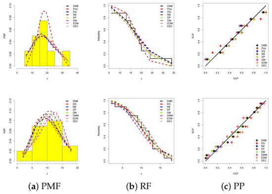
Figure 9. Data visualizations of the DMB and its competitors Data-1 (top) and Data-2 (bottom).

Figure 9 confirms the numerical outcomes presented in Table 9, collectively supporting the conclusion that the proposed DMB model demonstrates superior fitting performance compared to several existing statistical models, both classical and newly developed.

To assess the performance of the estimators for the DMB ($\alpha$) parameter—derived via MLE, bootstrap methods (with 10,000 replications), and Bayesian inference—different type-II right-censored samples, corresponding to different FP% levels, are generated from each dataset provided in Table 6. For each sample $\mathbb{S}\left[i\right]$ (where $i=1,2,3$), both point estimates (along with their SEs) and 95% interval estimates (along with their interval widths (IWs)) of $\alpha$ are computed and presented in Table 10. A comparative analysis of Table 10 reveals that the Bayesian point estimators consistently exhibit smaller SEs than those obtained through frequentist (likelihood-based) methods, indicating greater estimation precision within the Bayesian framework. Furthermore, Table 10 shows that the Bayesian interval estimates, based on BCI (or HPD) interval method, consistently yield narrower IWs compared to those developed from frequentist intervals (including BP/BT and ACI[NA]/ACI[NL]). It is also observed that as the FP% increases, both the SEs and IWs associated with the estimation of $\alpha$ tend to decrease, reflecting improved estimator efficiency. The utility of the proposed methodology is further demonstrated through its application to two widely used real-world datasets collected from distinct scientific domains, thereby affirming its practical relevance.

Table 10. The point and 95% interval estimates of $\alpha$ from Data-$i,i=1,2$.

n [FP%]	MLE		BP			ACI [NA]			BCI
	Bayes		BT			ACI [NL]			HPD
	Est.	SE	Low.	Upp.	IW	Low.	Upp.	IW	Low.	Upp.	IW
Data-1
8 [50%]	271.007	11.863	252.044	284.234	32.1898	247.755	294.259	46.5032	267.053	274.960	7.9071
	270.977	2.0138	248.181	271.801	23.6192	248.725	295.285	46.5603	267.013	274.905	7.8918
8 [75%]	245.670	2.8773	230.781	256.662	25.8812	240.031	251.309	11.2787	241.732	249.637	7.9049
	245.650	2.0064	248.181	271.801	23.6192	240.095	251.375	11.2797	241.646	249.531	7.8851
Data-2
20 [50%]	106.491	8.3886	66.0533	152.951	86.8975	90.0492	122.932	32.8827	96.705	115.986	19.281
	106.298	4.9364	248.181	271.801	23.6192	91.2555	124.269	33.0135	96.827	116.080	19.253
20 [75%]	98.1909	11.863	71.9970	140.884	68.8868	74.9393	121.443	46.5032	88.548	107.581	19.033
	98.0135	4.8447	248.181	271.801	23.6192	77.4873	124.426	46.9390	88.474	107.462	18.988

A main issue in utilizing the MCMC methodology is verifying that the simulation has achieved satisfactory convergence. To this end, Figure 10 displays both the trace plots and posterior density estimates for the parameter $\alpha$. Each panel includes the posterior mean (represented by a solid red line) and the 95% BCI bounds (shown as dashed red lines), providing a visual assessment of convergence and the underlying distributional characteristics. The plotted outcomes suggest that the proposed M-H approach attains reliable convergence, with the resulting DMB posterior distributions exhibiting approximate symmetry across samples from Data-$i,i=1,2$. Additionally, Table 11 presents a comprehensive summary of key statistics for $\alpha$, derived from 30,000 iterations of the MCMC algorithm. Notably, the results in Table 11 support the numerical findings reported in Table 10 and behave similarly to the facts shown in Figure 10.

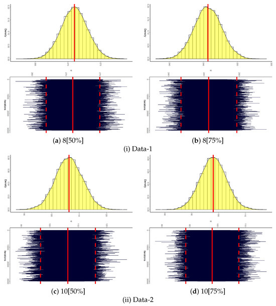
Figure 10. Convergence MCMC diagrams of $\alpha$ from Data-$i,i=1,2$.

Table 11. Statistics for 30,000 MCMC iterations of $\alpha$ from Data-$i,i=1,2$.

n [FP%]	Mean	Mode	Quartiles			SD	Skewness
			${\mathsf{Q}}_{\mathbf{1}}$	${\mathsf{Q}}_{\mathbf{2}}$	${\mathsf{Q}}_{\mathbf{3}}$
Data-1
8 [50%]	270.977	267.860	269.628	270.973	272.317	2.0136	0.0213
8 [75%]	245.650	238.490	244.296	245.634	247.012	2.0064	0.0120
Data-2
20 [50%]	106.298	103.679	102.968	106.277	109.629	4.9327	0.0016
20 [75%]	98.0135	95.2265	94.7406	97.9918	101.264	4.8415	0.0379

In summary, from the data analysis of Data-$i,i=1,2$, it is clear that the proposed one-parameter DMB distribution exhibits excellent statistical properties, providing robust performance, high flexibility, and superior empirical fit compared to classical and modern discrete models. Its adaptability to diverse domains and reliable inference capabilities (especially within a Bayesian framework) underscore its value as a practical and theoretically sound tool for modeling real-world discrete data.

8. Conclusions

A novel one-parameter discrete probability called the discrete Maxwell–Boltzmann distribution was proposed in this article. It is a viable substitute for a few well-known discrete distributions. The DMB distribution’s mathematical characteristics are shown. Bayesian and maximum likelihood techniques are used to estimate the parameter. To compare these approaches, thorough simulation results are performed. Based on our discussion, the Bayes method outperforms its rival, the maximum likelihood approach, for point estimating techniques. Overall, the HPD (or BCI) interval approach combined with Bayesian estimation works very well for parameter inference in both complete and incomplete (censoring) frameworks, producing accurate and dependable results even when the data are incomplete. Beyond its theoretical development, the discrete MB model was shown to be highly adaptable to real-world count data exhibiting specific dispersion structures. Two distinct datasets were analyzed, one based on liver cancer in female mice and the other based on the count of mechanical shocks sustained, to demonstrate its superior goodness-of-fit over existing competing models, thereby confirming its flexibility and making it the optimal option. The work also highlighted potential applications in reliability analysis, actuarial science, and information theory, opening avenues for further interdisciplinary research.

References

- Alizadeh, M.; Khan, M.N.; Rasekhi, M.; Hamedani, G.G. A new generalized modified Weibull distribution. Stat. Optim. Inf. Comput. 2021, 9, 17–34. [Google Scholar] [CrossRef]
- Keefer, D.L.; Bodily, S.E. Three–point approximations for continuous random variables. Manag. Sci. 1983, 29, 595–609. [Google Scholar] [CrossRef]
- Miller, A.C., III; Rice, T.R. Discrete approximations of probability distributions. Manag. Sci. 1983, 29, 352–362. [Google Scholar] [CrossRef]
- Nakagawa, T.; Osaki, S. The discrete Weibull distribution. IEEE Trans. Reliab. 2009, 24, 300–301. [Google Scholar] [CrossRef]
- Alotaibi, R.; Rezk, H.; Park, C.; Elshahhat, A. The discrete exponentiated–Chen model and its applications. Symmetry 2023, 15, 1278. [Google Scholar] [CrossRef]
- Chesneau, C.; Gillariose, J.; Joseph, J.; Tyagi, A. New discrete trigonometric distributions: Estimation with application to count data. Int. J. Model. Simul. 2024, 1–16. [Google Scholar] [CrossRef]
- Lai, C.D. Issues concerning constructions of discrete lifetime models. Qual. Technol. Quant. Manag. 2013, 10, 251–262. [Google Scholar] [CrossRef]
- Chakraborty, S. Generating discrete analogues of continuous probability distributions–A survey of methods and constructions. J. Stat. Distrib. Appl. 2015, 2, 6. [Google Scholar] [CrossRef]
- Afify, A.Z.; Ahsan-ul-Haq, M.; Aljohani, H.M.; Alghamdi, A.S.; Babar, A.; Gómez, H.W. A new one—Parameter discrete exponential distribution: Properties, inference, and applications to COVID-19 data. J. King Saud-Univ. -Sci. 2022, 34, 102199. [Google Scholar] [CrossRef]
- Augusto Taconeli, C.; Rodrigues de Lara, I.A. Discrete Weibull distribution: Different estimation methods under ranked set sampling and simple random sampling. J. Stat. Comput. Simul. 2022, 92, 1740–1762. [Google Scholar] [CrossRef]
- Roy, D.; Gupta, R.P. Characterizations and model selections through reliability measures in the discrete case. Stat. Probab. Lett. 1999, 43, 197–206. [Google Scholar] [CrossRef]
- Roy, D.; Ghosh, T. A new discretization approach with application in reliability estimation. IEEE Trans. Reliab. 2009, 58, 456–461. [Google Scholar] [CrossRef]
- Bebbington, M.; Lai, C.D.; Wellington, M.; Zitikis, R. The discrete additive Weibull distribution: A bathtub-shaped hazard for discontinuous failure data. Reliab. Eng. Syst. Saf. 2012, 106, 37–44. [Google Scholar] [CrossRef]
- Haj Ahmad, H.; Elshahhat, A. A new Hjorth distribution in its discrete version. Mathematics 2025, 13, 875. [Google Scholar] [CrossRef]
- Peckham, G.D.; McNaught, I.J. Applications of Maxwell–Boltzmann distribution diagrams. J. Chem. Educ. 1992, 69, 554. [Google Scholar] [CrossRef]
- Rowlinson, J.S. The Maxwell—Boltzmann distribution. Mol. Phys. 2005, 103, 2821–2828. [Google Scholar] [CrossRef]
- Roy, D. The discrete normal distribution. Commun. Stat. Methods 2003, 32, 1871–1883. [Google Scholar] [CrossRef]
- Roy, D. Discrete Rayleigh distribution. IEEE Trans. Reliab. 2004, 53, 255–260. [Google Scholar] [CrossRef]
- Krishna, H.; Pundir, P. Discrete Maxwell distribution. InterStat 2007, 1–15. Available online: http://interstat.statjournals.net/YEAR/2007/articles/0711003.pdf (accessed on 1 August 2025).
- Henningsen, A.; Toomet, O. maxLik: A package for maximum likelihood estimation in R. Comput. Stat. 2011, 26, 443–458. [Google Scholar] [CrossRef]
- Lawless, J.F. Statistical Models and Methods for Lifetime Data; John Wiley and Sons: Hoboken, NJ, USA, 2011. [Google Scholar]
- Meeker, W.Q.; Escobar, L.A. Statistical Methods for Reliability Data; John Wiley and Sons: New York, NY, USA, 2014. [Google Scholar]
- Chernick, M.R.; LaBudde, R.A. An Introduction to Bootstrap Methods with Applications to R; John Wiley and Sons: Hoboken, NJ, USA, 2014. [Google Scholar]
- Zhang, H.; Zelterman, D. Binary Regression for Risks in Excess of Subject-Specific Thresholds. Biometrics 1999, 55, 1247–1251. [Google Scholar] [CrossRef]
- Murthy, D.N.P.; Xie, M.; Jiang, R. Weibull Models; John Wiley: Hoboken, NJ, USA, 2004. [Google Scholar]
- Cordeiro, G.M.; Lima, M.D.C.S.; Cysneiros, A.H.; Pascoa, M.A.; Pescim, R.R.; Ortega, E.M. An extended Birnbaum–Saunders distribution: Theory, estimation, and applications. Commun. Stat. Theory Methods 2016, 45, 2268–2297. [Google Scholar] [CrossRef]
- Gómez–Déniz, E.; Calderín–Ojeda, E. The discrete Lindley distribution: Properties and applications. J. Stat. Comput. Simul. 2011, 81, 1405–1416. [Google Scholar] [CrossRef]
- Poisson, S.D. Recherches sur la Probabilité des Jugements en Matière Criminelle et en Matière Civile: Précédées des Règles Générales du Calcul des Probabilités; Bachelier: Paris, France, 1837. [Google Scholar]
- Johnson, N.L.; Kemp, A.W.; Kotz, S. Univariate Discrete Distributions; John Wiley and Sons: New York, NY, USA, 2005. [Google Scholar]
- Chakraborty, S.; Chakravarty, D. Discrete gamma distributions: Properties and parameter estimations. Commun. Stat. Theory Methods 2012, 41, 3301–3324. [Google Scholar] [CrossRef]
- Tyagi, A.; Choudhary, N.; Singh, B. A new discrete distribution: Theory and applications to discrete failure lifetime and count data. J. Appl. Probab. Statist. 2020, 15, 117–143. [Google Scholar]
- Shafqat, M.; Ali, S.; Shah, I.; Dey, S. Univariate discrete Nadarajah and Haghighi distribution: Properties and different methods of estimation. Statistica 2020, 80, 301–330. [Google Scholar]
- Almalki, S.J.; Nadarajah, S. A new discrete modified Weibull distribution. IEEE Trans. Reliab. 2014, 63, 68–80. [Google Scholar] [CrossRef]
- Nekoukhou, V.; Bidram, H. The exponentiated discrete Weibull distribution. Sort 2015, 39, 127–146. [Google Scholar]
Disclaimer/Publisher’s Note: The statements, opinions and data contained in all publications are solely those of the individual author(s) and contributor(s) and not of MDPI and/or the editor(s). MDPI and/or the editor(s) disclaim responsibility for any injury to people or property resulting from any ideas, methods, instructions or products referred to in the content. |
© 2025 by the authors. Licensee MDPI, Basel, Switzerland. This article is an open access article distributed under the terms and conditions of the Creative Commons Attribution (CC BY) license (https://creativecommons.org/licenses/by/4.0/).