Abstract
In recent years, machine learning (ML) techniques have gained significant attention in time series classification tasks, particularly in industrial applications where early detection of abnormal conditions is crucial. This study proposes an intelligent monitoring framework based on a multimodal convolutional neural network (CNN) to classify normal and abnormal copper ion (Cu2+) concentration states in the etching process in the printed circuit board (PCB) industry. Maintaining precise control Cu2+ concentration is critical in ensuring the quality and reliability of the etching processes. A sliding window approach is employed to segment the data into fixed-length intervals, enabling localized temporal feature extraction. The model fuses two input modalities—raw one-dimensional (1D) time series data and two-dimensional (2D) recurrence plots—allowing it to capture both temporal dynamics and spatial recurrence patterns. Comparative experiments with traditional machine learning classifiers and single-modality CNNs demonstrate that the proposed multimodal CNN significantly outperforms baseline models in terms of accuracy, precision, recall, F1-score, and G-measure. The results highlight the potential of multimodal deep learning in enhancing process monitoring and early fault detection in chemical-based manufacturing. This work contributes to the development of intelligent, adaptive quality control systems in the PCB industry.
Keywords:
multimodal convolutional neural network (CNN); printed circuit board; etching process; recurrence plot MSC:
37M10
1. Introduction
In recent years, machine learning (ML) techniques have gained significant attention in time series classification tasks [1,2,3]. One widely adopted approach involves segmenting continuous data streams using a sliding window method [4,5,6,7,8], which enables the extraction of fixed-length sequences for input into classification models. This technique effectively captures temporal patterns while accommodating data streams of varying lengths.
This paper presents the application of ML techniques to classify etchant concentration levels in the etching process in the printed circuit board (PCB) industry. PCB manufacturing involves complex chemical processes, where maintaining precise control over solution conditions is critical in ensuring product quality. Among these processes, chemical etching is particularly sensitive to the concentration of etchant, which directly affects the etch rate, uniformity, and surface integrity. Deviations in the etchant’s concentration can result in defects such as under-etching, over-etching, or pattern distortion, ultimately compromising the functionality of the final product.
This study investigates a micro-etching process used in the treatment of PCBs, with a particular emphasis on sodium persulfate (SPS) as the primary etching agent. The concentration of copper ions (Cu2+) is a by-product and serves as an indicator of SPS consumption during the etching process. Traditional monitoring methods rely on physical sensors and threshold-based controls, which often lack the sensitivity to detect subtle fluctuations or complex temporal patterns in Cu2+ concentration during the PCB etching process. The key challenge, therefore, is accurately identifying abnormal etching conditions from complex, time-dependent data. To address these limitations, this study proposes an intelligent monitoring framework for real-time tracking and evaluation of Cu2+ concentration. The concentration data are collected as time series and analyzed using a sliding window approach to capture temporal dynamics. The goal of the monitoring system is to accurately classify normal and abnormal etching conditions, enabling timely intervention and adaptive process control.
Recent advances in multimodal deep learning have demonstrated that fusing complementary data sources can significantly improve model performance [9,10]. Inspired by these approaches, this study proposes a multimodal convolutional neural network (CNN) that integrates information from both raw one-dimensional (1D) time series data and their corresponding two-dimensional (2D) recurrence plots, capturing both temporal and spatial features [11,12,13]. This architecture enhances the model’s ability to differentiate between normal operating conditions and various abnormal states that may reflect concentration deviations or process instabilities. The multimodal CNN is trained to perform multi-class classification, providing actionable insights for real-time diagnosis and process correction.
To evaluate the performance of the proposed model, we conduct a comparative study using various traditional and deep learning classifiers. The experimental results demonstrate that the multimodal CNN outperforms baseline models in terms of accuracy, precision, recall, F1-score, and G-measure, offering a reliable solution for real-time monitoring and early fault detection in PCB etching. The ability to accurately classify the etchant’s concentration states not only enables timely corrective actions but also contributes to the development of intelligent, human-in-the-loop manufacturing systems capable of autonomous condition monitoring and data-driven decision-making [14,15].
The remainder of this paper is organized as follows: Section 2 reviews related work on sliding window techniques and machine learning approaches for multimodal classification across various domains. Section 3 describes the materials and methods used in this study, including data collection, preprocessing, and the design of the proposed multimodal CNN model. Section 4 details the experimental setup, covering implementation specifics and the training procedure. Section 5 presents the classification results, compares the performance of different models, and provides a comprehensive analysis of the findings. Finally, Section 6 concludes the paper and outlines potential directions for future research and practical deployment in industrial environments.
2. Related Work
Time series classification using ML has shown strong potential in capturing dynamic behaviors of process variables. Sliding window segmentation [4,5,6,7,8] is a widely used technique in this domain, where continuous time series data are partitioned into fixed-length segments for model training and inference. This approach enables localized temporal features to be extracted and improves the adaptability of ML models to real-time data streams.
CNNs have been successfully applied in time series classification due to their ability to learn hierarchical features from local patterns [1,2]. Recent studies [11,12,13] have extended CNN architectures to handle multimodal inputs, combining 1D temporal signals with 2D representations such as recurrence plots (RPs), spectrograms, or Gramian angular fields (GAFs). These multimodal CNNs can learn complementary features that are not fully captured by a single data type. Typically, separate CNN branches are used to extract modality-specific features, which are then fused at an appropriate stage (early, late, or hybrid fusion) to form a joint representation for classification.
Ranipa et al. [16] proposed a multimodal CNN fusion architecture for classifying heart sound signals. Their approach involves extracting both general frequency features and Mel-domain features from raw heart sound data to train multimodal CNN. CNNs have also recently been applied to the task of activity recognition [17,18,19,20].
In the context of Alzheimer’s disease (AD), multimodal approaches have been widely explored for diagnosis and monitoring, leveraging complementary information from diverse data sources to enhance model accuracy and robustness [21,22,23,24]. Similarly, multimodal deep learning has been increasingly applied to brain tumor grade classification, benefiting from the integration of multiple imaging modalities [25,26,27].
In a wider context, multimodal deep learning has gained increasing attention in time series classification, due to its capacity to combine complementary information from different data modalities. Previous studies [28,29,30,31] have investigated the fusion of heterogeneous inputs—such as raw signals, spectrograms, and recurrence plots—to jointly capture temporal and spatial features for improved classification performance.
Several review studies have comprehensively summarized the applications of multimodal CNNs in industrial process monitoring, diagnostics, and pattern recognition [32,33]. For detailed comparisons and analyses of various network architectures, see [34,35,36].
This study builds upon these foundations by proposing a multimodal CNN-based framework for real-time classification of etchant concentration levels in the PCB etching process. By combining raw time series data with recurrence plot representations using a sliding window mechanism, the model captures both temporal dynamics and spatial patterns.
3. Materials and Methods
In the PCB manufacturing process, precise control of the etching solution’s chemical concentration is essential in ensuring product quality and process reliability. Fluctuations in concentration can lead to surface defects, reduced yield, and increased operational downtime. Traditional monitoring methods often rely on manual sampling or threshold-based alarms, which may be insufficient for detecting subtle or early-stage abnormalities. To address these limitations, this study proposes an intelligent monitoring framework that leverages deep learning techniques to automatically detect and classify abnormal concentration patterns in real time.
As shown in Figure 1, the proposed framework combines 1D residual time series data and 2D recurrence plots within a multimodal CNN architecture. By capturing both the temporal and spatial characteristics of the etching process, the framework enables accurate and timely detection of abnormal concentration states, thereby supporting process stability and quality assurance.
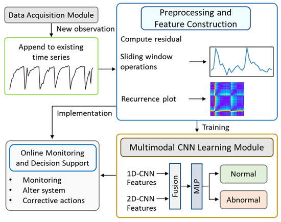
Figure 1.
Intelligent monitoring framework for Cu2+ concentration in the etching solution. The framework integrates multimodal data processing, feature extraction, and classification to enable real-time monitoring and early detection of abnormal process states.
The core components of the framework can be outlined as follows:
- Data acquisition moduleReal-time sensor measurements of etchant+ concentration are collected at regular intervals, forming a time series that captures the dynamic behavior of the etching solution.
- Preprocessing and feature constructionA reference pattern representing the normal operating state is established. In this study, a reference normal pattern can be established using domain knowledge. In the context of PCB etching, process experts can define expected Cu2+ concentration ranges based on process specifications, historical experience, or industry standards. In our study, the data are aligned with the replenishment cycle, making it essential to preserve the original sequence length. Therefore, missing or null values were not removed but imputed. Residual values are computed by comparing the observed time series against this reference. These residuals are then segmented using a sliding window approach. Each segment is transformed into two parallel data representations: the original 1D residual time series and a 2D recurrence plot, which encodes temporal recurrences and state transitions. The 1D residual time series were standardized using Z-score normalization, and the 2D recurrence plot features were scaled to [0, 1]. Scaling parameters were computed from the training set and applied to the test set to prevent information leakage. These preprocessed features were input into the multimodal CNN, where separate streams were fused in a late fusion stage, ensuring effective integration and model convergence.
- Multimodal deep learning modelA multimodal convolutional neural network is employed to classify the solution concentration status as either normal or abnormal. A 1D-CNN branch extracts temporal features from the residual time series. A 2D-CNN branch processes the recurrence plots to extract spatial recurrence patterns. The outputs from both branches are concatenated and passed through dense layers for final classification.
- Model training and evaluationThe model is trained on labeled data containing both normal and abnormal concentration patterns. We evaluated model performance using the accuracy, precision, recall, F1-score, and G-measure. The G-measure is calculated as the square root of the product of sensitivity and specificity. While the F1-score balances precision and recall, emphasizing the model’s ability to correctly identify positive instances, the G-measure—defined as the geometric mean of recall and specificity—captures performance across both positive and negative classes. This makes it particularly valuable in imbalanced classification scenarios. A large discrepancy between the F1-score and G-measure indicates class-dependent behavior, suggesting that the confusion matrix should be examined to determine which class is being favored or overlooked.
- Online monitoring and decision supportOnce deployed, the framework continuously receives incoming sensor data, performs real-time classification, and triggers alerts when abnormal concentration trends are detected. This enables operators to take timely corrective actions, such as replenishing the etching solution or inspecting the chemical delivery mechanism.
The components outlined above are discussed in detail in the following subsections.
3.1. Process Description and Data Collection
This study investigates a micro-etching process employed in the treatment of PCBs, with a particular focus on sodium persulfate (SPS) as the primary etching agent. SPS is a strong oxidizing agent commonly used to etch copper by reacting with metallic copper (Cu0) on the PCB surface, converting it into soluble copper ions (Cu2+). The process serves two key purposes: cleaning the oxidized copper surface to improve electrical conductivity and roughening the surface to increase the electroplating area and enhance adhesion.
During etching, the Cu2+ concentration in the solution gradually increases. Elevated Cu2+ levels can reduce the etching rate and diminish the oxidizing efficiency of SPS. As such, monitoring Cu2+ concentration provides an indirect yet effective means of tracking SPS consumption and the overall progress of the etching process. Deviations from the expected Cu2+ concentration trend may signal underlying abnormalities in the system. Therefore, maintaining proper control over Cu2+ concentration is crucial in ensuring stable and consistent etching performance. The potential causes of fluctuations in Cu2+ concentration are discussed below.
- A sudden increase in Cu2+ concentration may result from a higher number of boards being processed. Currently, the dosing formula does not account for the actual board count. The countermeasure is to revise the dosing formula.
- A sudden drop in Cu2+ concentration may be caused by improperly installed rollers, which allow water from the upstream tank to be carried into the micro-etching tank along with the boards, thereby diluting the Cu2+ concentration. The countermeasure is to inspect whether the rollers are operating smoothly or exhibit any wobbling.
- If the rate of Cu2+ concentration increase changes, one possible reason is a decrease in the number of boards being processed, which slows down the rate of Cu2+ increase. The countermeasure is to revise the dosing formula. If the board quantity has not decreased, then a possible reason could be a malfunction in the electrodes. In this case, the recommended countermeasure is to inspect whether the electrodes are functioning properly.
In the studied etching process, a new batch of solution is prepared every 14 time units, and the solution’s concentration varies over time. Figure 2 presents the time series plot of Cu2+ concentration. To improve the detection of abnormalities in Cu2+ concentration, the client requested the implementation of an I-MR control chart combined with the Western Electric rules [37]. It is evident that the data do not follow a normal distribution. When conventional control charts are applied, they tend to produce an excessive number of false alarms (Type I errors). Conversely, they are often ineffective at detecting true abnormalities in solution concentration (Type II errors).

Figure 2.
Time series plots of Cu2+ concentration. Subplots (a,c–e,g) correspond with normal conditions, showing stable trends, whereas (b,f) depict abnormal conditions with irregular fluctuations or sudden deviations, indicating potential process instabilities.
The dataset used in this work was obtained from an operational PCB manufacturing process, where Cu2+ concentrations (grams per liter, g/L) were continuously measured under both normal and abnormal conditions. After collecting Cu2+ concentration data, representative samples of the normal operating state are first identified based on expert judgment from field personnel. These samples are then used to establish a reference pattern, representing the standard concentration profile. The observed data is compared against this reference to calculate residual values, which highlight deviations from normal behavior and aid in extracting key pattern features, thereby improving classification accuracy.
A sliding window approach was used to segment the residual time series into fixed-length overlapping windows of size samples. Each extracted segment was treated as an independent input sample for classification. Figure 3 illustrates the sliding window approach. The data instance was labeled based on expert annotations and process logs, resulting in a multi-class classification problem.
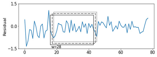
Figure 3.
Sliding window approach for real-time monitoring. With a stride of 1, each new data point is incorporated into the analysis, enabling timely detection of abnormal Cu2+ concentration patterns.
In this study, the window stride was set to 1 in order to enable real-time monitoring. Using a stride of 1 ensures that every new data point is incorporated into the analysis without delay, allowing the model to capture subtle fluctuations in Cu2+ concentration and promptly detect abnormal patterns. While this choice increases data redundancy, it is necessary for achieving high temporal resolution in real-time classification. In practical applications, when a new Cu2+ observation is collected, it is appended to the existing time series to generate a new sliding window, which is then fed into the multimodal CNN model for analysis and classification.
3.2. Recurrence Plot
The recurrence plot (RP), introduced by Eckmann et al. [38], is a non-linear data analysis technique used to visualize the structure of time series data and uncover hidden patterns. It offers meaningful and interpretable insights into the temporal dynamics of complex systems. Recurrence refers to the phenomenon where certain system states exhibit similar or repetitive characteristics over time.
An RP is a two-dimensional visualization method that illustrates the recurrence of states within a dynamical system [38]. It is commonly used for the qualitative assessment of time series behavior and to track how the similarity between subsequences evolves over time [39]. In time series analysis, RPs reveal temporal dependencies and structural patterns that may not be evident in the original one-dimensional signal. For classification tasks, recurrence plots are generated from sliding windows of the time series and used as two-dimensional inputs for the classification model.
The first step in generating a recurrence plot is to reconstruct the phase space of the time series. For a time series of length , the reconstructed phase space can be represented as follows:
where is the embedded dimensions, and is the delay time. The subsequence is referred to as the th state in the phase space and is also known as trajectory. Each subsequence represents a distinct point in the phase space trajectory.
where , is the threshold distance, and denotes the Euclidean norm. Here, denotes a Heaviside step function, which returns 1 for positive arguments and 0 for negative ones. In this approach, if two extracted trajectories, and , are sufficiently close, the corresponding entry is set to 1; otherwise, it is set to 0. The RP plot is a graphical representation of the matrix R, where the total number of states determines the size of the recurrence plot, resulting in an image. Depending on whether or not a threshold was selected, the resulting image could be binary or grayscale. Equation (3), which uses a fixed threshold, produces a binary image. To extract more detailed information from RP images, this study adopts an un-threshold technique as described in [40]. The recurrence matrix is defined as follows:
Iwanski and Bradley [41] conducted a systematic analysis of the structures represented by recurrence plots and concluded that RPs constructed with different embedding dimensions convey equivalent information, rendering higher-dimensional phase spaces unnecessary. Accordingly, the embedding dimension was set to 1 in this study. To preserve a larger RP image size and retain essential features, a window size of = 28 was adopted in this study. The choice of 28 is based on both domain knowledge of the PCB etching process and empirical performance evaluation. In our production setting, the etchant replenishment cycle is approximately 14 time units. Setting the window to 28 captures two consecutive replenishment cycles, which is important for distinguishing between normal variations and emerging abnormal patterns. Figure 4 shows the texture images generated through recurrence reconstruction of the chemical solution concentration patterns.
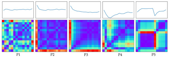
Figure 4.
Residual patterns and their corresponding recurrence plots with a sliding window size of 28. The recurrence plots reveal spatial recurrence structures that complement the temporal information in the residuals, enabling the detection of subtle differences between normal and abnormal Cu2+ concentration states.
3.3. Multimodal CNN Architecture
The proposed classification model is a multimodal convolutional neural network (CNN) consisting of two parallel branches. The first branch, a 1D-CNN [42], processes the raw time series signals using convolutional, ReLU activation and pooling layers to extract temporal features. The second branch, a 2D-CNN, processes recurrence plots through 2D convolutional and max-pooling layers to extract spatial features.
In multimodal CNNs, fusion methods define how features from different modalities are combined to create a joint representation for downstream tasks [43,44,45]. Common strategies include early fusion, intermediate fusion, and late fusion, with the choice depending on the specific task and characteristics of the data [44]. Owing to its simplicity, late fusion remains the predominant approach in many state-of-the-art multimodal applications [43]. In this work, we employ late fusion with simple concatenation, enabling independent feature learning for each modality while preserving complete feature information with minimal computational overheads.
The main reasons for selecting late fusion were its simplicity and its ability to preserve the independence of temporal and spatial features prior to integration, which has been reported as beneficial in multimodal CNN architectures [46]. Pereira et al. [46] also noted that when large training sets are available, early fusion tends to be the optimal choice, whereas with limited training data, late fusion is more appropriate.
In late fusion with a simple concatenation strategy, the outputs from both branches are merged and passed through fully connected layers, followed by a Softmax activation function for multi-class classification. Figure 5 depicts the architecture of the multimodal CNN, which processes both 1D and 2D inputs through parallel convolutional branches. The feature representations extracted from the 1D-CNN and 2D-CNN are concatenated into a unified feature vector, which is subsequently fed into a multi-layer perceptron (MLP) classifier for final prediction.
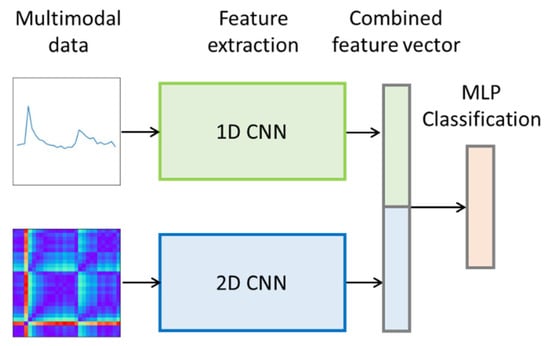
Figure 5.
Basic architecture of the proposed multimodal CNN. The network integrates 1D time series and 2D recurrence plot inputs using late fusion with simple concatenation. This strategy preserves the independence of temporal and spatial features before integration, enabling the model to exploit complementary information from both modalities and thereby improving classification performance.
4. Experimental Setup and Implementation
Data Description and Preprocessing
Figure 6 illustrates the distinct residual patterns associated with normal and abnormal conditions, as analyzed in this study. Figure 6a illustrates the standard concentration pattern, serving as the reference. Figure 6b displays the time series of concentration values under normal conditions, referred to as Pattern 1 (P1). Figure 6g shows the residuals obtained by subtracting P1 from the standard pattern, characterized by fluctuations around zero.
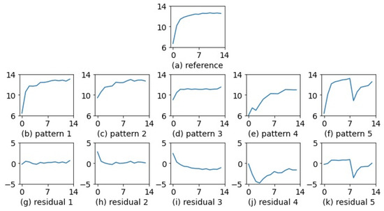
Figure 6.
Residual patterns observed under normal and abnormal conditions. Normal states exhibit stable residual fluctuations, whereas abnormal conditions show irregular or amplified deviations, indicating disturbances in Cu2+ concentration and potential process instabilities.
Figure 6c depicts Pattern 2 (P2), which results from incomplete preparation of the bath solution, leading to an initially high concentration value. The corresponding residuals in Figure 6h, obtained by subtracting P2 from the standard pattern, exhibit one particularly large deviation, with the remaining values fluctuating around zero.
Figure 6d illustrates Pattern 4 (P3), which is also caused by incomplete bath preparation—resulting in an initially high concentration—followed by subsequent changes that deviate more significantly from the normal state. Figure 6i displays the residuals obtained by subtracting P3 from the standard pattern, characterized by one particularly large deviation and the remaining values being predominantly below zero.
Figure 6e presents Pattern 4 (P4), which results from irregular fluctuations in concentration values. The corresponding residuals in Figure 6j, obtained by subtracting P4 from the standard pattern, consistently fall below zero and exhibit irregular variations.
Figure 6f illustrates Pattern 5 (P5), caused by a malfunction in the automatic chemical delivery mechanism, leading to a sudden drop in concentration at a specific time point. Figure 6k shows the residuals obtained by subtracting P5 from the standard pattern, which are marked by a sharp decline at that particular point in time.
A total of 1500 data instances were collected, with slight variations in the number of samples per class: 346 for P1, 331 for P2, 337 for P3, 343 for P4, and 142 for P5. The dataset was partitioned into training and testing sets in a 2:1 ratio using stratified sampling to maintain class distribution. To objectively evaluate the effectiveness of various classification models in a multi-class setting, no adjustments were made to address class imbalance. Oversampling can lead to overfitting by replicating minority class samples or generating synthetic instances that may not reflect the true data distribution, while downsampling risks discarding informative samples from the majority class. Both methods can also distort the natural class proportions, which is undesirable when the model is expected to operate under real-world conditions. Instead, we relied on the model’s learning capacity to mitigate the effects of imbalance without altering the original data distribution. However, evaluation metrics beyond accuracy—such as recall, precision, F1-score, and G-measure—were also considered. To reduce the influence of data partitioning variability, the experiments were repeated 10 times with different training–testing splits, and the average performance across these runs was reported.
Figure 6 illustrates the residual variations within a single etching cycle under normal and various abnormal conditions. However, in practical applications, analysis is performed using a sliding window approach. As the window moves over time, the arrangement of features within the window changes, which increases the complexity of classification. Using Pattern P3 as an example, Figure 7 illustrates that critical features may appear at different positions within an analysis window. Therefore, the classification model should be able to identify these features regardless of their location, exhibiting the property of translation invariance.

Figure 7.
Critical features can appear at different positions within the analysis window, reflecting the temporal variability of Cu2+ concentration patterns. The use of a CNN with a sliding window enables the model to capture these localized variations effectively, supporting robust detection of abnormal process states.
5. Results and Discussion
Traditional machine learning algorithms—including multi-layer perceptron (MLP) [47], random forest (RF) [48], eXtreme Gradient Boosting (XGB) [49], and support vector classification (SVC) [50]—were selected for comparison. These classifiers were implemented using the scikit-learn v1.1.3 library in Python 3.13.5 [47]. For the MLP algorithm, various configurations of hidden neurons were tested to determine the optimal network architecture. In the case of the RF algorithm, different values for the numbers of decision trees (n_estimators) were evaluated, and the number of features considered at each split was set to the square root of the total number of input features (i.e., ). No restriction was placed on the maximum tree depth. For the XGB algorithm, the parameter colsample_bytree, which controls the fraction of features used to train each tree, was fixed at 0.7 to mitigate overfitting. Similarly, the subsample parameter, which defines the fraction of training instances used for growing each tree, was also set to 0.7. The parameters learning_rate and n_estimators were optimized using a grid search approach. For the SVC algorithm, the RBF kernel was employed, and hyperparameter tuning was conducted via grid search to identify the optimal combination of exponentially scaled values for and .
The optimal hyperparameter settings for each algorithm are described as follows. For MLP, the optimal number of hidden neurons was found to be 450. For the RF algorithm, the best-performing value of n_estimators was 200. In the case of XGB, the optimal values for n_estimators and learning_rate were found to be 150 and 0.1, respectively. For the SVC algorithm, the regularization parameter was set to 4, and the optimal value of was identified as 1/8.
The CNN and MCDCNN models in this study were implemented using Keras [51]. The design of the network architecture focused on the size and number of convolutional filters, as well as the number of neurons in the fully connected layer. The proposed CNN architecture consisted of multiple convolutional layers followed by a single fully connected layer. All convolutional layers employed the ReLU activation function and zero-padding to preserve the spatial dimensions of the feature maps. The first convolutional layer used a larger filter (size 5) to rapidly capture salient features, while subsequent layers used smaller filters (size 3), with the number of filters increasing with network depth. Each convolutional layer was followed by a max-pooling layer to reduce feature dimensionality. Dropout layers were incorporated to prevent overfitting, with dropout rates increasing in layers closer to the fully connected layer.
Figure 8 summarizes the architecture of the 1D-CNN model, which comprises 12 layers in total. The first nine layers are dedicated to convolution operations for feature extraction from the input data, while the final three layers function as a classifier that utilizes the extracted features for prediction. The output layer employs a Softmax activation function with five neurons, corresponding to the five target classes.
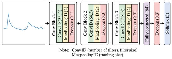
Figure 8.
Architecture of the 1D-CNN model. The network consists of Conv1D layers followed by MaxPooling1D layers. This design enables the model to extract localized temporal features from the 1D Cu2+ concentration data, supporting accurate classification of normal and abnormal states.
Figure 9 illustrates the multimodal CNN architecture used in this study. Two input modalities were derived from each sliding window. The first modality is a 1D residual time series derived from raw Cu2+ values, which is directly fed into a 1D-CNN branch. The second one is a 2D recurrence plot generated from the same window, serving as input to a 2D-CNN branch. Each branch comprises three convolutional blocks, with slightly different numbers of filters that increase with depth in a similar pattern. The feature representations from both branches are then combined through a merge layer and passed to a fully connected layer for classification.
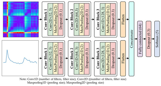
Figure 9.
Architecture of the multimodal CNN model. The network integrates 1D time series and 2D recurrence plot inputs using late fusion with simple concatenation. This design allows the model to simultaneously capture temporal and spatial features, enhancing its ability to classify normal and abnormal Cu2+ concentration states.
For both the 1D-CNN and multimodal CNN models, categorical cross-entropy was used as the loss function, and the Adam (Adaptive Moment Estimation) optimizer was employed with a learning rate of 0.001, a batch size of 64, and a maximum of 50 training epochs. During training, the batch size was selected based on the best performance observed on the validation set, and training was terminated early when no significant improvement in training performance was detected.
Table 1 summarizes the performance metrics (in %) of the evaluated algorithms, with standard deviations shown in parentheses. The results indicate that the multimodal CNN achieves the highest performance, surpassing all other models across every metric and demonstrating the effectiveness of the proposed method in enhancing classification accuracy. Moreover, all CNN-based models show relatively small standard deviations, suggesting greater stability. Among the traditional machine learning approaches, SVM achieves the best results, followed by MLP, RF, and XGB, while decision tree-based models perform comparatively worse. This lower performance may stem from the imbalanced nature of the dataset and the inherent limitation of tree-based methods, which lack translational invariance. In contrast, CNN-based models, including the 1D-CNN, 2D-CNN, and multimodal CNN, consistently demonstrate strong results across all evaluation metrics. Notably, their F1-scores are closely aligned with the corresponding G-measure values, indicating balanced classification across classes. Traditional models, however, display larger discrepancies between these two metrics, reflecting imbalances in classification behavior. Taken together, these findings highlight that CNN architectures not only capture translationally invariant features but also deliver more robust, reliable, and equitable performance compared with conventional machine learning models.

Table 1.
Comparison of classification performance across different models. The multimodal CNN achieves higher accuracy, precision, recall, F1-score, and G-Mean compared with baseline models, demonstrating the advantage of integrating 1D time series and 2D recurrence plot features for reliable detection of abnormal Cu2+ concentration states.
In addition to standard evaluation metrics, it is important to examine each classification model’s performance under both normal and abnormal conditions using a confusion matrix. Figure 10 shows the confusion matrices of various classification models obtained under a specific experimental setting. As illustrated, the confusion matrix reveals that the multimodal CNN not only achieves strong overall performance but also maintains high classification accuracy across all classes. Unlike traditional models, which tend to misclassify rare fault types, the multimodal CNN maintained consistent classification performance, suggesting robustness to real-world imbalance scenarios.
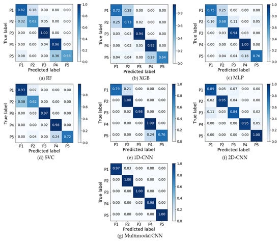
Figure 10.
Confusion matrices of various models. The multimodal CNN achieves higher true positive rates and fewer misclassifications compared with baseline models, demonstrating its superior ability to distinguish between normal and abnormal Cu2+ concentration states. This highlights the benefit of combining temporal and spatial features for reliable process monitoring.
It is important to note that the multimodal CNN demonstrates superior performance on the normal pattern P1, indicating a low false alarm rate. It also performs well on abnormal patterns P2 through P5, reflecting a strong detection capability—an essential attribute for fault detection systems, where early and accurate identification is critical. In addition, the analysis of different data modalities (Figure 10e,f) highlights the strength of the proposed architecture. Comparative results between the 1D-CNN and 2D-CNN indicate that each modality individually captures only partial information. By integrating both modalities, the multimodal CNN effectively leverages complementary features from the raw time series and recurrence plots, leading to enhanced classification performance.
Accurate and early classification of abnormal etchant concentration states is critical in preventing etching defects and reducing production downtime. The proposed multimodal CNN provides a practical solution for real-time process monitoring and can be seamlessly integrated into human-in-the-loop manufacturing systems to support intelligent decision-making. Its high precision and recall reduce the risk of false alarms and missed detections, thereby enhancing trust in automated monitoring systems.
Although the proposed model achieved strong performance, its effectiveness may vary under different process conditions or equipment settings. Since the model was trained on a specific dataset, retraining or fine-tuning may be required when applied to other etching lines or Cu2+ concentration profiles. The current validation is limited to specific PCB etching conditions, and performance could degrade under substantially different scenarios. The approach also assumes representative training data and reliable sensor measurements, and it has not been evaluated with missing or corrupted inputs. Thus, performance outside these conditions remains unverified, and future work will focus on improving the model’s applicability and robustness.
6. Conclusions and Future Work
This study proposed a multimodal convolutional neural network framework for intelligent monitoring of Cu2+ concentration in the PCB etching process. By integrating raw time series data and recurrence plot representations through a sliding window approach, the model effectively captured both temporal dynamics and spatial recurrence patterns associated with normal and abnormal etching conditions. The multimodal architecture enables complementary feature extraction, enhancing classification performance across various process states.
Experimental results demonstrated that the proposed multimodal CNN consistently outperformed conventional machine learning models and single-modality deep learning approaches in terms of accuracy, precision, recall, F1-score, and G-measure. This confirms the effectiveness of multimodal fusion in improving diagnostic sensitivity and robustness, particularly under the imbalanced and noisy conditions typical of industrial monitoring applications.
Despite its strong performance, there are opportunities for further development. Future work will focus on extending the model to support online real-time inference in production environments and integrating adaptive learning mechanisms for continuous model improvement. Additionally, we plan to explore explainable AI techniques, such as SHAP values, to interpret the learned features and improve transparency for industrial users. Expanding the framework to include other critical process variables and employing multivariate multimodal architectures may further enhance its applicability in complex manufacturing systems.
Overall, this work contributes to the advancement of intelligent process monitoring and lays the foundation for more autonomous, resilient, and interpretable quality control systems in the PCB industry.
Author Contributions
Conceptualization, C.-S.C.; Methodology, C.-S.C., P.-W.C. and H.-Y.J.; Software, C.-S.C., P.-W.C., H.-Y.J. and Y.-T.W.; Formal Analysis, C.-S.C., P.-W.C., H.-Y.J. and Y.-T.W.; Investigation, C.-S.C., P.-W.C. and H.-Y.J.; Data Curation, P.-W.C., H.-Y.J. and Y.-T.W.; Writing—Original Draft Preparation, C.-S.C., P.-W.C., H.-Y.J. and Y.-T.W.; Writing—Review and Editing, C.-S.C., P.-W.C., H.-Y.J. and Y.-T.W.; Supervision, C.-S.C. All authors have read and agreed to the published version of the manuscript.
Funding
This research received no external funding.
Data Availability Statement
The original contributions presented in this study are included in the article. Further inquiries can be directed to the corresponding author.
Conflicts of Interest
The authors declare no conflicts of interest.
References
- Fawaz, H.I.; Forestier, G.; Weber, J.; Idoumghar, L.; Muller, P.A. Deep learning for time series classification: A review. Data Min. Knowl. Discov. 2019, 33, 917–963. [Google Scholar] [CrossRef]
- Taherkhani, A.; Cosma, G.; McGinnity, T.M. A deep convolutional neural network for time series classification with intermediate targets. SN Comput. Sci. 2023, 4, 832. [Google Scholar] [CrossRef]
- Wang, W.K.; Chen, I.; Hershkovich, L.; Yang, J.; Shetty, A.; Singh, G.; Jiang, Y.; Kotla, A.; Shang, J.Z.; Yerrabelli, R.; et al. A systematic review of time series classification techniques used in biomedical applications. Sensors 2022, 22, 8016. [Google Scholar] [CrossRef] [PubMed]
- Maden, E.; Karagoz, P. Enhancements for sliding window based stream classification. In Proceedings of the 11th International Joint Conference on Knowledge Discovery, Knowledge Engineering and Knowledge Management (IC3K 2019), Vienna, Austria, 17–19 September 2019. [Google Scholar] [CrossRef]
- Huang, Y.; Zheng, J.; Xu, B.; Li, X.; Liu, Y.; Wang, Z.; Feng, H.; Cao, S. An improved model using convolutional sliding window-attention network for motor imagery EEG classification. Front. Neurosci. 2023, 17, 1204385. [Google Scholar] [CrossRef]
- Chen, W.; Zheng, P.; Bu, Y.; Xu, Y.; Lai, D. Achieving real-time prediction of paroxysmal atrial fibrillation onset by convolutional neural network and sliding window on R-R interval sequences. Bioengineering 2024, 11, 903. [Google Scholar] [CrossRef]
- Falih, B.S.; Sabir, M.K.; Aydın, A. Impact of sliding window overlap ratio on EEG-based ASD diagnosis using brain hemisphere energy and machine learning. Appl. Sci. 2024, 14, 11702. [Google Scholar] [CrossRef]
- Song, W.; Wu, T.; Zhang, Y. A segmented sliding window-based comprehensive periodic feature extraction method for APT classification. In Proceedings of the 2024 IEEE 18th International Conference on Control & Automation (ICCA), Reykjavík, Iceland, 18–21 June 2024. [Google Scholar] [CrossRef]
- Botros, J.; Mourad-Chehade, F.; Laplanche, D. Explainable multimodal data fusion framework for heart failure detection: Integrating CNN and XGBoost. Biomed. Signal Process. Control 2025, 100, 106997. [Google Scholar] [CrossRef]
- Xing, Z.; Ma, G.; Wang, L.; Yang, L.; Guo, X.; Chen, S. Toward visual interaction: Hand segmentation by combining 3-D graph deep learning and laser point cloud for intelligent rehabilitation. IEEE Internet Things J. 2025, 12, 21328–21338. [Google Scholar] [CrossRef]
- Hatami, N.; Gavet, Y.; Debayle, J. Classification of time-series images using deep convolutional neural networks. In Proceedings of the 10th International Conference on Machine Vision (ICMV 2017), Vienne, Austria, 13–15 November 2017. [Google Scholar] [CrossRef]
- Gao, J.; Li, P.; Chen, Z.; Zhang, J. A survey on deep learning for multimodal data fusion. Neural Comput. 2020, 32, 829–864. [Google Scholar] [CrossRef]
- Sleeman, W.C.; Kapoor, R.; Ghosh, P. Multimodal classification: Current landscape, taxonomy and future directions. ACM Comput. Surv. 2022, 55, 1–31. [Google Scholar] [CrossRef]
- Callegari, M.; Carbonari, L.; Costa, D.; Palmieri, G.; Palpacelli, M.C.; Papetti, A.; Scoccia, C. Tools and methods for human robot collaboration: Case studies at i-labs. Machines 2022, 10, 997. [Google Scholar] [CrossRef]
- Mosqueira-Rey, E.; Hernández-Pereira, E.; Alonso-Ríos, D.; Bobes-Bascarán, J.; Fernández-Leal, A. Human-in-the-loop machine learning: A state of the art. Artif. Intell. Rev. 2023, 56, 3005–3054. [Google Scholar] [CrossRef]
- Ranipa, K.; Zhu, W.P.; Swamy, M.N.S. Multimodal CNN fusion architecture with multi-features for heart sound classification. In Proceedings of the 2021 IEEE International Symposium on Circuits and Systems (ISCAS), Daegu, Republic of Korea, 22–28 May 2021. [Google Scholar] [CrossRef]
- Ha, S.; Yun, J.M.; Choi, S. Multimodal convolutional neural networks for activity recognition. In Proceedings of the 2015 IEEE International Conference on Systems, Man, and Cybernetics, Hong Kong, China, 9–12 October 2015. [Google Scholar] [CrossRef]
- Ha, S.; Choi, S. Convolutional neural networks for human activity recognition using multiple accelerometer and gyroscope sensors. In Proceedings of the 2016 International Joint Conference on Neural Networks (IJCNN), Vancouver, BC, Canada, 24–29 July 2016. [Google Scholar] [CrossRef]
- Radu, V.; Tong, C.; Bhattacharya, S.; Lane, N.D.; Mascolo, C.; Marina, M.K.; Kawsar, F. Multimodal deep learning for activity and context recognition. Proc. ACM Interact. Mob. Wearable Ubiquitous Technol. 2018, 1, 1–27. [Google Scholar] [CrossRef]
- Cao, M.; Wan, J.; Gu, X. CLEAR: Multimodal human activity recognition via contrastive learning based feature extraction refinement. Sensors 2025, 25, 896. [Google Scholar] [CrossRef] [PubMed]
- Adarsh, V.; Gangadharan, G.R.; Fiore, U.; Zanetti, P. Multimodal classification of Alzheimer’s disease and mild cognitive impairment using custom MKSCDDL kernel over CNN with transparent decision-making for explainable diagnosis. Sci. Rep. 2024, 14, 1774. [Google Scholar] [CrossRef]
- Alorf, A. Transformer and convolutional neural network: A hybrid model for multimodal data in multiclass classification of Alzheimer’s disease. Mathematics 2025, 13, 1548. [Google Scholar] [CrossRef]
- Chen, J.; Wang, Y.; Zeb, A.; Suzauddola, M.D.; Wen, Y. Multimodal mixing convolutional neural network and transformer for Alzheimer’s disease recognition. Expert Syst. Appl. 2025, 259, 125321. [Google Scholar] [CrossRef]
- Muksimova, S.; Umirzakova, S.; Baltayev, J.; Cho, Y.I. Multi-modal fusion and longitudinal analysis for Alzheimer’s disease classification using deep learning. Diagnostics 2025, 15, 717. [Google Scholar] [CrossRef] [PubMed]
- Khan, M.A.; Ashraf, I.; Alhaisoni, M.; Damaševičius, R.; Scherer, R.; Rehman, A.; Bukhari, S.A.C. Multimodal brain tumor classification using deep learning and robust feature selection: A machine learning application for radiologists. Diagnostics 2020, 10, 565. [Google Scholar] [CrossRef]
- Qu, R.; Xiao, Z. An attentive multi-modal CNN for brain tumor radiogenomic classification. Information 2022, 13, 124. [Google Scholar] [CrossRef]
- Rohini, A.; Praveen, C.; Mathivanan, S.K.; Muthukumaran, V.; Mallik, S.; Alqahani, M.S.; AI-Rasheed, A.; Soufiene, B.O. Multimodal hybrid convolutional neural network based brain tumor grade classification. BMC Bioinform. 2023, 24, 382. [Google Scholar] [CrossRef]
- Jiang, H.; Liu, L.; Lian, C. Multi-modal fusion transformer for multivariate time series classification. In Proceedings of the 14th International Conference on Advanced Computational Intelligence (ICACI), Wuhan, China, 15–17 July 2022. [Google Scholar] [CrossRef]
- Moroto, Y.; Maeda, K.; Togo, R.; Ogawa, T.; Haseyama, M. Multimodal transformer model using time-series data to classify winter road surface conditions. Sensors 2024, 24, 3440. [Google Scholar] [CrossRef]
- Sadras, N.; Pesaran, B.; Shanechi, M.M. Event detection and classification from multimodal time series with application to neural data. J. Neural Eng. 2024, 21, 026049. [Google Scholar] [CrossRef]
- Liu, C.; Wei, Z.; Zhou, L.; Shao, Y. Multidimensional time series classification with multiple attention mechanism. Complex Intell. Syst. 2025, 11, 14. [Google Scholar] [CrossRef]
- Pei, X.; Zuo, K.; Li, Y.; Pang, Z. A review of the application of multi-modal deep learning in medicine: Bibliometrics and future directions. Int. J. Comput. Intell. Syst. 2023, 16, 44. [Google Scholar] [CrossRef]
- El Sakka, M.; Ivanovici, M.; Chaari, L.; Mothe, J. A Review of CNN Applications in smart agriculture using multimodal data. Sensors 2025, 25, 472. [Google Scholar] [CrossRef] [PubMed]
- Bhrad, F.; Abadeh, M.S. An overview of deep learning methods for multimodal medical data mining. Expert Syst. Appl. 2022, 200, 117006. [Google Scholar] [CrossRef]
- Jabeen, S.; Li, X.; Amin, M.S.; Bourahla, O.; Li, S.; Jabbar, A. A review on methods and applications in multimodal deep learning, ACM Trans. Multimed. Comput. Commun. Appl. 2023, 19, 1–41. [Google Scholar] [CrossRef]
- Tang, Q.; Liang, J.; Zhu, F. A comparative review on multi-modal sensors fusion based on deep learning. Signal Process. 2023, 213, 109165. [Google Scholar] [CrossRef]
- Montgomery, D.C. Introduction to Statistical Quality Control, 8th ed.; John Wiley & Sons: Hoboken, NJ, USA, 2020. [Google Scholar]
- Eckmann, J.P.; Kamphorst, O.S.; Ruelle, D. Recurrence plots of dynamical systems. Europhys. Lett. 1987, 4, 973–977. [Google Scholar] [CrossRef]
- Silva, D.F.; de Souza, V.M.A.; Batista, G.E.A.P.A. Time Series Classification Using Compression Distance of Recurrence Plots. In Proceedings of the IEEE 13th International Conference on Data Mining, Dallas, TX, USA, 7–10 December 2013; pp. 687–696. [Google Scholar] [CrossRef]
- Sipers, A.; Borm, P.; Peeters, R. On the unique reconstruction of a signal from its unthresholded recurrence plot. Phys. Lett. A 2011, 375, 2309–2321. [Google Scholar] [CrossRef]
- Iwanski, J.S.; Bradley, E. Recurrence plots of experimental data: To embed or not to embed? Chaos 1998, 8, 861–871. [Google Scholar] [CrossRef]
- Kiranyaz, S.; Avci, O.; Abdeljaber, O.; Ince, T.; Gabbouj, M.; Inman, D.J. 1D convolutional neural networks and applications: A survey. Mech. Syst. Signal Process. 2021, 151, 107398. [Google Scholar] [CrossRef]
- Vaezi Joze, H.R.; Shaban, A.; Iuzzolino, M.L.; Koishida, K. MMTM: Multimodal transfer module for CNN fusion. In Proceedings of the 2020 IEEE/CVF Conference on Computer Vision and Pattern Recognition (CVPR), Seattle, WA, USA, 13–19 June 2020. [Google Scholar] [CrossRef]
- Jaafar, N.; Lachiri, Z. Multimodal fusion methods with deep neural networks and meta-information for aggression detection in surveillance. Expert Syst. Appl. 2023, 211, 118523. [Google Scholar] [CrossRef]
- Cheng, S.; Hou, R.; Li, M. The fusion strategy of multimodal learning in image and text recognition. In Proceedings of the 2024 International Conference on Physics, Photonics, and Optical Engineering (ICPPOE 2024), Singapore, 8–10 November 2024. [Google Scholar] [CrossRef]
- Pereira, L.M.; Salazar, A.; Vergara, L. A comparative analysis of early and late fusion for the multimodal two-class problem. IEEE Access 2023, 11, 84283–84300. [Google Scholar] [CrossRef]
- Pedregosa, F.; Varoquaux, G.; Gramfort, A.; Michel, V.; Thirion, B.; Grisel, O.; Blondel, M.; Prettenhofer, P.; Weiss, R.; Dubourg, V.; et al. Scikit-learn: Machine Learning in Python. J. Mach. Learn. Res. 2011, 12, 2825–2830. [Google Scholar]
- Breiman, L. Random forests. Mach. Learn. 2001, 45, 5–32. [Google Scholar] [CrossRef]
- Chen, T.; Guestrin, F. XGBoost: A scalable tree boosting system. In Proceedings of the 22nd ACM SIGKDD International Conference on Knowledge Discovery and Data Mining, San Francisco, CA, USA, 13–17 August 2016. [Google Scholar]
- Vapnik, V.N. Support-Vector Networks. Mach. Learn. 1995, 20, 273–297. [Google Scholar] [CrossRef]
- Chollet, F. Keras. 2015. Available online: https://github.com/keras-team/keras (accessed on 5 July 2025).
Disclaimer/Publisher’s Note: The statements, opinions and data contained in all publications are solely those of the individual author(s) and contributor(s) and not of MDPI and/or the editor(s). MDPI and/or the editor(s) disclaim responsibility for any injury to people or property resulting from any ideas, methods, instructions or products referred to in the content. |
© 2025 by the authors. Licensee MDPI, Basel, Switzerland. This article is an open access article distributed under the terms and conditions of the Creative Commons Attribution (CC BY) license (https://creativecommons.org/licenses/by/4.0/).