Abstract
The distribution of iron oxide (FeO) across the lunar surface is a key parameter for reconstructing the Moon’s geological evolution and evaluating its in situ resource potential for future exploration. This study applies a spectral-based approach to estimate FeO concentrations using remote sensing reflectance data combined with a Random Forest (RF) regression model. The model was trained on a dataset comprising 89 lunar samples from the Reflectance Experiment Laboratory (RELAB) database, supplemented with compositional data from Apollo samples available via the Lunar Sample Compendium and reflectance spectra from the Clementine mission. Spectral data spanning the visible to shortwave infrared range (415–2780 nm) were analysed, with diagnostic absorption features centred around 950 nm, typically associated with Fe2+. Model validation was conducted against FeO estimates from independent nearside locations not included in the training set, as reported by an external remote sensing study. The trained model was also applied to produce a new global FeO abundance map, demonstrating strong spatial consistency with recent high-resolution reference datasets. These results confirm the model’s predictive accuracy and support the use of legacy multispectral data for large-scale lunar geochemical mapping. This work highlights the potential of combining machine learning techniques, such as Random Forest, with remote sensing data to enhance lunar surface composition analysis, supporting the planning of future exploration and resource utilisation missions.
Keywords:
iron oxide (FeO); lunar regolith; random forest regression; clementine mission; in-situ resource utilization (ISRU) MSC:
62J02; 86A22; 68T30; 68T05; 62H30
1. Introduction
Iron oxide (FeO) is one of the most significant mineralogical components of the lunar regolith, providing valuable insights into the Moon’s magmatic history and its potential for in situ resource utilisation (ISRU) [1,2]. Its distribution across the lunar surface offers a deeper understanding of the composition of lunar basalts and highland materials, with critical implications for both scientific exploration and future lunar mining efforts. Unlike Earth, where iron oxides are typically found in sulphides or hydrated forms, the lunar regolith is dominated by iron in oxide form, owing to the Moon’s distinct magmatic evolution and the absence of water-driven alteration processes [3]. This unique mineralogical composition makes FeO a key target for resource extraction, particularly for oxygen production and other vital resources that may support sustained lunar exploration [4].
The remote sensing of lunar iron and titanium oxides has a long history, beginning with early missions such as that of Charette et al. (1974) [5], which laid the groundwork for modern spectral inversion techniques.
Traditionally, the characterisation of FeO distribution has relied on sample analyses from the Apollo missions, which provide precise geochemical data but are inherently limited in spatial coverage [3,6]. In contrast, remote sensing data from missions like Clementine offer broader spatial coverage, enabling the estimation of FeO concentrations across extensive lunar regions [1,2]. Clementine’s imaging capabilities, however, vary in spatial resolution—ranging from 100–200 m per pixel in some areas to lower resolutions elsewhere [7,8]. This means that each pixel represents an area much larger than individual Apollo sampling sites, making direct comparisons between remote sensing and sample-based analyses challenging. Over the past four decades, substantial progress has been made in mapping the global distribution of lunar FeO using Clementine multispectral data and traditional empirical regression techniques [2,9,10]. These methods established the first high-resolution elemental maps of the lunar surface and remain a cornerstone of lunar geochemical analysis. Nevertheless, such approaches typically rely on fixed polynomial relationships between reflectance ratios and FeO abundance, which may not fully capture the non-linear spectral–geochemical interactions observed across diverse lunar terrains.
This study addresses these limitations by applying advanced statistical learning algorithms—specifically Random Forest (RF) regression models—to estimate FeO concentrations across the lunar surface. We train these models using a comprehensive dataset that integrates spectral reflectance data from the Reflectance Experiment Laboratory (RELAB) database [11], geochemical data from Apollo lunar samples via the Lunar Sample Compendium [12], and orbital spectral data from the Clementine mission [13]. The resulting model was validated against independent FeO estimates from a separate remote sensing study that focused on diverse nearside environments, including Catharina and Cyrillus craters [14], providing a robust assessment of the model’s reliability and generalisation across varied geological settings. This confirmed the model’s strong predictive performance in estimating FeO concentrations with accuracy. The work contributes to the development of improved models for lunar exploration and ISRU strategies by offering a highly accurate and validated approach to FeO distribution mapping. The application of machine learning to lunar geochemistry is an emerging field [15,16], and this study demonstrates its potential to refine our understanding of lunar resources, directly supporting future efforts to utilise these materials in situ as part of a broader strategy for sustainable exploration.
Recent advances in machine learning (ML) have demonstrated the potential of algorithms such as Support Vector Machines (SVMs) and Convolutional Neural Networks (CNNs) for planetary mineralogical mapping [9,10,17,18,19]. While these approaches have achieved promising results, many rely on highly complex models trained on very limited ground-truth datasets—sometimes fewer than 40 samples. This can limit robustness and generalisation to broader lunar terrains. Preliminary tests with SVMs in this study showed that their performance was highly sensitive to kernel choice and regularisation parameters, resulting in unstable predictions. In contrast, Random Forest regression offers inherent robustness against overfitting, stable performance on small- to medium-sized datasets, and improved interpretability through feature importance analysis.
Moreover, comprehensive cross-mission evaluations—particularly between Clementine multispectral data and hyperspectral data from Chandrayaan-1 M3—remain limited, and large-scale assessments across geologically diverse terrains have not been widely reported. To address this, we developed a Random Forest regression model specifically tailored to Clementine UVVIS+NIR data, generating a new global FeO map. The model was quantitatively validated against a state-of-the-art high-resolution FeO dataset and evaluated regionally across both basaltic maria and feldspathic highlands, providing a robust and interpretable methodology for near-global FeO mapping that enhances cross-mission comparability and supports future exploration and ISRU planning.
The specific objectives of this study are as follows:
- To develop a Random Forest regression model for predicting lunar FeO abundance using multispectral Clementine UVVIS+NIR data.
- To generate a new global FeO abundance map by applying the trained model to harmonised Clementine mosaics, offering near-global coverage of the lunar surface.
- To evaluate the model’s predictive performance through quantitative comparisons with ground-truth measurements, established empirical models [14], and one of the most recent high-resolution FeO datasets [20].
- To assess the model’s applicability for large-scale lunar resource assessment and in situ resource utilisation (ISRU) planning.
2. Materials and Methods
2.1. Data Acquisition
2.1.1. Lunar Sample Data from Apollo Missions
We utilised 89 lunar samples from the Lunar Sample Compendium, selected for their availability of both geochemical data and corresponding reflectance spectra in the Reflectance Experiment Laboratory (RELAB) database. The FeO concentration (), expressed in weight percent (wt.%), was determined by X-ray fluorescence (XRF) spectroscopy under controlled laboratory conditions.
where is the XRF signal intensity attributed to FeO, and is the total signal intensity from all detectable elements.
2.1.2. Clementine Mission Data
Clementine multispectral data (11 bands spanning 415–2780 nm) with variable spatial resolution (up to 100–200 m/pixel) served dual purposes.
- Defining the 11 central wavelengths used to extract discrete reflectance values from RELAB spectra.
- Providing input reflectance data for spatial FeO prediction and independent validation.
Radiometrically and photometrically corrected data were obtained from the Planetary Data System (PDS). Spectral reflectance () was calculated as
where is the observed intensity at wavelength , and is the intensity from a reference surface (e.g., onboard calibration target) [2].
2.1.3. Laboratory Reflectance Spectra from RELAB
The 89 Apollo sample spectra (300–2780 nm) were obtained from the Reflectance Experiment Laboratory (RELAB) database, measured under standard viewing geometry (incidence angle , emission angle ). These high-quality laboratory measurements were used directly without additional noise filtering or photometric corrections. To ensure compatibility with Clementine’s 11-band configuration, the continuous RELAB spectra were resampled to match the mission’s central wavelengths (415, 750, 950 nm, etc.) using Gaussian interpolation.
where are Clementine’s band centres and their effective bandwidths. This preserved the diagnostic Fe2+ absorptions near 950 and 1050 nm [2] while ensuring consistency across datasets.
2.2. Data Integration for FeO Mapping
The reflectance vectors derived from RELAB spectra, sampled at the eleven Clementine wavelengths, were paired with FeO concentrations measured in Apollo and Luna samples to construct the training dataset. This structured input enabled the Random Forest (RF) model to learn the nonlinear relationship between spectral features and FeO content, leveraging RF’s proven efficacy in handling high-dimensional remote sensing data with limited training samples [21].
The model was trained using absolute reflectance values at the eleven Clementine wavelengths. No derived spectral parameters (e.g., band ratios or continuum-removed features) were used. To examine possible albedo effects, we analysed the correlation between reflectance at 750 nm—a proxy for brightness—and the model residuals. No significant dependency was observed, indicating that prediction errors are not dominated by albedo variations but rather reflect genuine compositional differences.
Only those samples with both RELAB spectra and chemical analysis were included in the training set. The validation strategy, including additional Apollo and Luna sites lacking RELAB spectra, is described in Section 2.5.
2.3. Statistical Learning Approach for FeO Prediction
2.3.1. Random Forest Regression
Let
where are feature vectors and their responses. These pairs are assumed to be independent and identically distributed (i.i.d.) draws from an unknown joint distribution [22,23]. The aim is to estimate the regression function
Random Forest (RF) is a nonparametric ensemble learning method that builds upon decision trees to estimate . Each individual tree is constructed using a bootstrap sample of the training data and incorporates random feature selection at each split, represented by the random parameter [22,24]. Recent benchmarks suggest that RF retains superior performance compared to deep learning alternatives in small-sample regimes, as often encountered in planetary science datasets [25]. A regression tree partitions the input space into disjoint regions and predicts using the average response in each region:
A Random Forest predictor is obtained by averaging B such randomised trees.
where each is a bootstrap sample of the training data and captures the randomness used to construct the b-th tree. This averaging procedure reduces variance and mitigates overfitting, which is particularly important when working with small datasets [26].
The prediction error of RF can be decomposed into bias and variance:
Letting and for , the variance of the RF estimator becomes
Under suitable regularity conditions (e.g., subsampling rate, increasing tree depth), Random Forests have been proven to be consistent estimators of [23,27].
Beyond its theoretical foundations, Random Forest has demonstrated robust empirical performance in modelling non-linear relationships within high-dimensional spectral datasets [22]. In our application to lunar FeO estimation, the RF model was trained on the Apollo dataset () using 11 spectral reflectance bands . The RF prediction takes the form
where is the prediction of the i-th tree.
Two domain-specific modifications were introduced to enhance model performance.
- Feature importance weighting: Spectral bands near 950 nm and 1050 nm, associated with Fe2+ absorptions [2], were prioritised during node splitting, following interpretability frameworks validated in recent toxicological studies [28].
- Asymmetric error handling: The loss function imposed a greater penalty on overestimations than on underestimations, reflecting the greater cost of false positives in resource exploitation planning.
Furthermore, recent studies have drawn connections between Random Forests and kernel methods, offering an alternative functional interpretation of the algorithm [23]. Overall, Random Forest provides a powerful, interpretable, and robust approach to regression in remote sensing contexts, particularly when dataset size constraints preclude the use of more complex architectures [25,26].
2.3.2. Model Training Protocol
The training process incorporated both spectral and geochemical constraints.
- Data partitioning: The 89 samples were split into training datasets () and validation datasets (), preserving the original distribution of FeO concentrations (range: 0.5–22 wt.%) across both sets.
- Error metric selection: The Huber Loss [29] was minimised during training as it balances sensitivity to outliers (prevalent in heterogeneous lunar samples) with robustness to small-scale spectral variations.where was empirically optimised for lunar FeO predictions.
- Geochemical sanity checks: Predicted FeO values exceeding the maximum Apollo sample concentration (22 wt.%) were physically constrained via post-processing.
2.3.3. Model Configuration
The model was implemented in Python (version 3.12.2) using the scikit-learn library (sklearn.ensemble. RandomForestRegressor), a widely used toolkit for machine learning across scientific and industrial domains. The Random Forest hyperparameters were optimised through an exhaustive grid search aimed at minimising the validation error. The final configuration achieved a balance between model complexity, computational efficiency, and generalisation performance. It is detailed below:
- n_estimators = 100: Number of decision trees in the forest. Increasing this value typically improves prediction stability, although at the cost of greater computational demand.
- max_depth = None: Allows trees to grow without limit until all leaves are pure or contain fewer than the minimum number of samples for a split. This flexibility enables the model to capture complex and non-linear relationships in the spectral data.
- min_samples_split = 2: The minimum number of samples required to split an internal node. A low value allows the model to create finely partitioned decision regions, which is particularly useful when dealing with small datasets or subtle spectral differences.
- min_samples_leaf = 1: Minimum number of samples required to form a leaf node. Setting this to 1 helps preserve local spectral variability by allowing the model to capture detailed trends that may appear in individual observations.
This configuration allows the Random Forest model to remain sensitive to subtle reflectance variations associated with FeO content, particularly in heterogeneous lunar samples. At the same time, ensemble averaging across the 100 trees effectively reduces overfitting, thereby enhancing the robustness of the predictions.
Regression ensemble methods such as Random Forest have shown strong performance in modeling non-linear relationships in other scientific domains. For example, more flexible ensemble approaches, such as Multivariate Adaptive Regression Splines (MARS), have been applied successfully to energy systems [30], suggesting their promising utility for geochemical inference and planetary remote sensing tasks.
2.4. Preliminary Evaluation of Alternative Machine Learning Models
Preliminary experiments were conducted to explore alternative machine learning algorithms for FeO prediction, including Support Vector Machines (SVMs) with different kernel functions (linear, polynomial, radial basis function, and sigmoid). These tests aimed to assess whether more complex models could outperform Random Forest regression given the available dataset.
The results, summarised in Table 1, show that the SVM models consistently underperformed relative to Random Forest. Non-linear kernels (polynomial, RBF) exhibited high sensitivity to hyperparameter settings and tended to overfit, leading to unstable predictions and reduced generalisation performance. The linear kernel underfit the data, leading to reduced accuracy. In contrast, Random Forest demonstrated robust predictive performance, stable error metrics, and interpretability through feature importance analysis. Consequently, Random Forest was selected as the primary regression method for the study.

Table 1.
Preliminary performance comparison between Random Forest and Support Vector Machines (SVMs) with different kernels. Metrics are based on cross-validation results.
2.5. Validation Using External Lunar Data (M3 from Chandrayaan-1)
To externally validate the model, reflectance data from the Moon Mineralogy Mapper (M3) aboard the Chandrayaan-1 mission were employed [31]. The validation focused on surface locations corresponding to Apollo and Soviet Luna landing sites for which reliable FeO ground-truth abundances are available. These particular landing site samples were excluded from the training dataset due to the lack of laboratory reflectance spectra in the RELAB spectral library, even though their FeO abundances are well-characterised and their locations are covered by M3.
Following the same methodology applied to Clementine data, reflectance values were extracted at the eleven central wavelengths employed as input features for the Random Forest model. These values were obtained at the precise geographic coordinates of the selected landing sites, allowing for direct comparison between model predictions and ground-truth FeO concentrations.
The performance of the model was also benchmarked against the approach proposed by Kumar (2023) [14], who applied several regression-based inversion models—linear, polynomial, logarithmic, exponential, and power functions—using M3 data to estimate FeO content. Their methodology, grounded in physically-based modeling and empirical optimisation, provides a valuable point of comparison as it constitutes a well-established, non-machine-learning alternative.
Importantly, the validation not only evaluated consistency with known reference values but also tested the model’s robustness across different remote sensing instruments and data sources. While the model developed in this study was trained using Clementine reflectance spectra, the benchmarking against M3-based models enabled a cross-instrument evaluation of its generalisation capability.
This dual-validation strategy—against both ground-truth data and an independently published model—provided a comprehensive framework to assess the reliability and operational applicability of the Random Forest model under realistic lunar exploration conditions.
2.6. Data Limitations and Mitigation Strategies
Three key limitations in the training dataset were identified and addressed.
- Spatial bias in Apollo samples: The 89 lunar samples used for training originate exclusively from the Moon’s nearside (primarily Mare Imbrium and highland regions [3]), introducing potential biases when predicting FeO concentrations in unsampled terrains such as farside basalts or polar regions. To mitigate this limitation, we prioritised validation sites located in geologically distinct environments (e.g., the Catharina Crater highlands). Moreover, the spectral complexity observed in other lunar regions—such as the Chang’e-3 landing site—further underscores the importance of validating predictive models across geologically heterogeneous terrains [32].
- Resolution mismatch: Clementine’s spectral resolution (100–200 m/pixel) averages FeO signatures over areas ~104–105× larger than Apollo sample spots. While this limits direct pixel-to-sample comparisons, we
- Excluded mixed-pixel regions (e.g., crater edges) from validation using LROC NAC images [33].
- Selected homogeneous geological units around each Apollo landing site to reduce the impact of subpixel heterogeneity.
- Space weathering effects: Laboratory spectra (RELAB) lack space weathering dynamics (e.g., solar wind irradiation), which alter spectral slopes [34]. We accounted for this by
- Weighting M3 validation data by optical maturity (OMAT index [2]).
- Excluding fresh ejecta () from model training.
While these strategies mitigate systematic uncertainties in global FeO predictions, they do not eliminate them entirely.
Irreducible dataset constraints: The 89 Apollo samples with paired FeO measurements and RELAB spectra represent the only globally available dataset of their kind as of 2025. This limitation is intrinsic to lunar exploration: no additional samples with comparable geochemical–spectral pairing exist, and future missions (e.g., Artemis) will require years to generate equivalent ground-truth data [35]. To ensure robustness despite this constraint,
- The model was validated exclusively on independent orbital data (Clementine and M3) from regions outside Apollo sampling sites (e.g., Catharina Crater).
- Feature selection prioritised spectral bands with known physical links to FeO (950 nm, 1050 nm) over purely statistical correlations [2].
While the preceding sections describe the datasets and preprocessing steps, it is also important to explicitly discuss the methodological limitations of previous lunar FeO mapping approaches and how the present study addresses them.
Previous approaches to lunar FeO mapping have faced several methodological constraints that limit their robustness and applicability. Empirical regression models were typically calibrated using small, spatially localised ground-truth datasets, making it difficult to generalise predictions across geologically diverse terrains. More advanced machine learning algorithms, such as Support Vector Machines and Convolutional Neural Networks, have been explored in recent studies, but these methods typically require large training datasets to achieve stable performance and avoid overfitting. In practice, the limited number of FeO reference samples available for the Moon has led to highly variable predictions and reduced reliability. Furthermore, few studies have attempted modern cross-mission validation, and a globally consistent FeO map derived from Clementine multispectral data has not previously been produced.
The Random Forest regression approach adopted here is specifically designed to overcome these limitations. By aggregating multiple decision trees, Random Forest mitigates overfitting and performs well even with relatively small training datasets. Its ensemble nature enables robust generalisation across different geological terrains while maintaining interpretability through feature importance analysis. This methodological choice, combined with the near-global coverage of Clementine UVVIS+NIR observations, enables the generation of a new, validated global FeO abundance map that can be quantitatively compared with state-of-the-art high-resolution products from other missions.
3. Results and Validation
This section presents a comprehensive evaluation of the proposed Random Forest (RF) model for lunar FeO content prediction, in direct comparison with empirical models proposed by Kumar (2023) [14]. The analysis integrates overall performance metrics, site-specific accuracies, error distribution characteristics, and insights into the RF model’s internal feature importance.
Table 2 summarises the key performance metrics for each model: Mean Absolute Error (MAE), Root Mean Square Error (RMSE), and the Coefficient of Determination (R2). These metrics quantify the overall accuracy and goodness of fit of each model on the validation dataset.
Table 2.
Comparative performance metrics of FeO prediction models.
As shown in Table 2, the polynomial and linear empirical models derived by Kumar et al. (2024) [14] demonstrate the highest overall accuracy on this validation set, with Kumar—Poly achieving the best MAE (0.9009), RMSE (1.0988), and R2 (0.9344). While competitive with an R2 of 0.8996, our Fernandez—RF model exhibits slightly higher error metrics (MAE of 1.0823, RMSE of 1.3596) compared to Kumar’s top-performing models. The exponential model proposed by Kumar shows the weakest performance among all evaluated models.
To provide a comprehensive overview of the models’ performance at individual sites, Table 3 presents the actual FeO content, along with the predicted values and corresponding absolute errors for all evaluated models (Kumar’s empirical models and Fernandez—RF). This detailed breakdown enables direct comparison of each model’s accuracy across various lunar landing sites.
Table 3.
Comparative site-specific predictions and absolute errors for all models.
The performance of the models was further analyzed across different ranges of actual FeO concentration to assess consistency in predictive accuracy. Table 4 presents the MAE, RMSE, and R2 for the Fernandez—RF model and the Kumar—Poly model (as the best-performing empirical model) within three distinct FeO concentration bins: low (FeO < 8 wt.%), medium (8 ≤ FeO ≤ 14 wt.%), and high (FeO > 14 wt.%).
Table 4.
Performance metrics by FeO concentration bins (wt.%).
Results in Table 4 indicate varying performance across FeO ranges. The Kumar—Poly model generally shows better accuracy in the low and high FeO concentration bins. However, our Fernandez—RF model demonstrates superior performance in the medium FeO range (8 ≤ FeO ≤ 14 wt.%), suggesting robust capability in predicting FeO values within this critical intermediate range.
Figure 1 illustrates the overall agreement between the actual FeO content and the predictions generated by our Fernandez—RF model. This parity plot illustrates the model’s accuracy, predictive linearity, and potential systematic biases or outliers across the range of FeO values. Ideally, points would cluster along the 1:1 line.
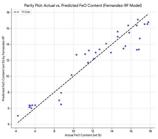
Figure 1.
Parity plot of actual FeO content versus predicted FeO content by the Fernandez—RF model on the validation dataset. The diagonal dashed line represents perfect agreement (1:1 line).
Further insight into the model performance is provided by Figure 2, which displays the distribution of residuals (actual—predicted values) for the Fernandez—RF model and for Kumar’s best performing model (Kumar—Poly). Analyzing the spread and symmetry of residuals indicates the reliability and consistency of the predictions, highlighting tendencies toward over- or underestimation.
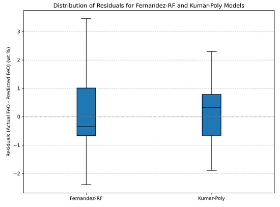
Figure 2.
Box plots of residuals (actual FeO—predicted FeO) for the Fernandez—RF model and Kumar—Poly model. The plots illustrate the spread and central tendency of prediction errors for each model.
The distribution of residuals was further examined through a plot of residuals versus predicted values for the Fernandez—RF model (Figure 3). This diagnostic plot helps identify patterns in the errors across the prediction range, such as heteroscedasticity or systematic biases that might not be evident from overall metrics alone. Ideally, residuals should be randomly scattered around zero, indicating a well-fitted model.
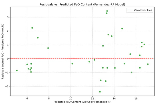
Figure 3.
Residuals (actual FeO—predicted FeO) versus predicted FeO content for the Fernandez—RF model. This plot helps identify patterns in the error distribution across the range of predictions.
Finally, to understand the internal mechanisms of the Fernandez—RF model, Figure 4 illustrates the relative importance of each of the 11 Clementine-equivalent spectral wavelengths used as input features. This provides insight into which wavelengths contribute most significantly to the model’s FeO predictions.
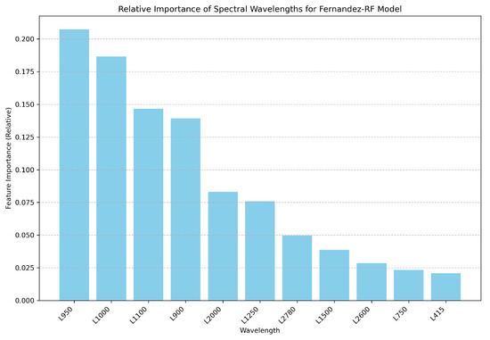
Figure 4.
Relative importance of the input spectral wavelengths used by the Fernandez—RF model. The wavelengths are L950 (0.207), L1000 (0.187), L1100 (0.147), L900 (0.139), L2000 (0.083), L1250 (0.076), L2780 (0.050), L1500 (0.039), L2600 (0.029), L750 (0.023), L415 (0.021).
3.1. Global FeO Map and Comparison with State-of-the-Art Datasets
A global map of FeO abundance was generated by applying the trained Random Forest (RF) regression model to a harmonised multispectral mosaic of the lunar surface. The input dataset was created by combining the Moon Clementine UVVIS 5-Band Warped Image Mosaic. Ref. [36] , radiometrically and geometrically controlled and photometrically normalised, with the Moon Clementine NIR Standard Calibration Mosaic (ISIS format, 50 m/pixel resolution). The UVVIS mosaic (200 m/pixel resolution; five bands: 415, 750, 900, 950, and 1000 nm) was reprojected and co-registered with the NIR mosaic to produce a unified global image containing eleven spectral bands. The resulting dataset covers latitudes from 70° S to 70° N and longitudes from −180° to +180° at 500 m/pixel spatial resolution, enabling pixel-by-pixel prediction of FeO content across the lunar nearside and farside.
The RF-predicted FeO abundance map (Figure 5) captures the large-scale compositional variations in the lunar surface, including the high FeO concentrations characteristic of mare basalts and the low FeO content of the highlands. To quantitatively assess its consistency with contemporary reference products, the predictions were compared with the global FeO map recently published by Zhang et al. (2023) [20] (see Figure 6) . This reference dataset was constructed by fusing Chang’E-5 geochemical analyses with KAGUYA Multiband Imager (MI) observations at 59 m/pixel resolution, providing one of the most detailed FeO distributions currently available. Both maps were projected onto a common equirectangular grid prior to comparison, accounting for differences in native spatial resolution and map projection.
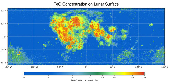
Figure 5.
Global FeO abundance map predicted by Random Forest (RF), showing mare–highland contrasts (0–20 wt.% FeO).
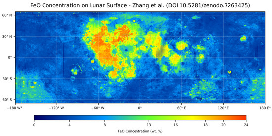
Figure 6.
Global FeO abundance map (wt.%) generated from the data provided by Zhang et al. [20] and shared on Zenodo (DOI: https://doi.org/10.5281/zenodo.7263425), derived from Chang’E-5 samples and KAGUYA MI data at 59 m/pixel resolution. Color scale indicates FeO concentrations ranging from 0–25 wt.%.
The comparison shows a strong overall agreement between the RF predictions and the Zhang et al. dataset. Pixel-wise statistical analysis yielded a Root Mean Square Error (RMSE) of 1.97 wt.%, a Coefficient of Determination (R2) of 0.83, and a mean bias of 0.06 wt.%. Visual inspection of the two maps further reveals consistent spatial patterns of FeO enrichment and depletion across major lunar geological units. Residual discrepancies may partially reflect persistent artifacts from the original high-resolution KAGUYA MI mosaic [37], with minor additional effects introduced during reprojection and resampling procedures.
3.2. Local Geological Comparisons
The predictive performance of the Random Forest (RF) model was further assessed across several geologically diverse lunar regions. The analysis included four basaltic maria (Mare Crisium, Mare Serenitatis, Oceanus Procellarum, and Mare Nectaris), two highland mountain ranges (Montes Taurus and Montes Haemus), and a valley region (Taurus–Littrow), encompassing a broad range of lunar geological terrains.
Quantitative comparison metrics (RMSE, , and mean bias) for all seven regions are reported in (Table 5). The results demonstrate that the RF-based FeO abundance estimates are consistently close to the reference dataset by Zhang et al. (2023) [20], with RMSE values typically around 1–2 wt.% and values above 0.80 in all areas.
Table 5.
Model validation statistics by region.
For visual inspection, three representative regions were selected for detailed analysis (Figure 7, Figure 8 and Figure 9). These regions—Mare Serenitatis (a basaltic mare), Oceanus Procellarum (a geologically and compositionally more complex mare), and Montes Haemus (a feldspathic highland terrain)—were chosen to demonstrate the model’s performance across diverse geological settings.
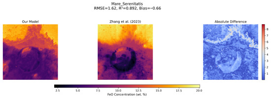
Figure 7.
Comparison of FeO abundance maps for the Mare Serenitatis region, a basaltic mare. The figure shows the RF-predicted FeO abundance (left), the high-resolution Zhang et al. (2023) [20] map (middle) , and the absolute difference (right).
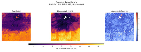
Figure 8.
Comparison of FeO abundance maps for the Oceanus Procellarum region, a vast and compositionally complex mare. The RF-predicted FeO abundance (left), the Zhang et al. (2023) [20] map (middle), and the absolute difference (right).
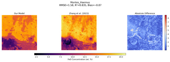
Figure 9.
Comparison of FeO abundance maps for the Montes Haemus region, a representative feldspathic highland terrain. The RF-predicted FeO abundance (left), the Zhang et al. (2023) [20] map (middle), and the absolute difference (right).
For each selected region, the Random Forest (RF) predicted FeO abundance (left panel), the high-resolution FeO map (middle panel) [20], and the absolute difference between the two datasets (right panel) are presented.
In all three examples, the RF predictions capture both large-scale compositional patterns and the finer geological structures observed in the high-resolution Zhang et al. dataset. Strong agreement with the reference dataset is shown in the mare basins (Mare Serenitatis: RMSE = 1.62 wt.%, = 0.89, Bias = −0.66; Oceanus Procellarum: RMSE = 1.95 wt.%, = 0.84, Bias = −0.63). Even in challenging highland regions such as Montes Haemus, where spectral mixing and topographic effects are more pronounced, the RF model maintains robust predictive accuracy (RMSE = 1.58 wt.%, = 0.84), illustrating its reliability in low-FeO regions.
4. Discussion
The analysis demonstrates that a Random Forest (RF) regression model can accurately predict FeO abundance from multispectral Clementine data with high spatial coverage. In addition to validation against models based on Moon Mineralogy Mapper (M3) data [14], a global FeO abundance map was generated by applying the RF model to harmonised Clementine UVVIS and NIR mosaics. This approach illustrates the capability of statistical learning techniques to exploit multispectral datasets of moderate spectral resolution for large-scale lunar geochemical mapping.
The RF-predicted global FeO map (Figure 5) shows strong consistency with one of the most recent and advanced FeO datasets, published by Zhang et al. (2023) [20] which integrates Chang’E-5 geochemical analyses with KAGUYA Multiband Imager (MI) observations (Figure 6). A pixel-by-pixel comparison yielded a Root Mean Square Error (RMSE) of 1.97 wt.%, a Coefficient of Determination () of 0.83, and a negligible mean bias of 0.06 wt.%. Visual comparison confirms that both datasets capture similar FeO enrichment patterns in basaltic maria and depletion in feldspathic highlands. Residual differences can be partly attributed to noise introduced during the processing of high-resolution KAGUYA MI mosaics (Ohtake et al., 2008) [37], as well as to reprojection artefacts introduced during resampling. These findings indicate that the RF model achieves an accuracy comparable to modern high-resolution reference products while relying solely on Clementine multispectral observations.
Regional analyses conducted across geologically diverse terrains (Table 5) indicate that the RF model generalises effectively across various lunar environments. Basaltic mare basins, such as Mare Crisium (RMSE = 0.96 wt.%, = 0.87) and Mare Nectaris (RMSE = 1.13 wt.%, = 0.85), were reproduced with high fidelity. Even in highland regions such as Montes Haemus (RMSE = 1.58 wt.%, = 0.84), and in rugged terrains like the Taurus–Littrow Valley, where spectral mixing and topographic effects are more pronounced, the model maintained reliable predictive performance. Figure 7, Figure 8 and Figure 9 illustrate examples of these regional comparisons, highlighting how the RF approach preserves spatial accuracy across both maria and highlands, from regional to global scales.
Table 2 shows that the polynomial regression model by Kumar et al. (2024) achieves the lowest MAE and RMSE, along with the highest , confirming its robust predictive capability for FeO. The Random Forest model yields a competitive of 0.8996, albeit with slightly higher overall error metrics. However, a detailed site-specific examination (Table 3) reveals variable accuracies across lunar landing sites, underscoring the importance of evaluating models beyond aggregated metrics. For instance, at Luna16, the RF model’s prediction (17.09 wt.%) is closer to the actual value (16.7 wt.%) than that of Kumar—Poly’s (16.14 wt.%) despite the latter’s higher overall . Conversely, at AP17LRV6, Kumar—Poly (8.90 wt.%) is considerably closer to the actual value (10.3 wt.%) than RF (12.69 wt.%), highlighting localised strengths and weaknesses. These discrepancies highlight the complex nature of spectral signatures and the varying sensitivity of different models to specific geochemical contexts. Bin-wise performance analysis (Table 4) further reveals that the RF model provides enhanced accuracy in the intermediate FeO concentration range (8 ≤ FeO ≤ 14 wt.%), which is particularly valuable for identifying regions with moderate FeO content that may serve as optimal targets for ISRU applications.
Visual diagnostics further corroborate these quantitative findings. The parity plot (Figure 1) for the RF model displays a clear clustering of predicted values along the 1:1 line, indicating a good overall fit despite minor scatter consistent with the reported error metrics. The residual distributions (Figure 2) indicate that, although the RF model exhibits slightly wider residual spread compared to Kumar’s polynomial model, both models maintain a central tendency near zero, suggesting the absence of pronounced systematic bias. Additionally, the residuals-versus-predicted plot (Figure 3) confirms a largely random distribution of errors around zero, with no evidence of notable heteroscedasticity or systematic trends that could compromise the model’s general applicability.
Furthermore, the feature-importance analysis (Figure 4) offers valuable insights into the model’s dependence on specific Clementine wavelengths, particularly L950, L1000, L1100, and L900. These bands are known to be sensitive to ferrous-iron absorption features, confirming the physical basis of the Random Forest model’s predictive capacity and its ability to capture meaningful geochemical relationships from a limited set of spectral inputs. This observationaligns with earlier studies on ferrous-iron spectral features in lunar materials [5]. Future improvements in interpretability could be achieved by applying SHAP analysis [38], which would quantify the marginal contribution of each spectral feature to individual predictions.
Regarding dataset characteristics, the Clementine UVVIS+NIR mission provided near-global coverage of the lunar surface, albeit with only 11 discrete spectral bands (5 in UVVIS: 415, 750, 900, 950, and 1000 nm and 6 in NIR: 1100, 1250, 1500, 2000, 2600, and 2780 nm) [2], at spatial resolutions of approximately 100–500 m per pixel. This relatively sparse spectral sampling, although seemingly a limitation, is effectively mitigated by the Random Forest algorithm’s capacity to model complex, non-linear relationships. Consequently, competitive predictive performance is achieved with fewer input variables, maximising the utility of Clementine’s unique near-global spatial coverage. By contrast, empirical models based on Moon Mineralogy Mapper (M3) data [31] provide higher spectral resolution (86 contiguous bands) and finer spatial detail (70–140 m per pixel) but lack complete global coverage.
The choice of Random Forest over other machine learning techniques is further supported by its capacity to deliver accuracy comparable to modern high-resolution approaches [20] while maintaining robustness against overfitting in a data-limited context. Unlike deep neural networks, which require extensive training data and computational resources, Random Forest performs effectively with the limited number of lunar ground-truth FeO measurements available. This balance between model complexity and generalisation capability is particularly advantageous for planetary datasets characterised by sparse in situ sampling and legacy multispectral observations.
An intrinsic limitation of the Clementine dataset is its inability to differentiate between different oxidation states of iron (Fe2+ vs. Fe3+), as its spectral bands (415–1000 nm) lack the spectral resolution needed to isolate diagnostic Fe2O3 absorption features at 530 nm and 860 nm [39]. This limitation constrains the model’s ability to account for oxidised iron phases, such as hematite, which have been detected at high lunar latitudes [39]. Nevertheless, more than 90% of lunar iron occurs as FeO under reducing conditions [3], and Clementine’s band centres (e.g., 750/950 nm) preferentially detect Fe2+ in silicates [2]. Future research could incorporate hyperspectral datasets (e.g., M3’s 86 narrow bands) to resolve Fe3+ absorption signatures at 530 and 860 nm, thereby enhancing oxidation state mapping [31].
The application of statistical learning techniques to lunar mineralogical mapping is well established and has been successfully demonstrated across multiple datasets. Similar approaches have been successfully applied to Chang’e mission data [40,41] and M3 observations, as in the study by Zhang et al. (2023) [20], which estimated FeO and TiO2 abundances. Neural network-based models, such as back-propagation neural networks (BPNNs), have also been employed to derive FeO and TiO2 distributions from Chang’e data [40], further illustrating the versatility of machine learning approaches in lunar geochemistry. Additionally, global mineral distribution maps derived from Chang’e-1 observations have demonstrated the feasibility of learning-based techniques for extrapolating FeO estimates across geologically diverse regions [10].
Overall, these findings highlight the capability of Random Forest regression to efficiently capture complex spectral relationships and to produce accurate, spatially consistent mineralogical maps of the Moon. By leveraging legacy multispectral datasets such as Clementine, the model achieves accuracy comparable to hyperspectral methods while enabling comprehensive planetary coverage. This offers a validated methodology for lunar FeO mapping, with implications not only for scientific investigation but also for future in-situ resource utilisation (ISRU) planning. In particular, regions with intermediate FeO concentrations (8–14 wt.%) identified by the model may serve as promising candidates for oxygen extraction via the reduction of ilmenite (FeTiO3), a well-established ISRU pathway [42,43]. Similarly, FeO-rich basalts are of interest for sintering-based construction as well as for metal extraction processes [44]. Thus, the generated FeO maps contribute to the preliminary identification and prioritisation of potential ISRU sites across the lunar surface.
5. Conclusions
This study has developed and evaluated a Random Forest (RF) regression model for predicting lunar FeO concentrations from Clementine UVVIS+NIR spectral data. The model was benchmarked against established empirical approaches based on Chandrayaan-1 Moon Mineralogy Mapper (M3) data [14], showing competitive predictive accuracy with an overall R2 of 0.8996 and particular strength in the medium FeO concentration range (8–14 wt.%).
Applying the trained model to harmonised Clementine mosaics, a new global FeO abundance map was generated. Comparison with one of the most recent and advanced FeO datasets [20], which combines Chang’E-5 geochemical analyses with KAGUYA Multiband Imager observations, showed strong agreement (RMSE = 1.97 wt.%, = 0.83, negligible mean bias). This validates the capability of the RF approach to produce spatially consistent, high-fidelity geochemical maps from legacy multispectral datasets. Regional analyses further confirmed that the model generalises effectively across geologically diverse environments, reproducing FeO distributions in both basaltic maria and feldspathic highlands with high fidelity.
The use of Clementine data, providing near-global spatial coverage (100–500 m/pixel), offers distinct advantages for large-scale lunar exploration and in situ resource utilisation (ISRU) planning. The resulting global FeO map is uniquely suited for the following:
- Comprehensive Resource Assessment: Identifying promising ISRU regions across the entire lunar surface, free from the spatial constraints of targeted missions.
- Strategic Mission Planning: Supporting the selection of landing sites and operational regions for long-term exploration and resource extraction activities.
- Complementary Mapping: Providing a broad, planetary-scale context that complements higher-resolution, spectrally rich datasets such as M3, enabling hierarchical approaches to resource prospecting.
This research highlights the increasing potential of statistical learning methods to improve the accuracy and scalability of planetary mineralogical mapping. As spectral datasets from current and future missions accumulate, machine learning models such as Random Forest can be deployed to process these data products rapidly and efficiently, supporting both scientific investigation and surface operations. Future work should explore data fusion strategies that combine Clementine’s global coverage with the finer spectral detail of M3 or other advanced sensors to achieve globally generalisable yet locally precise models. Additionally, upcoming missions such as Artemis III are expected to deliver new in situ measurements, providing valuable ground truth for further refining and validating spectral models [35].
In conclusion, this study validates Random Forest regression as a robust methodology for lunar FeO mapping, showing that accurate and spatially consistent mineralogical maps can be generated from legacy multispectral datasets. These findings have implications for future lunar exploration, ISRU planning, and the broader application of statistical learning techniques to planetary geochemical analysis across the solar system.
Author Contributions
Conceptualisation, J.F.-D.; methodology, J.F.-D.; software, F.J.d.C.J.; validation, F.J.d.C.J. and J.F.-D.; formal analysis, J.F.-D. and F.S.L.; investigation, J.F.-D. and F.J.d.C.J.; resources, J.F.-D.; data curation, F.S.L. and J.G.R.; writing—original draft preparation, J.F.-D.; writing—review and editing, F.J.d.C.J., F.S.L. and J.G.R.; visualisation, J.F.-D.; supervision, F.J.d.C.J., F.S.L. and J.G.R.; project administration, J.F.-D. and F.J.d.C.J.; funding acquisition, F.J.d.C.J. All authors have read and agreed to the published version of the manuscript.
Funding
This research was funded by Plan Nacional by Ministerio de Ciencia, Innovación y Universidades, Spain, grant number MCIU-22-PID2021-127331NB-I00 and the research agreement between the Institute of Space Sciences and Technologies of Asturias (ICTEA) and Hulleras del Norte S.A (HUNOSA), reference SV-21-HUNOSA-2.
Institutional Review Board Statement
Not applicable.
Data Availability Statement
The data are contained within the article.
Acknowledgments
This research was supported by HUNOSA through the Specific Collaboration Agreement for the Promotion of Research on Space Mining and Energy Resources, reference SV-21-HUNOSA-2.
Conflicts of Interest
The authors declare no conflicts of interest.
References
- Lucey, P.G.; Taylor, J.; Malaret, E. Abundance and Distribution of Iron on the Moon. Science 1995, 268, 1150–1153. [Google Scholar] [CrossRef]
- Lucey, P.G.; Blewett, D.T.; Jolliff, B.L. Lunar iron and titanium abundance algorithms based on final processing of Clementine ultraviolet-visible images. J. Geophys. Res. Planets 2000, 105, 20297–20305. [Google Scholar] [CrossRef]
- Taylor, S.R. Lunar Science: A Post-Apollo View; Pergamon Press: Oxford, UK, 1975. [Google Scholar]
- Jamanca-Lino, G. Space Resources on the Moon and Space Mining. LACCEI 2023 2023, 1, 560. [Google Scholar]
- Charette, M.P.; McCord, T.; Pieters, C.; Adams, J. Application of remote spectral reflectance measurements to lunar geology classification and determination of titanium content of lunar soils. J. Geophys. Res. 1974, 79, 1605–1613. [Google Scholar] [CrossRef]
- Maurer, P.; Eberhardt, T.; Geiss, J.; Grögler, N.; Stettler, A.; Brown, G.M.; Peckett, A.; Krähenbühl, U. Pre-Imbrian craters and basins: Ages, compositions and excavation depths of Apollo 16 breccias. Geochim. Cosmochim. Acta 1978, 42, 1687–1720. [Google Scholar] [CrossRef]
- Nozette, S.; Rustan, P.; Pleasance, L.P.; Kordas, J.F.; Lewis, I.T.; Park, H.S.; Priest, R.E.; Horan, D.M.; Regeon, P.; Zuber, M.T.; et al. The Clementine Mission to the Moon: Scientific Overview. Science 1994, 226, 1835–1839. [Google Scholar] [CrossRef]
- Gillis, J.; Jolliff, B.L.; Elphic, R.C. A revised algorithm for estimating TiO2 from Clementine UVVIS data: A synthesis of rock, soil, and remotely sensed TiO2 concentrations. J. Geophys. Res. Planets 2003, 108, E2. [Google Scholar] [CrossRef]
- Wöhler, C.; Berezhnoy, A.; Evans, R. Estimation of elemental abundances of the lunar regolith using Clementine UVVIS+NIR data. Planet. Space Sci. 2011, 59, 92–110. [Google Scholar] [CrossRef]
- Wu, Y.; Xue, B.; Zhao, B.; Lucey, P.; Chen, J.; Xu, X.; Li, C.; Ouyang, Z. Global estimates of lunar iron and titanium contents from the Chang’ E-1 IIM data. J. Geophys. Res. 2012, 117, E2. [Google Scholar] [CrossRef]
- Pieters, C.M.; Mustard, J.F. Reflectance Experiment Laboratory (RELAB): Database Overview; Brown University: Providence, RI, USA, 2014; Available online: https://pds-speclib.rsl.wustl.edu/search.aspx?catalog=RELAB (accessed on 30 May 2025).
- NASA Johnson Space Center. Lunar Sample Compendium. Available online: https://curator.jsc.nasa.gov/lunar/lsc/ (accessed on 30 May 2025).
- NASA. Clementine Mission Archive; National Space Science Data Center: Washington, DC, USA, 2025; Available online: https://www.nssdc.ac.cn/nssdc_en/html/about.html (accessed on 30 May 2025).
- Kumar, P.; Kumar, S. A Spectrophotometric evaluation of lunar nearside craters Catharina and Cyrillus for estimations of FeO, optical maturity and TiO2. Adv. Space Res. 2023, 73, 2203–2231. [Google Scholar] [CrossRef]
- Fernández, J.; Fernández, S.; Díez, E.; Pinilla-Alonso, N.; Pérez, S.; Iglesias, S.; Buendía, A.; Rodríguez, J.; de Cos, J. Lunar Lithium-7 Sensing (7Li): Spectral Patterns and Artificial Intelligence Techniques. Sensors 2024, 24, 3931. [Google Scholar] [CrossRef] [PubMed]
- Fernández, S.; Alberquilla, F.; Fernández, J.M.; Díez, E.; Rodríguez, J.; Muñiz, R.; Calleja, J.; de Cos, F.J.; Martínez-Frías, J. Lunar Surface Resource Exploration: Tracing Lithium, 7Li and Black Ice Using Spectral Libraries and Apollo Mission Samples. Remote Sens. 2024, 16, 1306. [Google Scholar] [CrossRef]
- Bhatt, M.; Wöhler, C.; Grumpe, A.; Hasebe, N.; Naito, M. Global mapping of lunar refractory elements: Multivariate regression vs. machine learning. Astron. Astrophys. 2019, 627, A155. [Google Scholar] [CrossRef]
- Yang, C.; Zhang, X.; Bruzzone, L.; Liu, B.; Liu, D.; Ren, X.; Benediktsson, J.A.; Liang, Y.; Yang, B.; Yin, M.; et al. Comprehensive mapping of lunar surface chemistry by adding Chang’e-5 samples with deep learning. Nat. Commun. 2023, 14, 7554. [Google Scholar] [CrossRef]
- Bian, C.; Zhang, K.; Wu, Y.; Wu, S.; Lu, Y.; Duan, Y. New maps of lunar surface oxide abundances and Mg# using an optimized ensemble learning algorithm. IEEE J. Sel. Top. Appl. Earth Observ. Remote Sens. 2025, 18, 9119–9134. [Google Scholar] [CrossRef]
- Zhang, L.; Zhang, X.; Yang, M.; Xiao, X.; Qiu, D.; Yan, J.; Xiao, L.; Huang, J. New maps of major oxides and Mg # of the lunar surface from additional geochemical data of Chang’E-5 samples and KAGUYA multiband imager data. Icarus 2023, 397, 115505. [Google Scholar] [CrossRef]
- Belgiu, M.; Drăguţ, L. Random Forest in Remote Sensing: A Review of applications and future directions. ISPRS J. Photogramm. Remote Sens. 2016, 114, 24–31. [Google Scholar] [CrossRef]
- Breiman, L. Random Forests. Mach. Learn. 2001, 45, 5–32. [Google Scholar] [CrossRef]
- Scornet, E.; Biau, G.; Vert, J.P. Consistency of random forests. Ann. Stat. 2015, 43, 1716–1741. [Google Scholar] [CrossRef]
- Hastie, T.; Tibshirani, R.; Friedman, J. The Elements of Statistical Learning: Data Mining, Inference, and Prediction, 2nd ed.; Springer: Berlin/Heidelberg, Germany, 2009. [Google Scholar]
- Mehradfar, A.; Xhao, X.; Niu, Y.; Babakniya, S.; Alesheikh, M.; Aghasi, H.; Avestimehr, S. Supervised Learning for Analog and RF Circuit Design: Benchmarks and Comparative Insights. arXiv 2025. [Google Scholar] [CrossRef]
- Behera, S. Smart Crop Prediction Using Random Forest and Machine Learning Models. SSRN Electron. J. 2025, 10p. [Google Scholar] [CrossRef]
- Biau, G.; Devroye, L.; Lugosi, G. Consistency of random forests and other averaging classifiers. J. Mach. Learn. Res. 2008, 9, 2015–2033. [Google Scholar]
- Elsayad, A.M.; Zeghid, M.M.; Elsayad, K.A.; Khan, A.N.; Baareh, K.K.M.; Sadiq, A.; Mukhtar, S.A.; Ali, H.F.; Abd El-kader, S. Machine Learning Model for Random Forest Acute Oral Toxicity Prediction. Glob. J. Environ. Sci. Manag. (GJESM) 2025, 11, 12–30. [Google Scholar] [CrossRef]
- Huber, P.J. Robust Estimation of a Location Parameter. Ann. Math. Stat. 1964, 35, 73–101. [Google Scholar] [CrossRef]
- Álvarez, J.C.; García, P.J.; de Cos, F.J.; Sánchez, F.; Blanco, C.; Roqueñí, N. Battery State-of-Charge Estimator Using the MARS Technique. IEEE Trans. Power Electron. 2012, 20, 8. [Google Scholar] [CrossRef]
- Pieters, C.M.; Boardman, J.; Buratti, B.; Chatterjee, A.; Clark, R.; Glavich, T.; Green, R.; Head, J.W.; Isaacson, P.; Malaret, E.; et al. The Moon Mineralogy Mapper (M3) on Chandrayaan-1. Curr. Sci. 2009, 96, 500–505. [Google Scholar]
- Zhao, J.; Huang, J.; Quiao, L.; Xiao, Z.; Huang, Q.; Wang, J.; He, Q.; Xiao, L. Geologic characteristics of the Chang’E-3 exploration region. Sci. China Phys. Mech. Astron. 2014, 57, 3. [Google Scholar] [CrossRef]
- Robinson, M.S.; Brylow, S.M.; Tschimmel, M.; Humm, D.; Lawrence, S.J.; Thomas, P.C.; Denevi, B.W.; Bowman-Cisneros, E.; Zerr, J.; Ravine, M.A.; et al. Lunar Reconnaissance Orbiter Camera (LROC) Instrument Overview. Space Sci. Rev. 2010, 150, 81–124. [Google Scholar] [CrossRef]
- Hendrix, A.R.; Vilas, F. The Effects of Space Weathering at UV Wavelengths: S-Class Asteroids. Astron. J. 2006, 132, 1396–1404. [Google Scholar] [CrossRef]
- NASA. Artemis III Science Definition Team Report; NASA-SP-2023-4545. 2023. Available online: https://www.nasa.gov/artemisprogram (accessed on 15 June 2025).
- Eliason, E.; Isbell, C.; Lee, E.; Becker, T.; Gaddis, L.; McEwen, A.; Robinson, M. The Clementine Uvvis Global Lunar Mosaic; Lunar and Planetary Institute: Houston, TX, USA, 1999. [Google Scholar]
- Ohtake, M.; Haruyama, J.; Matsunaga, T.; Yokota, Y.; Morota, T.; Honda, C.; LISM team. Performance and scientific objectives of the SELENE (KAGUYA) multiband imager. Earth Planets Space 2008, 60, 257–264. [Google Scholar] [CrossRef]
- Lundberg, S.M.; Lee, S. A Unified Approach to Interpreting Model Predictions. Adv. Neural Inf. Process. Syst. 2017, 30, 4768–4777. [Google Scholar]
- Li, S.; Lucey, P.G.; Fraeman, A.A.; Poppe, A.R.; Sun, V.Z.; Hurley, D.M.; Schultz, P.H. Widespread hematite at high latitudes of the Moon. Sci. Adv. 2020, 6, eaba1940. [Google Scholar] [CrossRef] [PubMed]
- Liu, C.; Sun, H.; Meng, Z.; Zheng, Y.; Lu, Y.; Cai, Z.; Ping, J.; Gusev, A.; Hu, S. Retrieving volume FeO and TiO2 abundances of lunar regolith with CE-2 CELMS data using BPNN method. Res. Astron. Astrophys. 2019, 19, 5. [Google Scholar] [CrossRef]
- Wu, Y.Z.; Gan, F.P.; Yan, B.K.; Tang, Z.S. Global Distribution of FeO and TiO2 as Derived from Chang’E-1 IIM Data. In Proceedings of the 42nd Lunar and Planetary Science Conference, Houston, TX, USA, 7–11 March 2011; Contribution No. 1608. p. 1223. [Google Scholar]
- Anand, M.; Crawford, I.A.; Balat-Pichelin, M.; Abanades, S.; van Westrenen, W.; Péraudeau, G.; Jaumann, R.; Seboldt, W. A brief review of chemical and mineralogical resources on the Moon and likely initial in situ resource utilization (ISRU) applications. Planet. Space Sci. 2012, 74, 42–48. [Google Scholar] [CrossRef]
- Schlüter, L.; Cowley, A. Review of techniques for In-Situ oxygen extraction on the moon. Planet. Space Sci. 2020, 181, 104753. [Google Scholar] [CrossRef]
- Fateri, M.; Meurisse, A.; Sperl, M.; Urbina, D.; Kumar, H.; Govindarag, S.; Gancet, J.; Imhof, B.; Hoheneder, W.; Waclavicek, R.; et al. Solar sintering for lunar additive manufacturing. J. Aerosp. Eng. 2019, 32, 04019101. [Google Scholar] [CrossRef]
Disclaimer/Publisher’s Note: The statements, opinions and data contained in all publications are solely those of the individual author(s) and contributor(s) and not of MDPI and/or the editor(s). MDPI and/or the editor(s) disclaim responsibility for any injury to people or property resulting from any ideas, methods, instructions or products referred to in the content. |
© 2025 by the authors. Licensee MDPI, Basel, Switzerland. This article is an open access article distributed under the terms and conditions of the Creative Commons Attribution (CC BY) license (https://creativecommons.org/licenses/by/4.0/).