Article

Estimating Skewness and Kurtosis for Asymmetric Heavy-Tailed Data: A Regression Approach

Department of Applied Statistics, College of Business and Economics, Yonsei University, Seoul 03722, Republic of Korea
*
Author to whom correspondence should be addressed.
Mathematics 2025, 13(16), 2694; https://doi.org/10.3390/math13162694
Submission received: 22 June 2025 / Revised: 18 August 2025 / Accepted: 18 August 2025 / Published: 21 August 2025
(This article belongs to the Special Issue Actuarial Statistical Modeling and Applications)

Abstract

Estimating skewness and kurtosis from real-world data remains a long-standing challenge in actuarial science and financial risk management, where these higher-order moments are critical for capturing asymmetry and tail risk. Traditional moment-based estimators are known to be highly sensitive to outliers and often fail when the assumption of normality is violated. Despite numerous extensions—from robust moment-based methods to quantile-based measures—being proposed over the decades, no universally satisfactory solution has been reported, and many existing methods exhibit limited effectiveness, particularly under challenging distributional shapes. In this paper we propose a novel method that jointly estimates skewness and kurtosis based on a regression adaptation of the Cornish–Fisher expansion. By modeling the empirical quantiles as a cubic polynomial of the standard normal variable, the proposed approach produces a reliable and efficient estimator that better captures distributional shape without strong parametric assumptions. Our comprehensive simulation studies show that the proposed method performs much better than existing estimators across a wide range of distributions, especially when the data are skewed or heavy-tailed, as is typical in actuarial and financial applications.

1. Introduction

Understanding the shape of probability distributions is essential in the statistical modeling of financial and insurance data. In particular, skewness and kurtosis are widely used to capture distributional asymmetry and tail heaviness—two properties that play central roles in applications ranging from investment decision-making to insurance risk assessment. Skewness measures the asymmetry of a distribution and is crucial in portfolio selection, especially when investors exhibit asymmetric preferences toward gains and losses [1,2]. Meanwhile, kurtosis characterizes the likelihood of extreme events by quantifying tail thickness, making it indispensable in evaluating risk metrics such as Value-at-Risk [3] or Expected Shortfall [4]. Portfolios with high kurtosis may exhibit increased susceptibility to large losses, even when the mean and variance appear stable.
The estimation of skewness and kurtosis has been a long-standing and fundamental problem in the statistical analysis of financial and actuarial data. Despite the widespread use of conventional moment-based estimators, these methods are known to be highly sensitive to outliers and unreliable in the presence of distributional asymmetry or heavy tails [5]. Empirical studies have repeatedly documented the prevalence of negative skewness and excess kurtosis in financial markets [6,7,8], prompting efforts to develop more robust alternatives. For instance, L-moment-based estimators [9] and quantile-based measures such as the Groeneveld–Meeden index [10] offer some robustness to extreme values and model misspecification. In the actuarial domain, where loss distributions are frequently asymmetric and heavy-tailed [11,12,13], accurate and robust estimation of these higher-order moments is particularly important.
Nonetheless, existing approaches still fall short in various respects. Many suffer from constrained value ranges or rely on assumptions of symmetry and normality that are often violated in practice. Others depend heavily on sample quantiles, which may dampen sensitivity to meaningful tail behavior by suppressing outliers. Consequently, the practical estimation of skewness and kurtosis remains a persistent challenge, particularly when working with real-world data generated from complex or unknown distributions. A robust, flexible, and distributionally agnostic methodology is therefore essential to improve the reliability and applicability of higher-moment estimation.
To address these challenges, this paper proposes a novel regression-based estimator for the joint estimation of skewness and kurtosis. Unlike traditional methods that estimate these moments separately, our approach captures both simultaneously by leveraging a regression-based adaptation of the Cornish–Fisher (CF) expansion. Specifically, the empirical quantile function of the standardized data is modeled as a cubic polynomial of the standard normal quantile, allowing the method—best described as semi-parametric—to adapt flexibly to a wide variety of distributional shapes. The regression coefficients are estimated via median regression, which ensures robustness to outliers and monotonicity of the fitted quantile function. Simulation studies demonstrate that the proposed estimator significantly outperforms conventional moment-based and robust alternatives across a range of skewed and heavy-tailed distributions. These findings underscore the method’s potential value for financial modeling, actuarial analysis, and risk management applications where higher-moment accuracy is critical.

2. Existing Estimators

Let X be a real-valued random variable with cumulative distribution function (cdf) F ( x ) , and suppose that X possesses finite moments as follows:
  • The mean: μ = E [ X ] .
  • The variance: σ 2 = Var ( X ) = E [ ( X μ ) 2 ] .
  • The skewness (third standardized central moment): γ = E [ ( X μ ) 3 ] σ 3 .
  • The kurtosis (fourth standardized central moment): κ = E [ ( X μ ) 4 ] σ 4 .
Sometimes excess kurtosis κ 3 is used to adjust for the normal distribution, but here we stick to the original kurtosis. The standard empirical estimators of these moments are computed from the sample version where all of the expectations above are replaced with the sample averages. We denote these as μ ^ , σ ^ 2 , γ ^ , and κ ^ throughout this paper, assuming a dataset X 1 , , X n of size n.
We now survey existing skewness and kurtosis estimators in the literature.

2.1. L-Moments

Introduced by [14], the L-moments are linear combinations of order statistics specifically designed to estimate the location, scale, and shape parameters of a given distribution. Compared to central moments, L-moments are known to be less sensitive to outliers, making them a robust alternative for statistical analysis [15]. Let X 1 : n < X 2 : n < < X n : n be the order statistics of a random sample of size n drawn from the distribution of X. Then the r-th L-moment is defined by
λ r = 1 r k = 0 r 1 ( 1 ) k r 1 k E [ X r k : r ] , r = 1 , 2 , .
In particular, the first four L-moments are λ 1 = E [ X 1 : 1 ] , λ 2 = E [ X 2 : 2 X 1 : 2 ] / 2 , λ 3 = E [ X 3 : 3 2 X 2 : 3 + X 1 : 3 ] / 3 , and λ 4 = E [ X 4 : 4 3 X 3 : 4 + 3 X 2 : 4 X 1 : 4 ] / 4 . Then the ratios λ 3 / λ 2 and λ 4 / λ 2 become L-skewness and L-kurtosis, respectively, which are estimated through resampling in practice.
Later [16] proposed the concept of Trimmed L-moments (TL-moments), which extend traditional L-moments by excluding extreme values from the calculations, thereby enhancing robustness against outliers. Specifically, this method removes the smallest and largest data points, corresponding to a trimming level of 2 / n , as implemented in this study. While TL-moments provide reliable results for datasets containing extreme values, they may result in the loss of some information about the overall distribution due to the exclusion of these data points.

2.2. Quantile-Based Methods

Quantile-based methods use specific percentiles to calculate skewness and kurtosis, offering robustness against outliers. The prominent example in this category is the skewness introduced by Bowley [17]:
Skew B o w l e y = F ^ 1 ( 0.75 ) + F ^ 1 ( 0.25 ) 2 F ^ 1 ( 0.5 ) F ^ 1 ( 0.75 ) F ^ 1 ( 0.25 ) ,
which was later refined by Groeneveld and Meeden [10] as
Skew G M = 0 0.5 F ^ 1 ( 1 α ) + F ^ 1 ( α ) 2 F ^ 1 ( 0.5 ) d α 0 0.5 F ^ 1 ( 1 α ) F ^ 1 ( α ) d α = μ ^ F ^ 1 ( 0.5 ) E X F ^ 1 ( 0.5 ) .
Here F ^ 1 is computed from the sample quantile, and the expectation is replaced with the average. Note that both skewness estimators above are constrained within the range of 1 to 1 by construction. Along a similar line of thought, Crow and Siddiqui [18] proposed a quantile-based measure of kurtosis:
F 1 ( 1 α ) + F 1 ( α ) F 1 ( 1 β ) F 1 ( β ) , α , β ( 0 , 1 ) .
Their selected values for α and β are 0.025 and 0.25, respectively. For these values, the quantiles for a standard normal distribution N ( 0 , 1 ) are F 1 ( 0.975 ) = F 1 ( 0.025 ) = 1.96 and F 1 ( 0.75 ) = F 1 ( 0.25 ) = 0.6745 , leading to
Kurt C S = F ^ 1 ( 0.975 ) + F ^ 1 ( 0.025 ) F ^ 1 ( 0.75 ) F ^ 1 ( 0.25 ) .

2.3. Other Quantile-Based Skewness Estimators

Considering that E | X F 1 ( 0.5 ) | serves as a measure of dispersion, the Pearson coefficient of skewness [19] replaces the denominator in (3) with the sample standard deviation so that
Skew K S = μ ^ F ^ 1 ( 0.5 ) σ ^ .
Also, Moor [20] proposed an improved version of the skewness measure in (2):
Skew M o o r s = ( E 7 E 5 ) + ( E 3 E 1 ) E 6 E 2 ,
where E i = F ^ 1 ( i / 8 ) , i = 1 , 2 , , 7 represents the ith octile. Note that all quantile-based methods do not require moment calculations, making them more robust to outliers.

2.4. Medcouple Skewness Estimator

Introduced by [21], Medcouple measures asymmetry using the median as the reference point. It was developed to address the limitations of existing skewness measures in handling outliers and robustly assessing asymmetry in skewed distributions. Formally, it is defined as
Skew M C = Median x i F ^ 1 ( 0.5 ) x j h ( x i , x j ) ,
where
h ( x i , x j ) = ( x j F ^ 1 ( 0.5 ) ) ( F ^ 1 ( 0.5 ) x i ) x j x i
Medcouple evaluates the standardized difference between the distances of x i and x j from the median, but is restricted to values between 1 and 1. Also, its computational complexity may pose challenges in large datasets.

2.5. Modal Skewness Estimator

Proposed by Bickel [22], the modal skewness estimator focuses on the mode of a distribution and was devised to overcome the limitations inherent in mean- and median-based skewness measures. The idea is that the mode is less sensitive to outliers than the mean or median, making it more suitable for evaluating symmetry and skewness in data. It is defined as
Skew B i c k e l = 1 2 i = 1 n I ( x i < Mode ) n ,
where the mode is found by the half-range method. The half-range method first determines a window of fixed width, typically h = 0.5 ( max x i min x i ) . This window is then moved across the range of the data, and for each position, the number of observations falling within the window is counted. Formally, for any point t in the domain of the data, we define the interval [ t , t + h ) and compute the number of observations within this interval:
N ( t ) = i = 1 n I ( x i [ t , t + h ) ) .
The value t * that maximizes N ( t ) is selected, and the mode is estimated as the midpoint of the most populated interval, t * + h 2 .

2.6. Hogg’s Kurtosis Estimator

Hogg [23,24] proposed the following kurtosis measure, which can detect heavy-tailed distributions:
Kurt H o g g = U α L α U β L β 2.59 ,
where U α and L α represent the mean of the upper and lower α quantiles, respectively, and
U α = 1 α 1 α 1 F ^ 1 ( y ) d y , L α = 1 α 0 α F ^ 1 ( y ) d y ,
where α = 0.05 and β = 0.5 are commonly used. The last term, 2.59, in (9) is a centering constant that makes the estimator equal to zero for a normal distribution.

2.7. Discussion

As discussed throughout this section, most existing approaches to estimating skewness and kurtosis are subject to several limitations. First, many of these work within a restricted range—for example, bounded in the range of ( 1 ,   1 ) —which limits their ability to capture extreme asymmetry or tail behavior. Second, these methods are designed to measure deviations from normality; their performance often deteriorates significantly when the normality assumption is violated. Third, approaches that rely heavily on quantiles—though robust to outliers—tend to suppress extreme observations. This can result in the loss of valuable information, particularly for estimating kurtosis, which is highly sensitive to tail behavior. These limitations underscore the need for alternative estimation techniques that can more fully accommodate the distributional complexity of real-world financial and actuarial data.

3. Proposed Method

3.1. Cornish–Fisher Expansion

The new method simultaneously estimates skewness and kurtosis using the Cornish–Fisher (CF) expansion—an asymptotic series that approximates distribution quantiles via Hermite polynomials of normal quantiles [25,26]. In practice, only a few leading terms are used due to analytic and computational tractability. The CF expansion has been widely applied in modeling distributions and risk measures across various fields, including finance, insurance, and engineering [12,27,28,29,30].
The third-order CF expansion approximates an arbitrary random variable X as a cubic polynomial in Z N ( 0 , 1 ) ; that is,
X μ σ γ 6 + 1 κ 8 + 5 γ 2 36 Z + γ 6 Z 2 + κ 24 γ 2 18 Z 3 ,
where μ , σ , γ and κ are the true moments of X. The conventional approach to utilizing the CF expansion (10) involves substituting the population moments with their empirical counterparts—namely, μ ^ , σ ^ , γ ^ , κ ^ —and interpreting the right-hand side as an approximate distribution of the variable X. This substituted expression is then employed in further analyses or simulations. However, this practice suffers from several notable limitations. First, the use of higher-order sample moments can lead to unstable approximations due to their inherent variability, particularly in small or heavy-tailed samples. Second, the expansion is truncated at the cubic term without accounting for the approximation error introduced by omitting higher-order terms, thereby compromising accuracy. Third, the resulting cubic polynomial in Z may fail to be monotonic for certain combinations of γ and κ , potentially leading to implausible or invalid quantile transformations. For example, a higher quantile (corresponding to a larger Z-value) may be mapped to a value that is smaller in absolute magnitude than a lower quantile, thereby violating the fundamental monotonicity of quantile functions. This anomaly arises from truncating the infinite CF expansion at the third-order term. Notably, increasing the truncation order does not necessarily resolve this issue; in fact, it can exacerbate the non-monotonicity problem by adding higher-order polynomial terms. Therefore, when applying the CF approximation in practice, it is critical to ensure that the values of γ and κ lie within a domain for which the polynomial remains monotonic, as discussed in [31].

3.2. Proposed Regression Approach

To improve approximation accuracy and eliminate the risk of non-monotonic transformations, we adopt a fully data-driven strategy. Rather than inserting moment-based coefficients on the right-hand side of (10), we estimate the corresponding coefficients directly from the sample. Specifically, we rewrite (10) as
X μ σ β 0 + β 1 Z + β 2 Z 2 + β 3 Z 3
and estimate β 0 , β 1 , β 2 , β 3 using a standard regression technique. This approach leverages the full sample rather than relying solely on its summarized moments. That is, we solve the following regression problem:
X μ σ = β 0 + β 1 Z + β 2 Z 2 + β 3 Z 3 + ϵ ,
where ( Z , Z 2 , Z 3 ) is the covariate vector, and ϵ is some error term assumed to be independent of all other quantities. In this setup, the standardized X is approximated by a cubic polynomial in Z without referring to any sample moments of X. This approach therefore directly mitigates the first two issues identified above: the instability associated with high-order moment estimation and the bias introduced by truncating the CF series. By estimating the polynomial coefficients from the entire data, we allow for a more flexible and robust characterization of the distributional shape, independent of unreliable moment-based inputs. Ref. [32] adopts a similar approach but uses a second-order expansion that includes only skewness; being quadratic in Z, their method avoids monotonicity concerns.
The cubic form in (12), however, can still violate monotonicity, the third weakness of the conventional CF approximation. To overcome this, we exploit a quantile-matching principle. That is, if 
g ( z ) = β 0 + β 1 z + β 2 z 2 + β 3 z 3
is monotone in Z, then its p-quantile must equal g ( z p ) , where z p = Φ 1 ( p ) is the standard-normal quantile. Consequently, g ( z p ) should closely match the p-quantile F X 1 ( p ) of the target variable X. This insight suggests that a regression data set should be constructed via matched order statistics and standard-normal quantiles. Thus we propose the following regression procedure: First, we denote the i-th order statistic as X i : n , a proxy of the i n + 1 -quantile, and standardize it as
Y i : n : = X i : n μ ^ σ ^ ,
where μ ^ and σ ^ are the sample mean and sample standard deviation, respectively. Referring to (12), we treat Y i : n as the i-th response value. Second, we define the corresponding standard-normal quantile z i n + 1 = Φ 1 i n + 1 . This creates the ith covariate vector z i n + 1 , z i n + 1 2 , z i n + 1 3 associated with the corresponding response Y i : n . Next, we estimate the regression coefficients β 0 , β 1 , β 2 , β 3 by solving a suitable objective function. Among various fitting methods for (12), we employ median regression, also known as least absolute deviations (LAD) regression, instead of the conventional least squares method, which is known to be sensitive to sampling variability and outliers. Median regression minimizes the L 1 loss between the standardized values of X and a cubic transformation of the corresponding standard normal quantiles. That is, we solve
min β 0 , β 1 , β 2 , β 3 i = 1 n Y i : n β 0 + β 1 z i n + 1 + β 2 z i n + 1 2 + β 3 z i n + 1 3 ,
using numerical routines implemented in most standard statistical software packages, including R. The solution is denoted as b i , with i = 0 , 1 , 2 , 3 , which are the estimated regression coefficients [33].
A key advantage of this formulation lies in its use of order statistics and matched quantiles, which preserves the rank structure of the data. By enforcing this monotonic alignment between X (equivalently, Y) and Z, the resulting cubic function remains strictly increasing in Z. This ensures a valid one-to-one quantile mapping and successfully addresses the third issue raised earlier concerning non-monotonicity in truncated CF approximations.
The resulting fitted regression function after solving (14)
Y = b 0 + b 1 Z + b 2 Z 2 + b 3 Z 3 ,
implies that the standardized variable Y = X μ σ is approximated by a cubic function of Z. As the final step, we determine the skewness and kurtosis based on this approximation. These moments can be derived analytically from the fitted model, and can serve as estimators for the skewness and kurtosis of the original variable X. For this, recall that for any integer r 1 ,
E [ Z r ] = 0 if r = 2 k + 1 ( odd ) , ( 2 k ) ! 2 k k ! if r = 2 k ( even ) .
Using this property of the standard normal variable, we can readily determine higher moments of Y. For example, the second moment can be computed as
E [ Y 2 ] = E [ ( b 0 + b 1 Z + b 2 Z 2 + b 3 Z 3 ) 2 ] = E [ b 3 2 Z 6 + 2 b 2 b 3 Z 5 + b 2 2 Z 4 + 2 b 1 b 3 Z 4 + 2 b 1 b 2 Z 3 + 2 b 0 b 3 Z 3 + b 1 2 Z 2 + 2 b 0 b 2 Z 2 + 2 b 0 b 1 Z + b 0 2 ] = E [ b 3 2 Z 6 + 0 + b 2 2 Z 4 + 2 b 1 b 3 Z 4 + 0 + 0 + b 1 2 Z 2 + 2 b 0 b 2 Z 2 + 0 + b 0 2 ] = b 3 2 E [ Z 6 ] + b 2 2 E [ Z 4 ] + 2 b 1 b 3 E [ Z 4 ] + b 1 2 E [ Z 2 ] + 2 b 0 b 2 E [ Z 2 ] + b 0 2 ,
where E [ Z 6 ] , E [ Z 4 ] , and  E [ Z 2 ] are substituted using the formula provided in (15). Using similar reasoning, we obtain the variance of Y as follows:
V a r [ Y ] = E [ Y 2 ] E [ Y ] 2 = b 1 2 + 2 b 2 2 + 15 b 3 2 + 6 b 1 b 3 .
Likewise, the third and fourth central moments are respectively given by
E ( Y E [ Y ] ) 3 = 8 b 2 3 + 6 b 1 2 b 2 + 270 b 3 2 b 2 + 72 b 1 b 2 b 3
and
E ( Y E [ Y ] ) 4 = 3 ( b 1 4 + 20 b 1 3 b 3 + 210 b 1 2 b 3 2 + 1260 b 1 b 3 3 + 3465 b 3 4 ) + 12 b 2 2 ( 5 b 1 2 + 5 b 2 2 + 78 b 1 b 3 + 375 b 3 2 ) .
Finally, since X = μ + σ Y , and both skewness and kurtosis are invariant under linear transformations of location and scale, the skewness and kurtosis of X are identical to those of Y. That is, the skewness and kurtosis of X are estimated by, respectively,
E ( Y E [ Y ] ) 3 ( V a r ( Y ) ) 3 / 2 and E ( Y E [ Y ] ) 4 ( V a r ( Y ) ) 2 .
The algorithm of our proposed estimation is presented in Algorithm 1.
Algorithm 1 Proposed Estimatior of Skewness and Kurtosis
Require: Sample data X 1 , X 2 , , X n
  1:
Sort the data to obtain order statistics X 1 : n X 2 : n X n : n
  2:
Compute the sample mean μ ^ and sample standard deviation σ ^
  3:
for  i = 1 to n do
  4:
   Compute the standardized order statistic using Equation (13)
Y i : n = X i : n μ ^ σ ^
  5:
   Construct the covariate vector
z i n + 1 , z i n + 1 2 , z i n + 1 3 , where z i n + 1 = Φ 1 i n + 1
  6:
   Form the ith observation vector
Y i : n , z i n + 1 , z i n + 1 2 , z i n + 1 3
  7:
end for
  8:
Use the n observation vectors to solve Equation (14):
( b 0 , b 1 , b 2 , b 3 ) = arg min β 0 , β 1 , β 2 , β 3 i = 1 n Y i : n β 0 + β 1 z i n + 1 + β 2 z i n + 1 2 + β 3 z i n + 1 3
  9:
Use the fitted regression Y = b 0 + b 1 Z + b 2 Z 2 + b 3 Z 3 to determine skewness and kurtosis of Y using Equations (16)–(18)
10:
Report the estimated skewness and kurtosis of X, which are equal to those of Y in Equation (19)
We have also considered the quintic (fifth-order) polynomial, Y = β 0 + k = 1 5 β k Z k , for our CF expansion, as another odd-order alternative with potential to improve approximation accuracy. However, our extensive experiments using K-fold cross-validation reveal that although the inclusion of higher-order terms yields a better fit on the training set in terms of the mean absolute error, the quintic polynomial leads to higher test errors across most simulation settings discussed in the next section. This reflects a well-known trade-off in distributional modeling: while additional parameters increase model flexibility, they also heighten the risk of overfitting. Moreover, in the few cases where the quintic polynomial marginally outperforms the cubic form, it results in severely distorted kurtosis estimates. This arises because, even when the quintic polynomial fits the sample more closely, kurtosis is highly sensitive to tail behavior beyond the observed range. In fact, elevating the polynomial to the fifth order induces substantially heavier tails, even when the corresponding coefficient is small. As a simple illustrative example, for  Z N ( 0 , 1 ) , the kurtosis of Z 3 is determined by the moment E [ ( Z 3 ) 4 ] = E [ Z 12 ] = 10,395 , whereas for Z 5 , the corresponding moment inflates to E [ ( Z 5 ) 4 ] = E [ Z 20 ] = 654,729,075 , highlighting the dramatic tail amplification induced by the quintic term. For these reasons, we adopt the third-order CF expansion as our choice, consistent with its widespread use in the distributional approximation literature. Even-order expansions are excluded, as their convex structure inherently produces non-monotonic transformations.

4. Numerical Study

In our numerical study we simulate samples from various parametric distributions that are widely used in actuarial and finance applications. For each distribution we draw a random sample x 1 , , x n over different n choices and estimate its skewness and kurtosis using the median regression framework proposed in Section 3, and compare the estimates against the true values.
As the objective function of median regression is not smooth with L 1 loss, we use the initial values of the coefficients based on Equation (10) to make the numerical convergence more efficient and stable. That is, we use the following initial values for minimizing (14):
β 0 i n i = γ ^ 6 , β 1 i n i = 1 κ ^ 8 + 5 γ ^ 2 36 , β 2 i n i = γ ^ 6 , β 3 i n i = κ ^ 24 γ ^ 2 18 .
To evaluate the performance of the proposed method, we conduct two simulation studies. The first study examines a set of well-known distributions, including symmetric and commonly used ones, to establish baseline performance under standard conditions. However, such settings may not fully capture the complexity observed in real-world datasets. To address this limitation, the second study considers two-point mixture distributions, which are frequently employed in actuarial and financial applications to model skewed and heavy-tailed behaviors. This dual approach allows for a more comprehensive assessment of the method’s robustness and applicability across diverse distributional scenarios.

4.1. First Simulation Study

The distributions included in the first numerical study are t, gamma, log-normal, and Generalized Pareto Distribution (GPD), as shown in Table 1. The parameters of each distribution were determined considering the purpose of the experiment and the characteristics of the data; see Appendix A for the density functions and parameterizations of these distributions. In particular, for the t-distribution, the mean and standard deviation were selected based on the summary statistics of log-returns from the S&P 500 annual frequency data [34]. This choice was made to reflect the characteristics of real-world financial data. For the other distributions, parameter values from previous studies were referenced while also ensuring that various probabilistic characteristics, such as asymmetry and tail heaviness, were appropriately represented. We gradually increased the sample size with n = 50 ,   100 ,   200 ,   500 ,   1000 ,   2000 . For each sample size, the experiment was repeated 1000 times to compare the results using bias, standard deviation, and the squared root of the mean squared error (MSE).
We consider the total of ten skewness estimation methods and eight kurtosis estimation methods introduced to date. In addition, we include an estimator based on kernel density estimation (KDE), a nonparametric technique for smoothing univariate data. We employ a Gaussian kernel so that the estimated density takes the form
f ^ h ( x ) = 1 n h i = 1 n ϕ x X i h , ϕ ( u ) = 1 2 π e u 2 / 2 ,
where the bandwidth is set to the standard rule-of-thumb value h = 1.06 σ ^ n 1 / 5 . As this is essentially a finite mixture of normal variables, the skewness and kurtosis can be readily computed.
  • Skewness estimation methods:
1.  
Empirical: The sample-based skewness estimator computed directly from the data.
2.  
New: The newly proposed skewness estimator in this study.
3.  
Lmom: The L-moments-based skewness estimator defined in (1).
4.  
TL: The trimmed L-moments-based skewness estimator excluding the smallest and largest observations.
5.  
Bowley: The quantile-based skewness measure, defined in (2), using the 25th, 50th, and 75th percentiles.
6.  
Groeneveld: The symmetry-based skewness measure using median deviations defined in (3).
7.  
Pearson: The skewness coefficient based on the mean–median difference defined in (5).
8.  
MC: The Medcouple skewness estimator in (7).
9.  
Modal: The mode-based skewness measure in (8).
10.
KDE: The skewness estimator from the Gaussian KDE.
  • Kurtosis estimation methods:
1.  
Empirical: The sample-based kurtosis estimator computed directly from the data.
2.  
New: The newly proposed kurtosis estimator in this study.
3.  
Lmom: The L-moments-based kurtosis estimator, defined using L-kurtosis in (1).
4.  
TL: The trimmed L-moments-based kurtosis estimator excluding the smallest and largest observations.
5.  
Moors: The octile-based kurtosis measure defined in (6).
6.  
Hogg: The quantile-based kurtosis coefficient defined in (9).
7.  
Crow: The quantile-based kurtosis estimator in (4).
8.  
KDE: The kurtosis estimator from the Gaussian KDE.
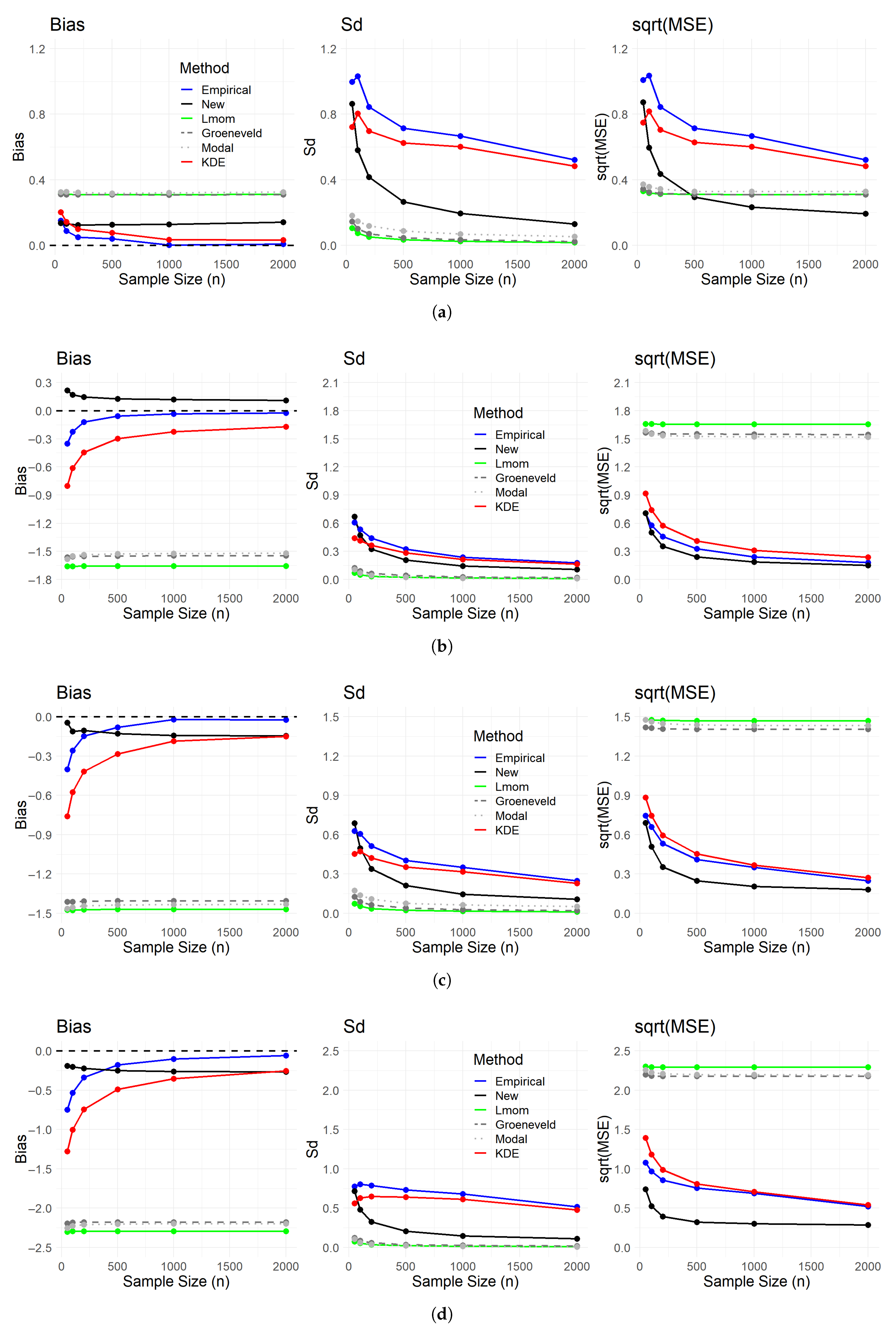
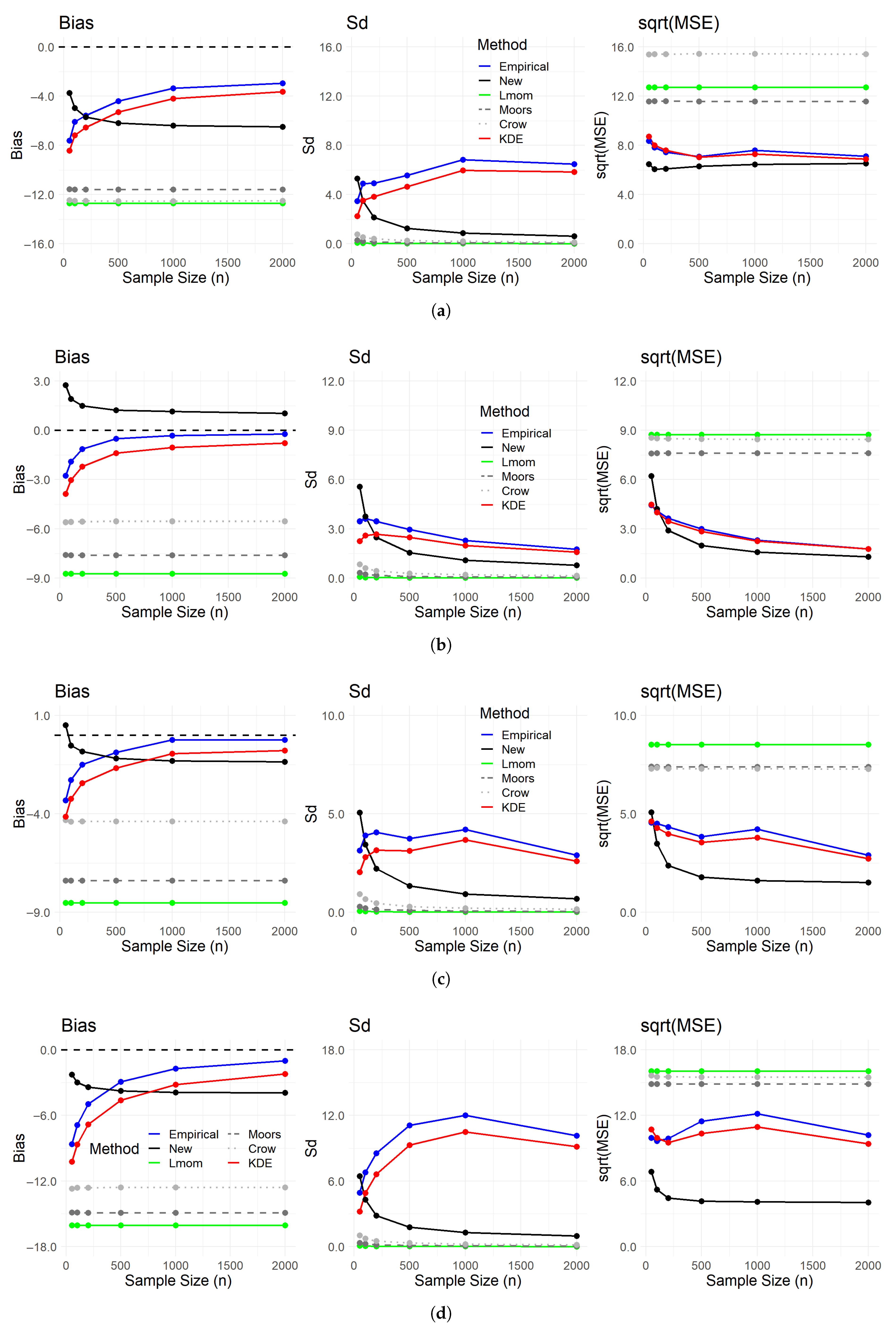
In all figures, we present only the better-performing estimators for clearer visual comparisons; see Supplementary Materials for the results of all methods used in our simulation. Figure 1 and Figure 2 show the results of the skewness and kurtosis estimation for the four standard distributions.
From the skewness results in Figure 1, we observe that the proposed estimator consistently outperforms existing methods across all considered distributions, with the exception of the symmetric t-distribution. Its superior performance is primarily attributable to enhanced bias correction, as evident from the simulation results. From a theoretical viewpoint, this bias correction is achieved through the flexibility of fitting a cubic polynomial in the standard normal quantile to the standardized data, allowing the method to adapt to a variety of distributional shapes. The advantage of this approach is particularly pronounced for asymmetric distributions such as in the case of LN and GPD, where conventional estimators tend to perform poorly. Notably, Empirical often ranks second under asymmetric distributions, reflecting the limitations of existing approaches in handling skewed datasets. The performance of KDE is similar to that of Empirical. The only exception to the proposed method’s strong performance is in estimating the skewness of the symmetric t-distribution. This is not surprising, as most existing estimators are designed to detect and quantify deviations from symmetry, as discussed in Section 2.7.
The kurtosis results shown in Figure 2 similarly indicate that the proposed estimator outperforms all competing methods, again due to its superior bias correction capabilities. Other existing estimators tend to underestimate true kurtosis, exhibiting negative bias that becomes gradually worse as tail heaviness increases, as seen in the case of GPD. Similarly to the skewness findings, the KDE estimator often ranks second in terms of MSE under asymmetric and heavy-tailed distributions, closely followed by Empirical. However, important contrasts emerge in the kurtosis results that distinguish them from the skewness findings. First, for the t-distribution, the proposed method now outperforms all other existing methods in kurtosis estimation, effectively capturing its heavy-tailed nature. Second, we observe that the standard deviation of the Empirical estimator increases with larger sample sizes when the underlying distribution is heavy-tailed (e.g., in the t-distribution and GPD), indicating a growing influence of outliers. In contrast, the proposed estimator exhibits decreasing standard deviations as the sample size increases, suggesting improved robustness to outliers.
Overall, Figure 1 and Figure 2 demonstrate that the proposed method offers substantial improvements over existing estimators for both skewness and kurtosis across a broad spectrum of distributions, with the only limitation being scenarios where the underlying distribution is perfectly symmetric. These findings highlight the practical utility of modeling standardized variables as cubic polynomials of the standard normal quantile, enabling flexible and accurate estimation of higher-order moments in the presence of asymmetry and heavy tails.
To assess the computational efficiency of the proposed regression-based estimator, we recorded the time required to complete 1000 simulations for varying sample sizes, using data generated from the scaled t-distribution; the results for other distributions were comparable. The findings, summarized in Table 2, demonstrate that the method is efficient across a wide range of sample sizes, with computation time increasing approximately linearly. These results confirm that the estimator scales well and remains computationally practical even for moderately large datasets.

4.2. Second Simulation Study

In practice, true data-generating processes in actuarial and insurance applications are rarely symmetric and often subject to contamination from various sources, making it difficult to characterize with a single distribution. To address this, we consider mixture models that combine two distributions. This mixture structure provides a more flexible approach to modeling the extreme volatility observed in financial data, allowing for a more accurate representation of tail risks compared to a single distribution. Specifically, for all distributions considered in the first simulation study above, we use a 95% weight on the distribution and introduce a G a m m a ( 2 ,   1 ) component with a 5% weight, except for the t-distribution, which uses another t-distribution, inspired by a Markov-switching model [35]. The true values of the mixture distributions were derived based on the moment calculation formula for mixture distributions, as given in [36]. As a result, the skewness and kurtosis of the mixture t-distribution were found to be −0.337 and 12.929, respectively, while those of the mixture G a m m a ( 2 ,   1 ) distribution were 1.6198 and 6.7959. For the mixture LN distribution, the values were 1.7 and 8.691, whereas the mixture GPD distribution had skewness and kurtosis values of 2.663 and 16.244, respectively. The results of the skewness and kurtosis estimation for the mixture distributions are presented in Figure 3 and Figure 4, respectively.
Regarding the skewness results in Figure 3, we can see that for the t-distribution, the New estimator now begins to outperform all existing methods from n = 500 onward, achieving the lowest MSE. This pattern can be explained as follows: When the sample size is small, the influence of the asymmetric component (5% of G a m m a ( 2 ,   1 ) distribution) is minimal, and the dataset from the mixture distribution remains approximately symmetric. As the sample size increases, however, the contribution of the gamma component becomes more substantial, gradually introducing asymmetry into the data. As a result, the proposed method increasingly performs better in capturing this skewness. For the other distributions, the New estimator consistently performs best across all sample sizes thanks to its ability to perform bias correction, similar to our first simulation study.
The kurtosis results in Figure 4 largely mirror those from the first simulation study, with the New estimator consistently outperforming existing methods across all mixture distributions considered. Taken together, these findings support the conclusion that the New estimator is both robust and effective in capturing skewness and kurtosis across a wide range of distributional settings commonly encountered in practice.

4.3. Analysis of Real Data

To examine and apply the proposed method to a real dataset, we analyze the daily closing prices of the S&P 500 index from 2 January 2008 to  29 December 2023. Daily returns are defined as the relative change in closing prices compared to the previous trading day and are calculated as
R t = P t P t 1 P t 1 ,
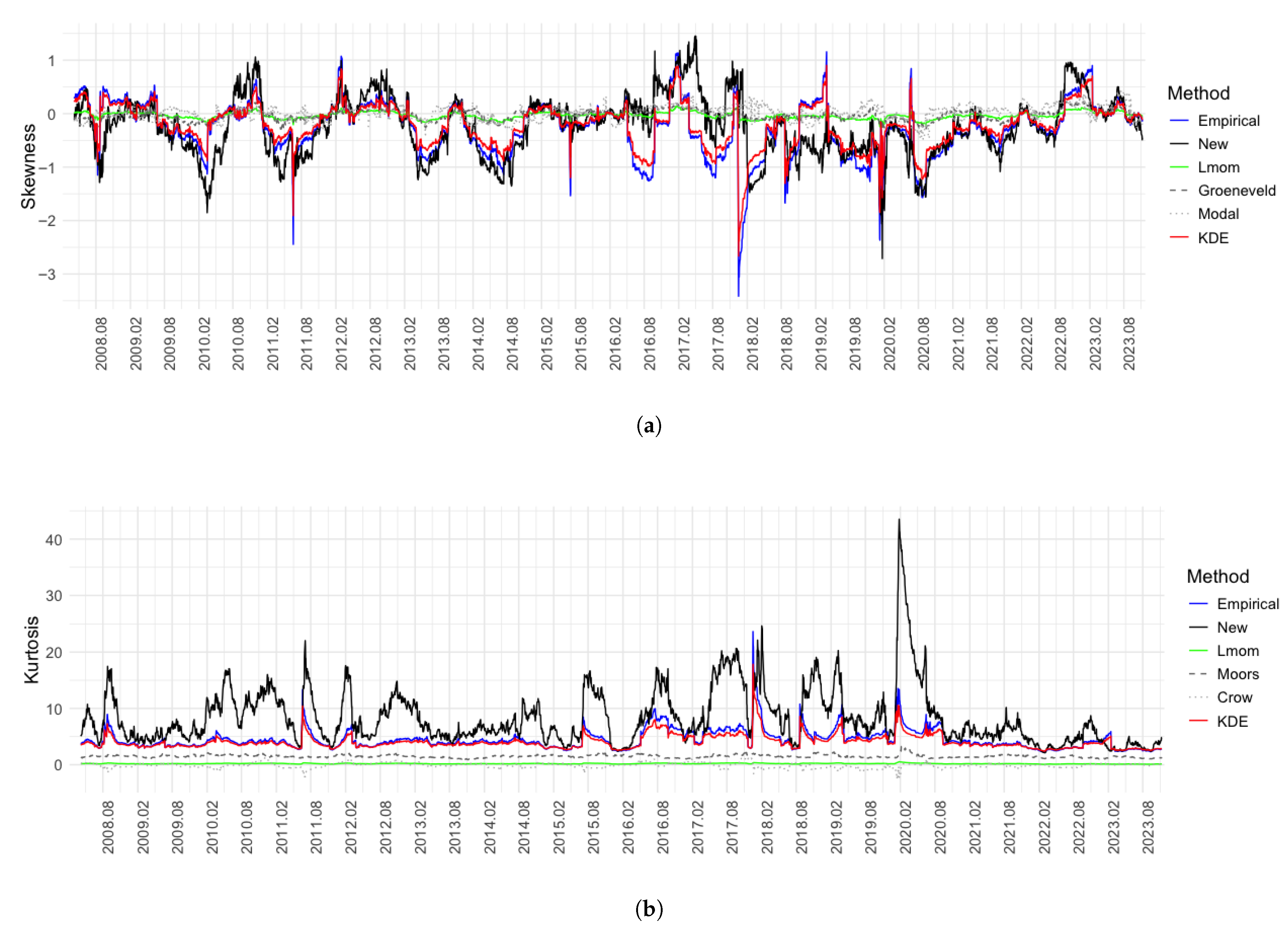
where P t denotes the closing price on day t. To examine the distributional characteristics of returns over time, at each time point, skewness and kurtosis are estimated using the methods described earlier with a rolling ±50-day window. This allows us to track the temporal dynamics of distributional asymmetry and tail behavior. The results are presented in Figure 5; for the results of the other estimators are in Supplementary Materials.
The skewness results in Figure 5a show that the New, Empirical, and KDE estimators are the most responsive to market changes. They consistently detect large negative skewness during turbulent market episodes, including the 2008–2009 financial crisis, the 2011 European debt crisis, the 2018 Volmageddon event (a sharp spike in market volatility that occurred in February 2018), and the early 2020 COVID-19 market crash. These three estimators largely move in tandem, but Empirical and KDE respond with somewhat smoother trajectories compared to the New estimator—except for the largest downside peak in early 2018, where the Empirical and KDE exhibit an extremely sharp drop. Another interesting point is that an extended period of positive skewness is observed for the New estimator, implying that more extreme positive returns were present during this period. The Empirical and KDE estimators do not show as strong a positive trend. Given that the S&P 500 index exhibited strong and stable growth over the 2016–2017 period, with relatively low volatility and no major drawdowns, these three estimators perform reasonably well.
In contrast, alternative estimators based on Lmom, Groeneveld, and Modal remain tightly centered around zero for much of the sample, with minimal response to extreme market conditions. This suggests that such methods may be insufficiently sensitive to capture shifts in asymmetry during high-volatility or crisis periods, which are common in financial return series. Overall, the evidence from the figure confirms that the New and KDE estimators offer the most informative and responsive tracking of skewness dynamics in equity markets. While Empirical skewness also provides meaningful signals, it is more volatile and less robust to short-term outliers. The KDE estimator, as a nonparametric density-based alternative, demonstrates that ML-inspired smoothers can offer practical benefits in higher-moment estimation.
We now turn to the kurtosis results, as shown in Figure 5b. As with skewness, the three estimators—New, Empirical, and KDE—display the highest sensitivity to tail behavior and outliers, particularly during periods of systemic risk. In particular, for the New estimator, kurtosis spikes are most pronounced and clearly visible during major events: the global financial crisis (2008–2009), the 2010–2011 sovereign debt crises, the 2015–2016 global slowdown, the 2018 volatility shock, and the COVID-19 crash in early 2020. The New estimator registers peaks well above 20—and in some cases exceeding 40—reflecting extreme tail risk and leptokurtic behavior. The KDE estimator once again closely mirrors the general pattern of the Empirical method, albeit with smoother peaks and slightly lower amplitude.
In stark contrast, kurtosis estimators based on Lmom, Moors, and Crow remain flat throughout the entire sample period. These estimators fail to detect any of the documented volatility regimes, consistently returning values near or below 3—the benchmark for normality. This under-responsiveness highlights their limited suitability for financial applications, particularly in contexts where accurate tail modeling is critical for risk assessment and stress testing.

5. Conclusions

This paper proposes a new, robust method for the joint estimation of skewness and kurtosis in datasets that are asymmetric and heavy-tailed—features commonly observed in actuarial and financial applications. Estimating these higher-order moments is a foundational problem in statistical analysis, particularly in the context of insurance risk management, portfolio allocation, and financial modeling. Despite its long-standing significance, the accurate estimation of these moments remains an unresolved challenge. Traditional moment-based estimators, while analytically convenient, are highly sensitive to outliers and often yield misleading results when applied to non-normal distributions. Although numerous alternatives have been developed over the years—including robust L-moment techniques and quantile-based measures—many of these approaches are constrained by narrow output ranges, limited responsiveness to extreme observations, or an implicit assumption of near-symmetric distributions, reducing their effectiveness in practical, real-world settings.
To address these limitations, we introduce a regression-based estimator derived from the Cornish–Fisher (CF) expansion and implemented via median regression on the quantile space of the standard normal distribution. This approach offers a flexible, data-driven alternative that mitigates the instability of moment-based methods while enhancing robustness and interpretability in applied settings. For this we model the standardized empirical data as a cubic polynomial function of the standard normal quantile under a regression framework. This structure confers several key advantages. First, it eliminates the need to use higher-order sample moments, which are often volatile and unreliable, by capturing the distributional shape through estimated polynomial coefficients. Second, the use of median regression reduces sensitivity to outliers and ensures monotonicity of the fitted quantile function—an important property frequently violated in conventional truncated CF approximations. From the fitted regression function, we derive closed-form expressions for skewness and kurtosis, enabling accurate and efficient joint estimation of these higher-order moments for the original dataset. The flexibility of the polynomial form further enables approximation of a wide variety of distributional shapes without imposing strong parametric assumptions, making the method broadly applicable to complex, real-world data.
Extensive simulation studies show the superior performance of the proposed method across a wide range of distributions and various mixture models. The method consistently outperforms existing moment-based and quantile-based estimators in terms of both mean squared error and bias, particularly under asymmetric and heavy-tailed conditions. However, we find that if the underlying distribution is multimodal or the sample size is relatively small (e.g., fewer than 20 observations), the estimator’s performance may deteriorate as it has insufficient information to reliably estimate the coefficients of median regression. From a practical standpoint, the estimator offers a valuable tool for risk management, financial modeling, and solvency assessments, where accurate characterization of distributional asymmetry and tail behavior is essential. Its ability to operate without strong distributional assumptions makes it particularly attractive for applied contexts where model uncertainty is high.

Supplementary Materials

The following supporting information can be downloaded at: https://www.mdpi.com/article/10.3390/math13162694/s1, Table S1: Simulation results; Table S2: S&P results.

Author Contributions

Conceptualization, J.H.T.K.; methodology, J.H.T.K.; software (R 4.4.1), H.K.; validation, H.K.; formal analysis, J.H.T.K. and H.K.; investigation, J.H.T.K.; resources, H.K.; data curation, J.H.T.K.; writing—original draft preparation, J.H.T.K. and H.K.; writing—review and editing, J.H.T.K.; visualization, H.K.; supervision, J.H.T.K.; project administration, J.H.T.K.; funding acquisition, J.H.T.K. All authors have read and agreed to the published version of the manuscript.

Funding

This work was supported by the Ministry of Education of the Republic of Korea (2022S1A5A2A03052219) and the National Research Foundation of Korea (2022R1F1A106357511).

Data Availability Statement

The R code used to implement the proposed estimator is available at https://github.com/jhtkim2012/Regression-based-skewness-and-kurtosis-estimation (accessed on 10 August 2025).

Acknowledgments

The authors thank the editors and the anonymous reviewers for their helpful comments, which improved the readability and quality of this manuscript.

Conflicts of Interest

The authors declare no conflicts of interest.

Appendix A

  • T t ν , Student’s t-distribution with degrees of freedom ν , has a density of
    f ( t ) = Γ ( ν + 1 2 ) π ν Γ ( ν 2 ) 1 + t 2 ν ( ν + 1 ) / 2
    E ( T ) = 0 ; V a r ( T ) = ν ν 2
    The scaled t-distribution, denoted by X, is a location-scale transformation of the standard Student’s t-distribution. That is, X = μ + σ T , so that
    E ( X ) = μ ; V a r ( X ) = ν ν 2 σ 2
  • X G a m m a ( k , θ ) has a density of
    f ( x ) = x k 1 e x θ θ k Γ ( k ) for x > 0 and k , θ > 0
    E ( X ) = k θ ; V a r ( X ) = k θ 2
  • X L N μ , σ 2 has a density of
    f X ( x ) = 1 x σ 2 π exp ( ln x μ ) 2 2 σ 2 for x > 0
    E ( X ) = exp μ + σ 2 2 ; V a r ( X ) = e σ 2 1 exp ( 2 μ + σ 2 )
  • X G P D ( ξ , σ ) has a density, for ξ > 0 , of
    f ( x ) = 1 σ 1 + ξ σ x 1 / ξ 1 , x > 0
    E ( X ) = σ 1 ξ ; V a r ( X ) = σ 2 ( 1 ξ ) 2 ( 1 2 ξ )

References

  1. Harvey, C.R.; Siddique, A. Conditional skewness in asset pricing tests. J. Financ. 2000, 55, 1263–1295. [Google Scholar] [CrossRef]
  2. Hwang, S.; Satchell, S.E. Modelling emerging market risk premia using higher moments. Int. J. Financ. Econ. 1999, 4, 271–296. [Google Scholar] [CrossRef]
  3. Jorion, P. On jump processes in the foreign exchange and stock markets. Rev. Financ. Stud. 1988, 1, 427–445. [Google Scholar] [CrossRef]
  4. Sandström, A. Solvency II: Calibration for skewness. Scand. Actuar. J. 2007, 126–134. [Google Scholar] [CrossRef]
  5. Brys, G.; Hubert, M.; Struyf, A. A comparison of some new measures of skewness. In Developments in Robust Statistics: International Conference on Robust Statistics 2001; Springer: Berlin/Heidelberg, Germany, 2003; pp. 98–113. [Google Scholar]
  6. Bates, D.S. Jumps and stochastic volatility: Exchange rate processes implicit in deutsche mark options. Rev. Financ. Stud. 1996, 9, 69–107. [Google Scholar] [CrossRef]
  7. Bonato, M. Robust estimation of skewness and kurtosis in distributions with infinite higher moments. Financ. Res. Lett. 2011, 8, 77–87. [Google Scholar] [CrossRef]
  8. Kim, T.-H.; White, H. On more robust estimation of skewness and kurtosis. Financ. Res. Lett. 2004, 1, 56–73. [Google Scholar] [CrossRef]
  9. Bastianin, A. Robust measures of skewness and kurtosis for macroeconomic and financial time series. Appl. Econ. 2020, 52, 637–670. [Google Scholar] [CrossRef]
  10. Groeneveld, R.A.; Meeden, G. Measuring skewness and kurtosis. J. R. Stat. Soc. Ser. D Stat. 1984, 33, 391–399. [Google Scholar] [CrossRef]
  11. Klugman, S.A.; Panjer, H.H.; Willmot, G.E. Loss Models, 3rd ed.; John Wiley: New York, NY, USA, 2008. [Google Scholar]
  12. Sandström, A. Handbook of Solvency for Actuaries and Risk Managers: Theory and Practice; CRC Press: Boca Raton, FL, USA, 2011. [Google Scholar]
  13. van Broekhoven, H. Market value of liabilities mortality risk: A practical model. North Am. Actuar. J. 2002, 6, 95–106. [Google Scholar] [CrossRef]
  14. Hosking, J.R.M. L-moments: Analysis and estimation of distributions using linear combinations of order statistics. J. R. Stat. Soc. Ser. B Stat. Methodol. 1990, 52, 105–124. [Google Scholar] [CrossRef]
  15. Zhao, Y.-G.; Tong, M.-N.; Lu, Z.-H.; Xu, J. Monotonic expression of polynomial normal transformation based on the first four L-moments. J. Eng. Mech. 2020, 146, 06020003. [Google Scholar] [CrossRef]
  16. Elamir, E.A.H.; Seheult, A.H. Trimmed L-moments. Comput. Stat. Data Anal. 2003, 43, 299–314. [Google Scholar] [CrossRef]
  17. Bowley, A.L. Elements of Statistics; P. S. King & Son: London, UK, 1926. [Google Scholar]
  18. Crow, E.L.; Siddiqui, M.M. Robust estimation of location. J. Am. Stat. Assoc. 1967, 62, 353–389. [Google Scholar] [CrossRef]
  19. Kendall, M.G.; Stuart, A. The Advanced Theory of Statistics; Griffin: London, UK, 1977; Volume 1. [Google Scholar]
  20. Moors, J.J.A. A quantile alternative for kurtosis. J. R. Stat. Soc. Ser. D (Stat.) 1988, 37, 25–32. [Google Scholar] [CrossRef]
  21. Brys, G.; Hubert, M.; Struyf, A. A robust measure of skewness. J. Comput. Graph. Stat. 2004, 13, 996–1017. [Google Scholar] [CrossRef]
  22. Bickel, D.R. Robust estimators of the mode and skewness of continuous data. Comput. Stat. Data Anal. 2002, 39, 153–163. [Google Scholar] [CrossRef]
  23. Hogg, R.V. More light on the kurtosis and related statistics. J. Am. Stat. Assoc. 1972, 67, 422–424. [Google Scholar] [CrossRef]
  24. Hogg, R.V. Adaptive robust procedures: A partial review and some suggestions for future applications and theory. J. Am. Stat. Assoc. 1974, 69, 909–923. [Google Scholar] [CrossRef]
  25. Cornish, E.A.; Fisher, R.A. Moments and cumulants in the specification of distributions. Rev. L’Inst. Int. Stat. 1938, 5, 307–320. [Google Scholar] [CrossRef]
  26. Johnson, N.L.; Kotz, S.; Balakrishnan, N. Continuous Multivariate Distributions, Volume 1: Models and Applications; John Wiley & Sons: New York, NY, USA, 2002. [Google Scholar]
  27. Aboura, S.; Maillard, D. Option pricing under skewness and kurtosis using a Cornish–Fisher expansion. J. Futur. Mark. 2016, 36, 1194–1209. [Google Scholar] [CrossRef]
  28. Ruiz-Rodriguez, F.J.; Hernández, J.C.; Jurado, F. Probabilistic load flow for photovoltaic distributed generation using the Cornish–Fisher expansion. Electr. Power Syst. Res. 2012, 89, 129–138. [Google Scholar] [CrossRef]
  29. Zangari, P. A VaR methodology for portfolios that include options. RiskMetrics Monit. 1996, 1, 4–12. [Google Scholar]
  30. Zhao, Y.-G.; Lu, Z.-H. Cubic normal distribution and its significance in structural reliability. Struct. Eng. Mech. 2008, 28, 263–280. [Google Scholar] [CrossRef]
  31. Amédée-Manesme, C.-O.; Barthélemy, F.; Maillard, D. Computation of the corrected Cornish–Fisher expansion using the response surface methodology: Application to VaR and CVaR. Ann. Oper. Res. 2019, 281, 423–453. [Google Scholar] [CrossRef]
  32. Kim, H.; Kim, J.; Kim, J.H.T. A new skewness adjustment for Solvency II SCR standard formula. Scand. Actuar. J. 2025, in press. [Google Scholar] [CrossRef]
  33. Koenker, R. Quantile Regression; Vol. 38, Econometric Society Monographs; Cambridge University Press: Cambridge, UK, 2005. [Google Scholar]
  34. Jondeau, E.; Poon, S.-H.; Rockinger, M. Financial Modeling Under Non-Gaussian Distributions; Springer Science & Business Media: Berlin/Heidelberg, Germany, 2007. [Google Scholar]
  35. Hardy, M. Investment Guarantees; John Wiley & Sons: Hoboken, NJ, USA, 2003. [Google Scholar]
  36. Frühwirth-Schnatter, S. Finite Mixture and Markov Switching Models; Springer: Berlin/Heidelberg, Germany, 2006. [Google Scholar]
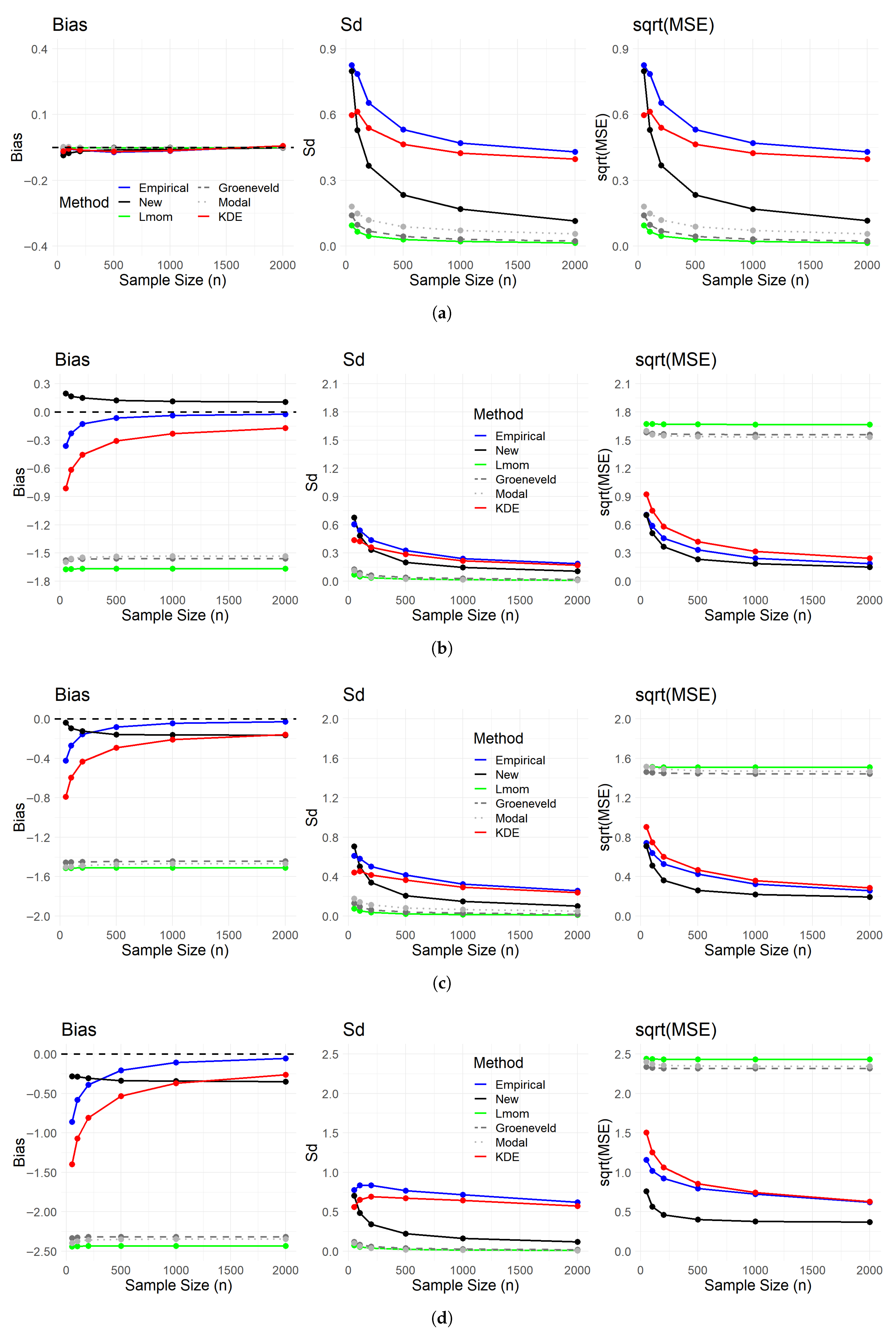
Figure 1. Skewness results. (a) t 5 with true value of 0.00. (b) G a m m a ( 1 ,   1 ) with true value of 2.00. (c) LN ( 1 ,   0.5 2 ) with true value of 1.75. (d) GPD ( 0.1 ,   2 ) with true value of 2.811.
Mathematics 13 02694 g001
Figure 2. Kurtosis results. (a) t 5 with true value of 9.00. (b) G a m m a ( 1 ,   1 ) with true value of 9.00. (c) LN ( 1 ,   0.5 2 ) with true value of 8.898. (d) GPD ( 0.1 ,   2 ) with true value of 17.829.
Mathematics 13 02694 g002
Figure 3. Skewness results for mixture distributions. (a) t 5 mixture with true value of 0.337 . (b) G a m m a ( 1 ,   1 ) mixture with true value of 1.6198. (c) LN ( 1 ,   0.5 2 ) mixture with true value of 1.7. (d) GPD ( 0.1 ,   2 ) mixture with true value of 2.663.
Mathematics 13 02694 g003
Figure 4. Kurtosis results for mixture distributions. (a) t 5 mixture with true value of 12.929 . (b) G a m m a ( 1 ,   1 ) mixture with true value of 6.7959 (c) LN ( 1 ,   0.5 2 ) mixture with true value of 8.691. (d) GPD ( 0.1 ,   2 ) mixture with true value of 16.244.
Mathematics 13 02694 g004
Figure 5. Skewness and kurtosis results for S&P daily returns. (a) Estimated skewness using different methods. (b) Estimated kurtosis using different methods.
Mathematics 13 02694 g005
Table 1. Summary statistics for the distributions.
DistributionMeanVarianceSkewnessKurtosis
t 5 (scaled)9.556127.8609
G a m m a ( 1 , 1 ) 1129
L N ( 1 , 0.5 2 ) 3.082.691.758.898
G P D ( 0.1 , 2 ) 2.226.172.81117.829
Table 2. Computation time for 1000 simulations under the scaled t-distribution. Hardware: Apple Mac Studio (M2 Max, 64 GB RAM); software: R version 4.4.1.
Sample Size (n)Time (Seconds)
501.86
1002.43
2003.67
5006.79
100011.96
200023.10
Disclaimer/Publisher’s Note: The statements, opinions and data contained in all publications are solely those of the individual author(s) and contributor(s) and not of MDPI and/or the editor(s). MDPI and/or the editor(s) disclaim responsibility for any injury to people or property resulting from any ideas, methods, instructions or products referred to in the content.