Abstract
High dynamic range (HDR) tone mapping techniques have been widely studied to effectively represent the broad dynamic range of real-world scenes. However, generating an HDR image from multiple low dynamic range (LDR) images captured at different exposure levels can introduce ghosting artifacts in dynamic scenes. Moreover, methods that estimate HDR information from a single LDR image often suffer from inherent accuracy limitations. To overcome these limitations, this study proposes a novel image processing technique that extends the dynamic range of a single LDR image. This technique achieves the goal through leveraging a Convolutional Neural Network (CNN) to generate a synthetic Near-Infrared (NIR) image—one that emulates the characteristic of real NIR imagery being less susceptible to diffraction, thus preserving sharper outlines and clearer details. This synthetic NIR image is then fused with the original LDR image, which contains color information, to create a tone-distributed HDR-like image. The synthetic NIR image is produced using a lightweight U-Net-based autoencoder, where the encoder extracts features from the LDR image, and the decoder synthesizes a synthetic NIR image that replicates the characteristics of a real NIR image. To enhance feature fusion, a cardinality structure inspired by Extended-Efficient Layer Aggregation Networks (E-ELAN) in You Only Look Once Version 7 (YOLOv7) and a modified convolutional block attention module (CBAM) incorporating a difference map are applied. The loss function integrates a discriminator to enforce adversarial loss, while VGG, structural similarity index, and mean squared error losses contribute to overall image fidelity. Additionally, non-reference image quality assessment losses based on BRISQUE and NIQE are incorporated to further refine image quality. Experimental results demonstrate that the proposed method outperforms conventional HDR techniques in both qualitative and quantitative evaluations.
MSC:
68T45
1. Introduction
The real world exhibits a wide dynamic range, but camera sensors and display devices have inherent limitations in capturing and reproducing the full spectrum of brightness and color information present in natural environments. While increasing the dynamic range of camera sensors and display devices can mitigate information loss, physically enhancing sensor capabilities is costly. To address this issue, high dynamic range (HDR) imaging technology has been developed, enabling the synthesis of multiple images with limited dynamic ranges to preserve more visual information [1,2]. In HDR imaging, a camera’s exposure value (EV) determines the amount of light reaching the sensor. A low EV captures details in bright areas, whereas a high EV preserves details in dark regions but leads to saturation in bright areas. However, when capturing dynamic scenes, this approach introduces motion artifacts, resulting in ghosting effects. To overcome these limitations, research has explored methods for empirically estimating HDR information from a single low dynamic range (LDR) image [3,4]. These methods primarily reconstruct lost luminance information through empirical modeling but struggle to accurately restore saturated regions. Overcoming the challenges posed by dynamic scenes, the difficulty of acquiring multiple LDR images in static environments, and the accurate reconstruction of lost information from a single LDR image remains a significant challenge.
NIR imaging captures light in the wavelength range of approximately 700–1000 nm. Compared to visible light images, NIR exhibits a property of reduced diffraction due to its longer wavelength. Furthermore, NIR images demonstrate higher contrast and provide richer texture details that are less perceptible in the visible spectrum. This is attributed to NIR imaging more effectively emphasizing object reflectance characteristics than visible imaging, which enhances the distinguishability of object materials. These inherent properties manifest a pronounced tone compression effect within NIR images, enabling visually more nuanced and richer representational capabilities. Specifically, NIR imaging highlights variations in the reflectance of biological materials such as vegetation and human skin, making it useful for applications such as vegetation analysis and forgery detection [5,6,7]. Additionally, due to their strong contrast and high boundary separation properties, NIR images enhance visibility in challenging environments with fog, dust, and smoke, improving detail restoration, noise reduction, and texture enhancement [8,9]. Conventional multi-band image fusion (VIS-NIR) leverages the characteristics of NIR images, particularly their tone compression effect in the luminance (L) channel [10,11]. However, traditional multi-band fusion techniques require capturing the same scene with multiple cameras, which introduces ghosting artifacts in dynamic scenes and complicates data acquisition—issues similar to those faced in multi-exposure HDR synthesis.
The rapid advancement of deep neural networks, driven by improvements in computing power, storage capacity, and network architectures, has led to significant progress in image processing research. Inspired by the primate visual cortex, deep neural network architectures have proven highly effective for image-to-image translation tasks, including HDR reconstruction from LDR images [12,13]. Early convolutional neural networks (CNNs) were often considered “black boxes,” making their outputs difficult to interpret. However, recent studies have analyzed CNN architectures in terms of width, depth, and cardinality to improve network efficiency [14]. Moreover, the introduction of attention mechanisms has further enhanced training efficiency by guiding feature learning more effectively [15,16]. Building upon the strengths of conventional VIS-NIR fusion, this study proposes a virtual multi-band image fusion method that generates a synthetic NIR image from a single visible (RGB) image and integrates it for HDR image synthesis. The proposed approach consists of two main stages:
- Synthetic NIR Image Generation: A lightweight U-Net-based autoencoder generates a synthetic NIR image that replicates the characteristics of real NIR images. The encoder extracts features from the input visible image, while the decoder synthesizes the synthetic NIR image in the latent space.
- Image Fusion and Enhancement: The synthetic NIR image and the visible image are fused using a synthesis module. To maximize encoder performance, an Expand, Shuffle, and Merge Cardinality structure, inspired by YOLOv7’s E-ELAN, expands the CNN’s width and depth. Additionally, a Modified Convolutional Block Attention Module (CBAM) incorporating a Difference Map (diff-CBAM) is applied to emphasize key regions during learning.
The encoder consists of five blocks, each integrating the cardinality structure and diff-CBAM, while the decoder comprises two layers and five diff-CBAMs. Both components employ a bottleneck structure to compress and reconstruct image data effectively. To optimize image quality, a discriminator is added to apply adversarial loss, while the training process incorporates VGG loss, structural similarity index (SSIM) loss, and mean squared error (MSE) loss. Additionally, non-reference image quality assessment (IQA) metrics such as BRISQUE and NIQE are used as loss functions to enhance learning. Overall, adversarial loss, VGG loss, SSIM loss, MSE loss, BRISQUE loss, and NIQE loss collectively optimize the network. The contributions of this work are as follows:
- A two-step process is proposed, where a synthetic NIR image is first generated to replicate NIR characteristics and then fused with a visible image to enhance HDR synthesis.
- Experimental results confirm that the first-stage training effectively learns NIR characteristics from visible images, enabling the generation of high-quality synthetic NIR images.
- The second-stage training demonstrates that incorporating NIR characteristics significantly improves HDR synthesis efficiency. Additionally, a lightweight architecture, combined with cardinality and attention mechanisms, optimizes the module structure while reducing computational complexity.
The remainder of this paper is structured as follows: Section 2 provides background knowledge relevant to this study. Section 2.1 reviews traditional HDR methods, covering both single-image HDR techniques and multi-image HDR approaches. Section 2.2 introduces image processing with CNNs, including the Extended Efficient Layer Aggregation Network and the Convolutional Block Attention Module. Section 3 details the proposed method. Section 3.1 explains the generation of synthetic NIR images, and Section 3.2 describes the process of enhancing image quality by fusing synthetic NIR images with visible images. Section 4 presents experimental validation. Section 4.1 demonstrates visual improvements through qualitative comparisons, while Section 4.2 quantitatively evaluates performance using NR-IQA metrics. Graphs and tables are included for intuitive presentation. Section 5 concludes the study and summarizes the findings.
2. Related Works
Displays have a limited range of luminance and chroma compared to the human visual system. Consequently, areas that are distinguishable to the human eye, such as bright and dark regions, may appear overly bright or dark when captured by a camera and displayed. This can lead to information loss, depending on exposure settings and display performance. To address this issue, this study explores a method for estimating HDR images from a single LDR image using CNNs. This section discusses both traditional HDR techniques and CNN-based HDR tone-mapping approaches.
2.1. Traditional HDR Methods
HDR image processing seeks to overcome the limitations of standard LDR images by minimizing the loss of overexposed bright areas and underexposed dark areas. One commonly used method involves combining multiple images captured at different exposure levels to reconstruct a high-quality HDR image. However, this approach faces challenges when processing dynamic scenes, as motion artifacts may occur. To address the limitations of multi-exposure HDR techniques, single-image HDR methods have been developed to recover HDR information from a single LDR image. These methods typically rely on empirical techniques to estimate lost luminance information, though they struggle to accurately restore fully saturated areas. Section 2.1.1 discusses techniques for recovering HDR information from a single-exposure LDR image, while Section 2.1.2 covers research on HDR image generation based on multiple exposures and multi-band approaches.
2.1.1. Single Information-Based HDR
Single-exposure HDR techniques, based on mathematical models or empirical methods, aim to extend the dynamic range by estimating the luminance information of the image. These methods primarily seek to restore lost details and enhance information in both bright and dark regions using specific algorithms. Kwon et al. propose a novel surround map that addresses the complexities of detail-based separation and multi-scale techniques, reduces halo artifacts in single-scale processing, and enhances detail restoration [17]. Kim et al. combine the Retinex theory with multi-scale contrast-limited adaptive histograms to reduce halo artifacts and detail loss during the tone-mapping process [18]. iCAM06 is an image representation model that enhances contrast and color representation of HDR images by applying a spatial processing model of the human visual system and its light adaptation functions [19]. Reinhard et al. introduce a new operator for tone reproduction in digital images, inspired by photographic practices. Their algorithm effectively compresses HDR information while avoiding information loss during linear scaling [20]. The L1L0 method uses a decomposition model to separate the base and detail layers, applying appropriate sparsity terms to each layer to solve halo artifacts and over-enhancement issues in tone mapping [21]. Lee et al. propose a method to generate HDR images from a single LDR image using HSVNet, a U-Net-based CNN architecture that utilizes the HSV color space [22]. Unlike multi-exposure HDR methods, these mathematical and empirical approaches do not suffer from phenomena like ghosting in dynamic scenes, making them easier to capture. However, they still face challenges in perfectly restoring details in overly bright or dark regions, and estimating lost information in LDR images may not guarantee perfect results if the scene is complex or the video is unstable.
2.1.2. Multi-Information Based HDR
Multi-exposure HDR techniques generate HDR images with a wider dynamic range by combining multiple LDR images captured at different exposure levels. In this method, several images of the same scene are captured with varying exposure times to collect LDR images that preserve information in both bright and dark areas. Images captured with shorter exposure times retain details in the bright areas, while those with longer exposure times capture information in the darker regions. These images complement each other to create a single HDR image. An et al. improve the multi-exposure HDR fusion algorithm by introducing new weights that reflect contrast, saturation, and optimal exposure, effectively reducing ghosting artifacts. Their experiments demonstrate that this approach successfully removes ghosting and artifacts compared to existing methods [23]. Merianos et al. propose an HDR imaging algorithm using low-cost image sensors, combining the luminance channel using Mitianoudis et al.’s method and the color channels using Mertens et al.’s approach, to address multi-exposure fusion issues [24,25,26]. Jinno et al. suggest a method for simultaneously estimating image displacement, occlusion, and saturation areas while preventing motion blur and ghosting artifacts during HDR image creation [1]. Hu et al. propose a lightweight framework for HDR image reconstruction that generates and fuses multiple images based on exposure bias estimation and contrast enhancement, enabling robust high-quality HDR synthesis under diverse lighting conditions [27].
In addition to synthesizing LDR images with varying exposure levels, there has been research on fusing images from different bands, such as visible and infrared (IR) images. IR images emphasize the reflective properties of objects, often leading to tone compression effects. Son et al. combine visible and IR images using contour transformation, principal component analysis, and iCAM06, effectively merging the color information of visible images with the detail from NIR images [28]. Lee et al. propose an algorithm for fusing NIR and visible images by adjusting the detail and base information using a just noticeable difference (JND) profile, providing better texture information and contrast adjustments [11]. Kwon et al. demonstrate a method for combining infrared and visible images using depth-weighted radiance maps to enhance local contrast, applying luminance blending, tone mapping, and color correction [29]. These multi-exposure and multi-band HDR methods combine images captured with different exposure values and spectral bands to provide a broader dynamic range and greater detail. However, during multi-exposure capturing, if the subject moves, image alignment may be imperfect, leading to ghosting artifacts in the fusion process. Moreover, since multiple captures of the same scene are required, this method necessitates a camera capable of supporting such operations and additional computational efforts for image alignment and correction.
2.2. Image Processing with CNN
A typical CNN architecture consists of convolutional layers, pooling layers, fully connected layers, and activation functions. The convolutional layers focus on specific regions of the input image to generate feature maps, enabling the network to learn spatial hierarchies of patterns. Pooling layers perform down-sampling, reducing computational complexity while preserving critical information. This allows the network to extract both global and high-level features by maintaining a fixed window size. Fully connected layers, typically located at the network’s end, generate final classification or regression outputs. Activation functions apply non-linear transformations to the outputs of neurons, addressing issues like vanishing gradients and allowing the model to learn complex patterns in the data.
CNN architecture has evolved to optimize three key factors—width, depth, and cardinality—which significantly enhance feature extraction capabilities. Depth refers to the number of layers in the network. Deeper architectures can learn more complex and hierarchical features. Notable deep neural networks such as VGG-16 and ResNet have shown performance improvements with increased depth [30,31]. However, overly deep networks may suffer from vanishing gradients and high computational costs, which can degrade learning efficiency and hinder generalization. Width refers to the number of filters used in each layer. Wider networks can extract a broader range of features. For example, the Wide ResNet model enhances learning capacity by increasing the network’s width instead of depth [32]. Cardinality involves the number of filter groups processed in parallel within each layer. Increasing cardinality improves the network’s representational power while maintaining computational efficiency. ResNet demonstrated that increasing cardinality enhances representational capacity without compromising computational efficiency [33].
The following sections provide a detailed explanation of the structures utilized in the proposed method. Section 2.2.1 discusses the extended efficient layer aggregation network (E-ELAN), while Section 2.2.2 explains the CBAM.
2.2.1. Extended Efficient Layer Aggregation Network
E-ELAN extends the original ELAN architecture to maximize the network’s learning capabilities while minimizing computational costs. This structure incorporates cardinality to enhance parallel learning, optimizing various depths and widths within the network. Rather than merely increasing the network’s depth and width, E-ELAN leverages parallel pathways to maximize performance improvements without incurring significant computational overhead. Furthermore, E-ELAN introduces expansion, shuffle, and merge cardinality to enhance the network’s representational power while preserving the gradient path and improving overall performance. Expansion cardinality increases the number of channels in computational blocks, enabling the network to learn diverse features. Shuffle cardinality divides feature maps into multiple groups and shuffles them to optimize information distribution, facilitating the learning of varied patterns. Merge cardinality integrates the feature map groups learned in parallel, further strengthening the network’s representational capacity. This cardinality adjustment strategy enables E-ELAN to effectively learn diverse features while maintaining stability in learning and improving performance. Compared to simply increasing network depth, this approach offers a more efficient method of optimizing parallel learning and expanding the network’s representational capacity [34,35].
2.2.2. Convolutional Block Attention Module
The CBAM is a module designed to improve CNN performance by combining channel-wise and spatial attention mechanisms to highlight important features while suppressing irrelevant information [15]. This module enables the network to focus on key areas of the input feature map, as illustrated in Figure 1.
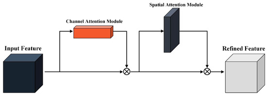
Figure 1.
Architecture of the convolutional block attention module.
The channel attention module in CBAM learns the inter-channel relationships of the input feature map, highlighting the most important channels. This is achieved by performing average pooling and max pooling along the spatial dimension to generate two 1-dimensional vectors. These vectors are passed through a multilayer perceptron (MLP), which produces the channel attention map. The input feature map is then element-wise multiplied by the channel attention map, enabling the network to focus on the most relevant features.
The spatial attention module follows, using spatial location information to emphasize important regions of the feature map. Average pooling and max pooling are applied along the channel dimension, and the resulting feature maps are concatenated. A 7 7 convolution is then applied to generate the spatial attention map, helping the network focus on the “where” of the important regions. By sequentially applying these channel and spatial attention modules, CBAM refines the input feature map, enhancing the network’s expressiveness with minimal computational cost and low structural complexity. The operating principles of the channel attention module and spatial attention module of CBAM are represented by the following equations:
where and represent the channel and spatial attention modules, respectively; denotes the feature map; refers to the MLP; and indicates a convolution operation with a filter size of .
3. Proposed Method
This study presents a virtual multi-band image fusion method that utilizes the tone compression characteristics of NIR images in the fusion process of real visible and NIR images. The proposed approach is based on a CNN-based learning framework and consists of two key stages. First, a synthetic NIR image, which captures the characteristics of real NIR images, is generated from a single LDR visible image using CNN training. Then, the generated synthetic NIR image is fused with the original LDR image through an additional CNN training process to produce an HDR image. The learning process is divided into two stages. In the first stage, a synthetic NIR image is generated from the input visible image. In the second stage, the synthetic NIR image is fused with the original visible image to produce an HDR image. During inference, only a single visible image is required as input. The module trained in the first stage generates a Synthetic NIR image, while the module trained in the second stage fuses the synthetic NIR image with the visible image to produce the final HDR output. The overall workflow is illustrated in Figure 2.
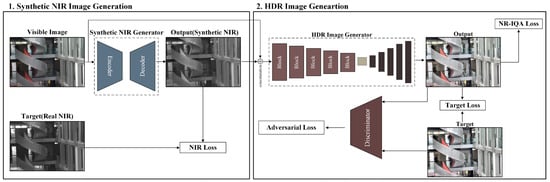
Figure 2.
Flow chart of the proposed method.
As shown in Figure 2, the first stage of training involves generating a synthetic NIR image. A visible image is provided as input to an encoder-decoder module, which is trained using real NIR images as targets. The training process minimizes the difference between the generated synthetic NIR image and the target real NIR image using a loss function. The resulting synthetic NIR image is then concatenated with the original visible image, forming a four-channel tensor dataset that serves as input for the next stage.
In the second training stage, the four-channel tensor dataset is processed by another encoder-decoder module to generate an HDR image. The encoder extracts meaningful features from the input data, which consists of both visible and synthetic NIR images. To enhance feature extraction, the encoder incorporates five blocks that integrate elements from CBAM’s channel and spatial attention modules and Extend, Shuffle, and Merge cardinality operations from the E-ELAN structure in YOLOv7. The training process employs adversarial loss with a discriminator, loss functions that measure the error between the generated and target images, and NR-IQA metrics as learning objectives. Section 3.1 and Section 3.2 provide detailed explanations of the training processes for the first and second stages, respectively.
3.1. Synthetic NIR Image Generation
NIR imaging effectively captures reflectance and thermal characteristics by utilizing the NIR spectrum, revealing surface features that are often difficult to detect in visible images. This capability enables NIR imaging to provide clear visual information even in low-light or foggy conditions. In this study, a method is proposed to generate synthetic NIR images that replicate the characteristics of real NIR images by learning the transformation from the visible domain to the NIR domain. While RGB images, captured in the visible spectrum, are strongly influenced by surface color and lighting, NIR images emphasize texture and structure based on reflectance differences, offering a clearer depiction of objects. The generated synthetic NIR images aim to capture features similar to those of real NIR images, facilitating the transition from the visible to the NIR domain. Figure 3a illustrates the transformation process from visible to NIR images, while Figure 3b presents the detailed architecture of the module used for this conversion.
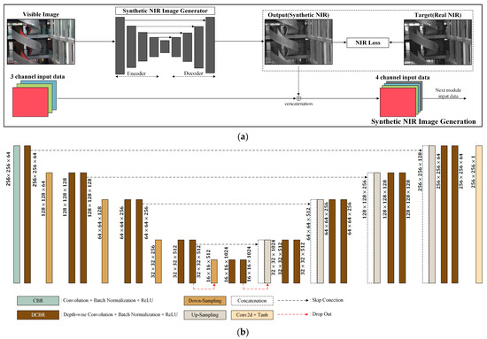
Figure 3.
The training process of the first stage: (a) Flow chart of synthetic NIR image generation; (b) Architecture of the synthetic NIR image generator.
As shown in Figure 3a, the first stage of the proposed method involves generating a synthetic NIR image from an input visible image composed of three RGB channels. The synthetic NIR image generator processes the input and produces a synthetic NIR image, with the difference between the synthetic NIR and the target real NIR image computed using the Mean Square Error (MSE) loss function, given by Equation (7). The generated synthetic NIR image is then concatenated with the input visible image, forming a four-channel input tensor that serves as input for the second stage of training. Figure 3b illustrates the architecture of the synthetic NIR image generator, which is based on a U-Net structure but incorporates Depth-wise Separable Convolution (DS convolution) to reduce the number of parameters and improve computational efficiency. The standard convolution layer generates each output channel by performing convolution operations across all input channels. In contrast, the DS convolution layer applies spatial convolution independently to each input channel, followed by a 1 × 1 pointwise convolution to capture inter-channel dependencies, thereby significantly reducing both computational cost and the number of parameters [36]. The following equations compare the computational processes of standard convolution and DS convolution when applied to a single layer, and present the corresponding FLOPs required for a U-Net architecture based on each method. Equation (3) provides the calculation of MACs for a single layer using standard convolution, while Equation (4) describes the computation involved in a DS convolution layer, which consists of both depth-wise and pointwise convolutions. Equations (5) and (6) present the total FLOPs required for the U-Net architecture when standard convolution and DS convolution are used, respectively.
The variables and represent the height and width of the input image, respectively. The kernel size is denoted by , while and indicate the number of input and output channels. DS convolution reduces the number of parameters and the computational cost by applying spatial convolution independently to each input channel, followed by a pointwise convolution to integrate inter-channel information. In the case of a U-Net architecture with an input image size of and a kernel size of 3, the total number of MACs and FLOPs required by standard convolution is approximately 6.05 billion and 12.1 billion, respectively. When all convolutional layers are replaced with DS convolution, the MACs and FLOPs are reduced to approximately 3.05 billion and 6.1 billion, respectively.
The network consists of two primary building blocks. The CBR block consists of a 3 × 3 convolution layer followed by batch normalization and the ReLU activation function. The DCBR block employs DS convolution and includes 1 × 1 and 3 × 3 convolution layers, batch normalization, and the ReLU activation function. Down-sampling is performed using MaxPooling to reduce feature map size, while up-sampling is achieved through ConvTranspose operations to restore resolution. To prevent overfitting, dropout is applied at the end of the encoder and the beginning of the decoder. The final layer employs the tanh activation function, which ensures stable learning due to its symmetric properties around zero and mitigates the vanishing gradient problem more effectively than the sigmoid function.
where and represent the height and width of the image, respectively; denotes the pixel intensity of the real NIR image at the position ; and denotes the pixel intensity of the generated NIR image at the same position.
The tone distribution of NIR images more directly reflects lighting intensity and material reflectance characteristics compared to conventional visible images. In particular, NIR images tend to preserve structural details more effectively in organic tissues such as vegetation and human skin. This distributional property of NIR images can serve as a useful auxiliary cue for estimating missing HDR information in tone-compressed LDR images. In visible images, overexposure in bright regions often results in the loss of fine details, while underexposed dark regions may exhibit a complete absence of structural content. In contrast, NIR images tend to retain structural information more robustly even under such extreme illumination conditions.
Figure 4 visually illustrates the differences in tone distribution between a visible image and a corresponding NIR image. In Figure 4a, the visible image shows that structural details such as trees and clouds within the red box are barely discernible, whereas in Figure 4b, the NIR image demonstrates that the same regions retain comparatively clear structural details. These distributional differences are further substantiated by the histograms shown at the bottom. As illustrated in Figure 4c, the histogram of the visible image reveals that most pixel intensities are clustered near 0 or 255, indicating a loss of detail due to extreme brightness or darkness. In contrast, the histogram of the NIR image in Figure 4d exhibits a more balanced distribution, with pixel values spanning approximately from 30 to 200. This implies that the NIR image preserves a wider range of tonal details. Such characteristics of NIR tone distribution provide a meaningful rationale for mimicking NIR characteristics to support and restore HDR information that is otherwise lost in LDR visible images.
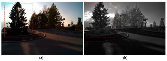
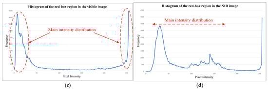
Figure 4.
Comparisons of tone distributions between visible and NIR images with local histogram analysis: (a) Visible image; (b) NIR Image; (c) Histogram of the red box region in the visible image; (d) Histogram of the red box region in the NIR image.
The similarity between the generated synthetic NIR and real NIR images was evaluated using MSE. Figure 5 provides a visual comparison of the RGB image, the real NIR image, and the synthetic NIR image generated during first-stage training. The synthetic NIR image successfully preserves structural information that is absent in the RGB image and aligns with the target real NIR image in key regions. In particular, specific areas in Figure 5 demonstrate how the synthetic NIR image follows the boundaries of the real NIR image, effectively capturing important structural details.
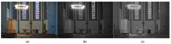
Figure 5.
Results of synthetic NIR images: (a) Input visible image; (b) Real NIR image; (c) Synthetic NIR image.
3.2. HDR Image Generation
In the second stage, the generated synthetic NIR image from the first stage is synthesized with the input visible image. To achieve this, an Autoencoder (AE) structure comprising an encoder and decoder is employed. The encoder extracts meaningful features from the input image, while the decoder reconstructs the image from the latent space based on the extracted features. This study focuses primarily on the encoder’s function, as it plays a crucial role in feature extraction, rather than the performance of the decoder.
Figure 6 provides an overview of the HDR image generation process. Initially, the Visible image and the synthetic NIR image generated in the first stage are concatenated and used as input data. This combined tensor is fed into the HDR image generator, where the resulting HDR image is compared against the target HDR image to compute the loss. The loss is quantified using three primary functions: VGG Loss, SSIM Loss, and MSE Loss. Beyond direct comparison with the target image, a discriminator is incorporated to differentiate between the generated and target images, facilitating the calculation of adversarial loss. Additionally, IQA metrics, NIQE, and BRISQUE are introduced to guide the model toward generating high-quality outputs through supervised learning. The overall learning process is designed to optimize three key loss components. (1) Loss derived from direct comparison with the target image. (2) Adversarial loss obtained via the discriminator. (3) Additional losses aimed at minimizing NIQE and BRISQUE values to enhance output quality. The formulations of these loss functions are as follows:
where represents the total number of pixels, denotes the pixel intensity of the generated output image at the index , and corresponds to the pixel intensity of the target image at the same index. This function measures the average squared difference between the output and target images, ensuring that the generated image closely approximates the target by minimizing reconstruction errors.
where and represent the mean intensities of images and , respectively; and denote their variances; and corresponds to the covariance between them. The constants and stabilize the division to prevent numerical instabilities. Minimizing improves the structural similarity between the generated and target images, preserving perceptual quality.
where represents the VGG loss, which measures perceptual similarity between the output image and the target image . The function represents feature maps extracted from the -th layer of a pre-trained VGG network, and is the weight assigned to that layer. This loss is computed as the weighted sum of the squared -norm differences between the feature representations of and , ensuring that high-level perceptual characteristics are preserved in the generated images.
where represents the discriminator loss, which consists of two terms. The first term, , encourages the discriminator to correctly classify real images by maximizing the likelihood of being close to 1. The second term, , ensures the discriminator correctly identifies generated images as synthetic by maximizing the likelihood of being close to 0. By minimizing , the discriminator improves its ability to distinguish between real and synthetic images. The adversarial loss, , enhances the realism of the generated image. Here, represents the discriminator’s predicted probability that the generated image is real. The expectation is taken over the distribution of generated images, ensuring the generator produces outputs that are increasingly indistinguishable from real images. By minimizing , the generator is trained to create images that align more closely with the real data distribution.
where represents the total generator loss, calculated as a weighted sum of multiple loss components. The first term, , accounts for the mean squared error loss, with as its weight. The second term, , corresponds to the structural similarity index loss, weighted by . The third term, , represents the VGG-based perceptual loss, controlled by . Additionally, contributes the adversarial loss, while and account for the BRISQUE and NIQE image quality losses, respectively. The total loss function balances these components to ensure the generated images maintain perceptual quality and high fidelity across different evaluation metrics.
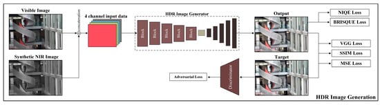
Figure 6.
The training process of the second stage.
In the encoder-decoder framework, the encoder extracts meaningful feature representations from the input, while the decoder reconstructs the image while preserving spatial details. To maximize feature extraction from the Visible image and the synthetic NIR image, an Encoder Block comprising E-ELAN and diff-CBAM is incorporated. Figure 7a illustrates the HDR image generator architecture, where the encoder consists of five Encoder Blocks, and the decoder includes layers integrated with diff-CBAM. Figure 7b presents the discriminator architecture, which consists of five standard convolutional layers. Figure 7c depicts the Encoder Block structure, which is composed of an input layer with a convolutional layer and a diff-CBAM, followed by E-ELAN for feature extraction. E-ELAN is designed to enhance feature diversity through three cardinality operations: Expansion, Shuffle, and Merge. These mechanisms improve gradient flow, feature representation, and computational efficiency within the Encoder Block. Additionally, to achieve a lightweight model while reducing computational complexity, the standard convolutional layers in the Encoder block are replaced with DS Convolution layers. This design is applied in the same manner as the previously mentioned modules, achieving both model lightweight and reduced computational load while maintaining transformation performance.
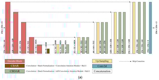
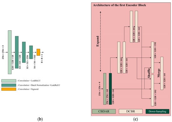
Figure 7.
Architecture of the generator: (a) HDR image generator architecture; (b) discriminator architecture; and (c) encoder block architecture.
Figure 8 illustrates both the architecture of the proposed diff-CBAM and an example that visualizes the difference between input modalities. Figure 8a shows the structure of diff-CBAM within the overall network. CBAM is a computationally efficient attention module for CNN-based architectures that enhances feature learning by generating channel and spatial attention maps. The Channel Attention Module identifies the most relevant channels, while the Spatial Attention Module determines the important spatial regions. In this study, a Difference Map is additionally introduced to the Channel Attention Module to improve its representation capability beyond the conventional CBAM structure.
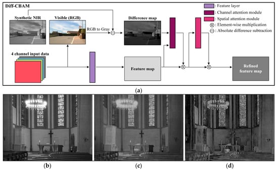
Figure 8.
Structure of the Diff-CBAM and visualization of the difference map: (a) Architecture of Diff-CBAM; (b) Gray image; (c) Synthetic NIR image; (d) Difference map.
Figure 8b–d shows the grayscale visible image, the synthetic NIR image generated from the previous module, and the resulting Difference Map, respectively. The Difference Map clearly highlights distinctive responses between the two modalities in semantically meaningful regions, such as the chandelier, stained-glass windows, and the altar area. These differences originate from variations in material properties, lighting reflections, and spectral responses, which are difficult to capture when simply concatenating the visible and NIR images along the channel dimension.
While the conventional Channel Attention Module in CBAM learns channel-wise importance based on internal feature statistics, it does not incorporate external information regarding cross-domain differences. In this work, the Difference Map is provided as additional input to the Channel Attention Module, guiding the network to focus on channels that effectively capture the discrepancies between the visible and NIR domains. This enables the selection of more structurally and semantically meaningful channels, ultimately contributing to improved HDR reconstruction performance. The effectiveness of this modification is further validated through ablation studies presented in the simulation experiments.
4. Simulation and Results
A total of 984 images were used for training, sourced from the SSMID, TAS-NIR, and RGB-NIR datasets provided by EPFL. These datasets can be downloaded from the following links: (https://github.com/xavysp/ssmid-dataset, https://mucar3.de/iros2022-ppniv-tas-nir/, https://www.epfl.ch/labs/ivrl/research/downloads/rgb-nir-scene-dataset/) (accessed on 16 August 2025) [37,38,39]. The datasets differ in resolution and characteristics due to variations in camera parameters and system-related factors. These differences were intentionally introduced to enhance the model’s generalization performance by combining data from different sources for training.
The proposed model consists of a two-stage inference pipeline. In the first stage, a synthetic NIR image is generated from the input RGB image. For input images with a resolution of 256 × 256, the average inference time in this stage is measured to be 0.0102 s, with GPU memory usage of approximately 445.84 MB and system memory usage of about 690.57 MB. In the second stage, the synthetic NIR image is fused with the original RGB input to generate a final HDR-reflected output. This stage requires an average inference time of 0.0215 s, with GPU and system memory usage of approximately 6008 MB and 790.62 MB, respectively. These measurements were obtained using an NVIDIA RTX 4090 GPU (16,384 CUDA cores, 82.6 TFLOPs). Considering the computational gap between the RTX 4090 and the Google Cloud Platform’s NVIDIA T4 GPU (2560 CUDA cores, 8.1 TFLOPs, priced at $0.35/h), a conservative scaling factor of ×10 was applied to estimate cloud deployment performance. Under this adjustment, the first stage is estimated to require approximately 102 s for processing 1000 images, incurring a cost of around $0.0099. The second stage is estimated to take 215 s for the same batch, with a corresponding cost of approximately $0.0209. Consequently, the total cost for processing 1000 images through both stages is only about $0.0308, indicating the model’s high cost-efficiency and scalability in cloud-based deployment scenarios.
Section 4 consists of two primary experiments. Section 4.1 presents an ablation study, where the effectiveness of each component in the proposed method is evaluated by sequentially removing individual features. Section 4.2 provides a performance comparison, demonstrating the superiority of the proposed method through both qualitative and quantitative analyses, in comparison to existing HDR methods.
4.1. Ablation Experiments
To assess the performance of each module, experiments were conducted by systematically removing individual components. The proposed method is divided into four stages, with the components included in each stage summarized in Table 1.

Table 1.
Configurations for each case in the ablation study.
- Case 1: consists of a DSU-Net for generating synthetic NIR images and an Autoencoder-based HDR image generator that synthesizes synthetic NIR images with Visible images.
- Case 2: adds E-ELAN to the encoder structure of the HDR image generator, enabling an analysis of the impact of E-ELAN by comparing it to Case 1.
- Case 3: introduces Diff-CBAM to both the encoder and decoder of the HDR image generator, facilitating an evaluation of the effect of Diff-CBAM by comparing it to Case 2.
- Case 4: includes Perceptual Quality Optimization, which uses BRISQUE and NIQE metrics to guide the training process. By comparing Case 4 with Case 3, the impact of this training strategy on performance can be assessed.
The effectiveness of each component in the proposed method is validated through an ablation study, in which output images at each stage are compared. Figure 9 and Figure 10 show a comparative analysis at each stage of the proposed pipeline. In the red-boxed region of Figure 9, although the earlier stages—namely Figure 9b–d—show overall enhancement in tone and detail, the extremely dark areas, such as the underside of the vehicle, still suffer from detail loss. In contrast, the final stage, Figure 9e, successfully restores details in the lower region while effectively suppressing noise in unrelated areas. Similarly, in Figure 10, while Figure 10b–d exhibit improvements in tone and detail, the details within the red-boxed region are not sufficiently restored. However, the final result clearly enhances those details while maintaining stable noise suppression across the entire image.
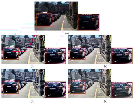
Figure 9.
Qualitative comparison in ablation experiment (highlighted on the lower part of the vehicle): (a) input; (b) case 1; (c) case 2; (d) case 3; (e) case 4.
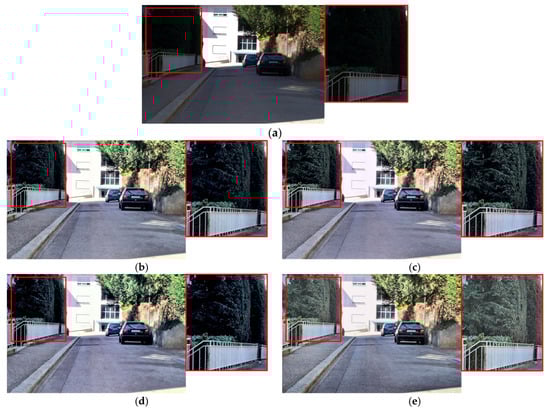
Figure 10.
Qualitative comparison in ablation experiment (highlighted on the trees): (a) input; (b) case 1; (c) case 2; (d) case 3; (e) case 4.
4.2. Performance Comparisons
To validate the performance of the proposed method, both qualitative and quantitative evaluations were conducted. The quantitative evaluation utilized no-reference IQA metrics, comparing the proposed method with existing HDR techniques. Quality scores were calculated using these metrics, and the average values were summarized in a table for comparison. Additionally, a qualitative evaluation was performed to visually demonstrate the advantages of the proposed method.
In the quantitative evaluation, the average quality score was measured for a total of 76 images. The dataset used for this evaluation, the MIT Adobe 5K dataset, differs from the training datasets, which was intentional to test the generalization performance of the model (https://data.csail.mit.edu/graphics/fivek/) (accessed on 16 August 2025) [40]. Furthermore, the visual evaluation involved randomly selecting samples not included in the training data from each dataset. Section 4.2.1 presents the qualitative evaluation results, while Section 4.2.2 provides a detailed description of the quantitative evaluation results.
4.2.1. Qualitative Evaluation
For both qualitative and quantitative evaluations, the comparison targets range from conventional image enhancement algorithms to recent CNN-based methods that estimate HDR information from a single LDR image and present the results visually through tone mapping. HDRUNet is a learning-based model with a spatially dynamic encoder–decoder architecture that performs HDR reconstruction from a single LDR image, including noise removal and dequantization [41]. ExpandNet employs a multi-scale CNN architecture to recover information lost due to quantization, clipping, and tone mapping from a single LDR input image, thereby converting it into an HDR image [42]. LHDR adopts a lightweight DNN architecture and degradation modeling to reconstruct HDR images from degraded LDR inputs [43]. All three methods restore HDR information from LDR images, and the comparison is conducted using the tone-mapped results of the reconstructed HDR images based on the original LDR inputs.
In Figure 11, subfigure (a) depicts the original input, while subfigures (b)–(g) represent the results of existing HDR reconstruction methods. These conventional approaches tend to produce globally brightened outputs, but at the cost of texture fidelity and chromatic richness, often accompanied by noticeable noise artifacts in both low- and mid-luminance regions. In contrast, the proposed method, shown in subfigure (h), exhibits superior chromatic fidelity with vivid yet natural color reproduction, fine detail preservation across intricate structures such as foliage, and effective noise suppression. This combination results in a perceptually more pleasing and visually faithful reconstruction compared to competing methods.
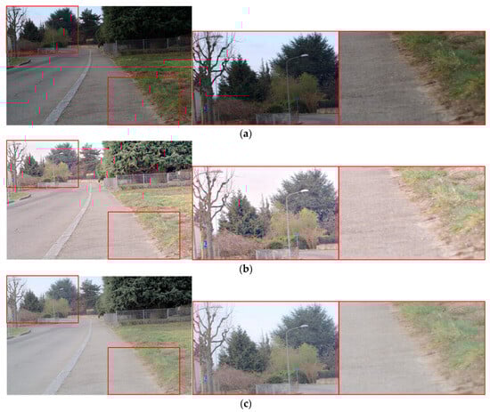
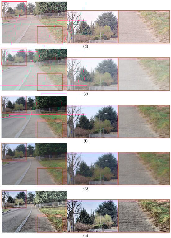
Figure 11.
Qualitative comparison with other methods in outdoor scenes (highlighted on the road boundaries and forest region): (a) original; (b) icam06; (c) L1L0; (d) Kwon; (e) HDRUNet; (f) ExpandNet; (g) LHDR; (h) proposed.
Figure 12 depicts a scene comprising an interior wall on the left, a high-luminance window saturated by intense light in the upper-right, and orange chairs located in the lower-right. Existing methods tend to exaggerate the luminance contrast between the interior and exterior regions, or suffer from detail loss around the bright window area due to excessive outdoor brightness and low indoor illumination. In contrast, the proposed method achieves a clear luminance enhancement in the interior while suppressing excessive brightness in the exterior, thereby maintaining a stable photometric balance between the two regions. Moreover, the proposed method exhibits superior fine-structure preservation in the texture of the wall and the orange chairs, while ensuring smooth tonal transitions without detail loss around the high-luminance window. As a result, the output presents improved visual harmony and spatial depth perception compared with other methods.
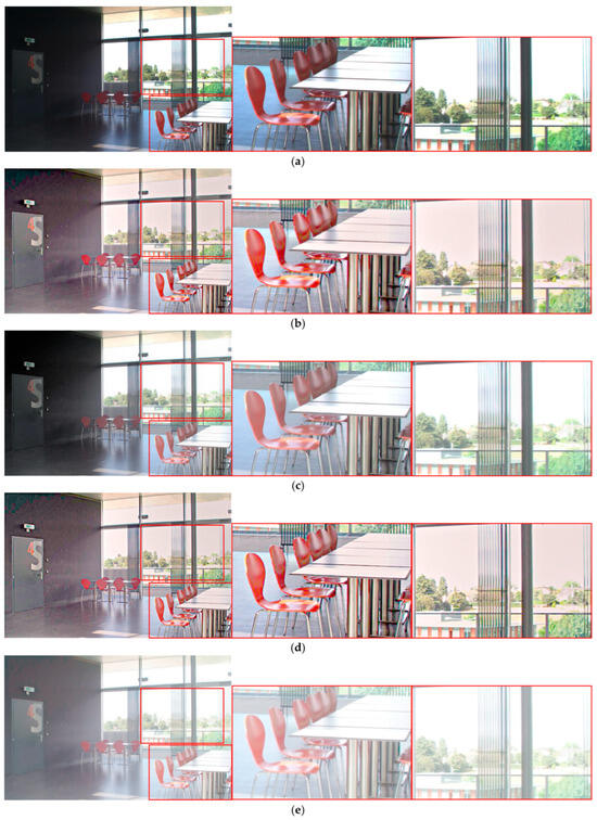
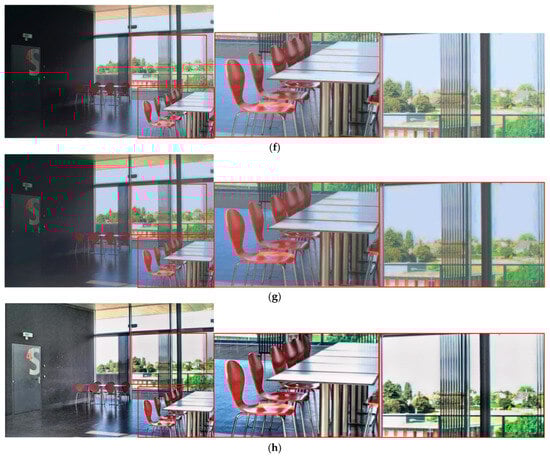
Figure 12.
Qualitative comparison with other methods in indoor scenes (highlighted on the windows regions, chairs, and tables): (a) original; (b) icam06; (c) L1L0; (d) Kwon; (e) HDRUNet; (f) ExpandNet; (g) LHDR; (h) proposed.
Figure 13 depicts a ceiling fitted with white-framed windows, a transparent glass wall with text on the right, and a yellow-and-blue structural element on the left. Existing methods generally increase overall luminance to achieve a tone-up effect; however, some exhibit noticeable color desaturation and a loss of detail in shaded or recessed areas. In contrast, the proposed method preserves vivid color reproduction without desaturation while effectively retaining fine textures in dark corners and complex structural regions. This results in enhanced visual contrast between the foreground and background, thereby improving the overall depth perception and aesthetic quality of the scene.
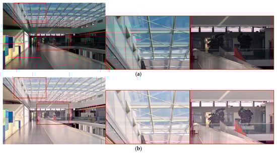
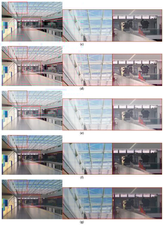
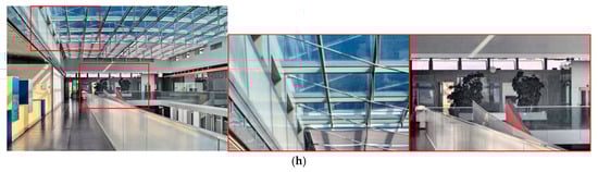
Figure 13.
Qualitative comparison with other methods in indoor scenes (highlighted on the ceiling window grids and interior building details): (a) original; (b) icam06; (c) L1L0; (d) Kwon; (e) HDRUNet; (f) ExpandNet; (g) LHDR; (h) proposed.
Figure 14 shows the interior of a cathedral, with a podium located at the lower left. Other methods brighten the dark podium area but introduce noise, and the chromaticity of the stained-glass windows decreases as luminance increases. The proposed method distinguishes the podium from the dark background while suppressing noise and preserving the chromaticity of the stained-glass windows.
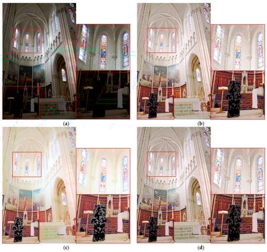
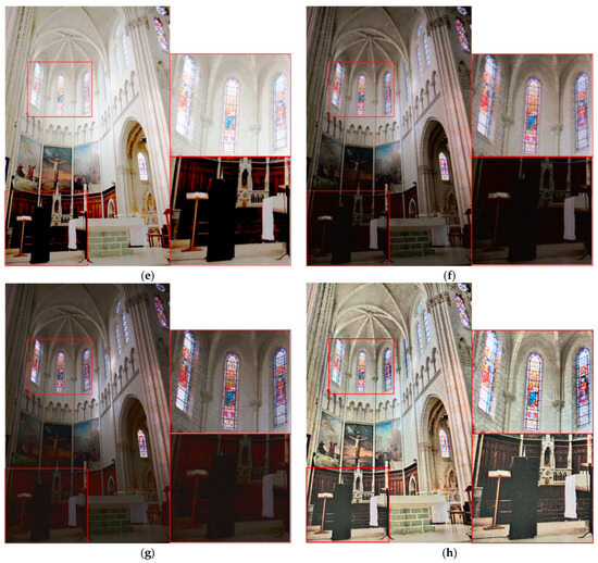
Figure 14.
Qualitative comparison with other methods in indoor scenes (highlighted on the pulpit and the stained-glass windows): (a) original; (b) icam06; (c) L1L0; (d) Kwon; (e) HDRUNet; (f) ExpandNet; (g) LHDR; (h) proposed.
Figure 15 depicts the front façade of a brick cathedral, with a similarly constructed building in the background. In the foreground, a woman in a white shirt and an individual dressed in a black top carrying a black bag are present. In the original image, the faces of both individuals are entirely unrecognizable; however, the proposed method renders them with sufficient clarity to allow identification. While other methods achieve partial improvement in this regard, the proposed method offers the highest level of recognizability, delivering superior detail preservation and overall visual sharpness.
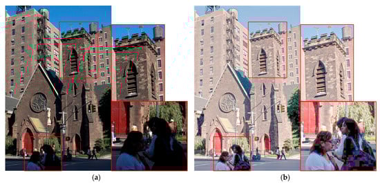
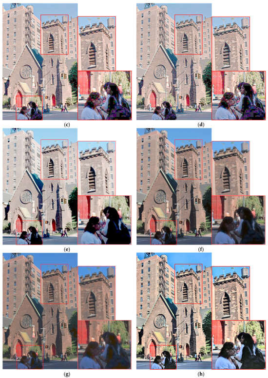
Figure 15.
Qualitative comparison with other methods in outdoor scenes (highlighted on the brick building façade and the pedestrians): (a) original; (b) icam06; (c) L1L0; (d) Kwon; (e) HDRUNet; (f) ExpandNet; (g) LHDR; (h) proposed.
Figure 16 depicts a scene captured from indoors through a window, simultaneously showing both the interior and the exterior. The interior appears very dark, while the exterior is bright. In the original image, the chair beneath the window is barely discernible, and the comparative methods render the chair only faintly while failing to clearly define the boundary between the window and the interior. In contrast, the proposed method distinctly reveals both the chair and the interior–exterior boundary. Although this comes at the cost of a slightly higher level of noise compared to other methods, it achieves superior detail reproduction, resulting in a more realistic and visually informative representation.
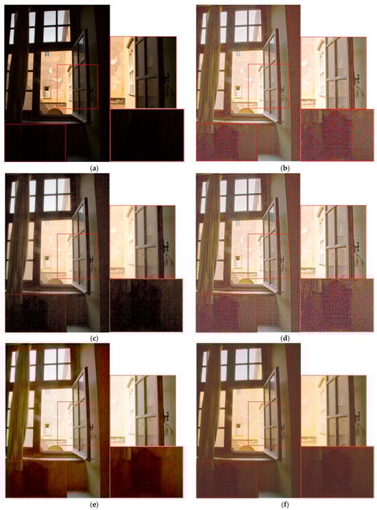
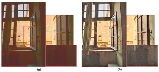
Figure 16.
Qualitative comparison with other methods in indoor scenes (highlighted on the indoor chairs and the window boundaries between the interior and exterior) (a) original; (b) icam06; (c) L1L0; (d) Kwon; (e) HDRUNet; (f) ExpandNet; (g) LHDR; (h) proposed.
4.2.2. Quantitative Evaluation
For the quantitative evaluation, 76 samples were selected from the MIT Adobe 5K dataset, which differs from the training datasets, thereby testing the generalization performance of the proposed method. The experiments on this independent dataset help demonstrate the method’s robustness beyond HDR performance within the same dataset.
For quantitative image quality assessment, IQA is used to evaluate image degradation caused by processes like compression, transmission, and restoration. IQA methods are categorized into Full-Reference IQA (FR-IQA) and No-Reference IQA (NR-IQA), with the primary distinction being whether a reference image is available for evaluation.
The metrics employed in this study are all objective, no-reference image quality indicators. BRISQUE is a no-reference model based on natural scene statistics, using locally normalized luminance coefficients to quantify the loss of naturalness in images [44]. NRPQA is a no-reference algorithm for JPEG compressed images, based on subjective quality evaluation experiments [45]. SSEQ utilizes local spatial and spectral entropy features to assess image quality [46]. MANIQA uses a Vision Transformer to extract image features and introduces a patch-based weighted quality prediction structure [47]. CNNIQA integrates feature learning and regression into a single optimization process for effective quality prediction [48].
Table 2 and Figure 17 present the average scores for the 76 images across each metric. In the lower arrows (↓), smaller values indicate better quality, as shown in Figure 18, Figure 19 and Figure 20, where smaller circles correspond to higher quality. On the other hand, in the case of the upward arrows (↑), larger values indicate better quality, and in Figure 21 and Figure 22, larger circle represent better quality. The proposed method demonstrates overall superior performance compared to other approaches, with only a few cases ranking second or third. In particular, when compared with the ExpandNet and LHDR methods, it shows a marginal disadvantage in the NRPQA and MANIQA metrics, yet achieves a significant advantage in the SSEQ and BRISQUE metrics. These results substantiate the competitiveness of the proposed method across a wide range of image quality evaluation indicators.
Table 2.
Comparison of scores by metric (↓: lower is better quality, ↑: higher is better quality).
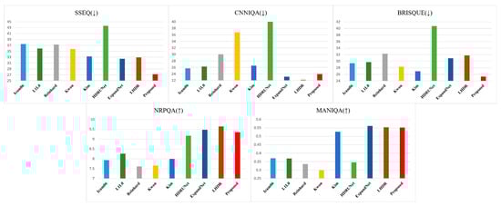
Figure 17.
Average scores for 76 images (↓: lower is better quality, ↑: higher is better quality).
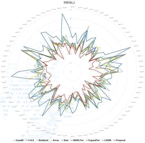
Figure 18.
SSEQ score distribution for 76 images.
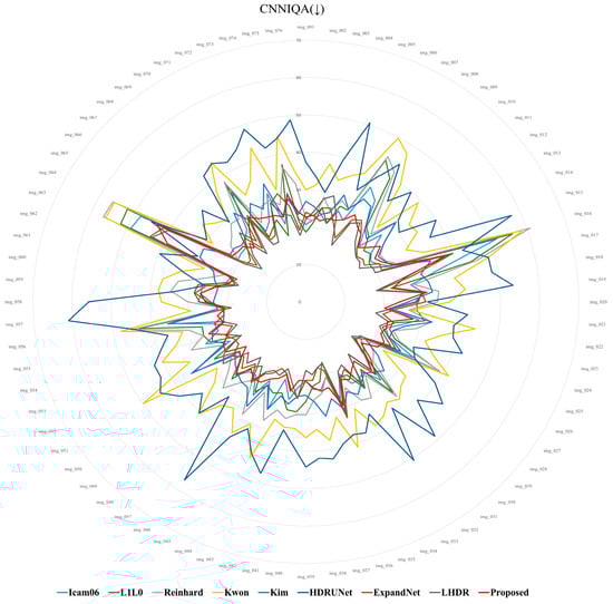
Figure 19.
CNNIQA score distribution for 76 images.
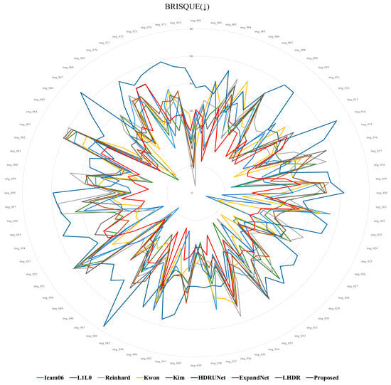
Figure 20.
BRISQUE score distribution for 76 images.
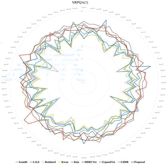
Figure 21.
NRPQA score distribution for 76 images.
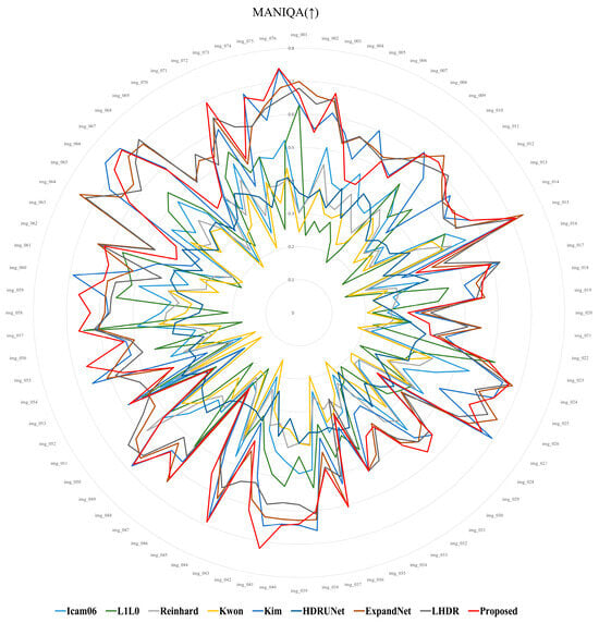
Figure 22.
MANIQA score distribution for 76 images.
5. Conclusions
In this study, we proposed a novel method for generating synthetic NIR images from a single LDR image and fusing them with the original LDR image to produce an extended dynamic range image. The synthetic NIR image is generated using a lightweight U-Net architecture, where the LDR image is first transformed into a feature map in the encoder and subsequently decoded to reflect NIR characteristics. The generated synthetic NIR image and the original LDR image are then combined into a 4-channel input and processed through a second fusion module, separate from the initial U-Net, to generate an HDR image with an extended dynamic range.
The proposed method addresses the need for more refined feature extraction compared to single-image processing by introducing an enhanced encoder architecture incorporating group-based techniques such as Extend, Shuffle, and Merge, along with a modified attention module, diff-CBAM. In particular, a Difference Map emphasizing the contrast between the LDR and synthetic NIR images was introduced as an additional input to further improve performance. To preserve high-frequency details and generate more natural results, a discriminator was employed, and NR-IQA metrics such as BRISQUE and NIQE were integrated into the loss function to enhance naturalness. The effectiveness of the proposed model was validated through ablation studies and comparative experiments with existing HDR generation methods. Quantitative evaluations using various NR-IQA metrics, including SSEQ, BRISQUE, MANIQA, CNNIQA, and NRIQA, confirmed that the proposed model outperforms prior methods in distortion, naturalness, and overall image quality.
Although the enhanced encoder architecture facilitated more refined feature learning, the latent representation occasionally converged to a limited form, causing the decoder to replicate the input directly. This behavior risks reducing the model’s generalization capability, especially when handling diverse input distributions. To address this limitation, future work will focus on incorporating probabilistic representations within the latent space by employing advanced HDR generation techniques such as Variational Autoencoders (VAE) or Vector Quantization-VAE (VQ-VAE), which jointly improve representation diversity and reconstruction quality.
Author Contributions
Conceptualization, S.H.L. (Sung Hak Lee); methodology, S.H.L. (Seung Hwan Lee) and S.H.L. (Sung Hak Lee); software, S.H.L. (Seung Hwan Lee); validation, S.H.L. (Seung Hwan Lee) and S.H.L. (Sung Hak Lee); formal analysis, S.H.L. (Seung Hwan Lee) and S.H.L. (Sung Hak Lee); investigation, S.H.L. (Seung Hwan Lee) and S.H.L. (Sung Hak Lee); resources, S.H.L. (Seung Hwan Lee) and S.H.L. (Sung Hak Lee); data curation, S.H.L. (Seung Hwan Lee) and S.H.L. (Sung Hak Lee); writing—original draft preparation, S.H.L. (Seung Hwan Lee); writing—review and editing, S.H.L. (Sung Hak Lee); visualization, S.H.L. (Seung Hwan Lee); supervision, S.H.L. (Sung Hak Lee); project administration, S.H.L. (Sung Hak Lee); funding acquisition, S.H.L. (Sung Hak Lee). All authors have read and agreed to the published version of the manuscript.
Funding
This research was supported by Korea Creative Content Agency (KOCCA) grant funded by the Ministry of Culture, Sports and Tourism (MCST) in 2024 (Project Name: Development of optical technology and sharing platform technology to acquire digital cultural heritage for high quality restoration of composite materials cultural heritage, Project Number: RS-2024-00442410, Contribution Rate: 50%) and the Institute of Information & Communications Technology Planning & Evaluation (IITP)-Innovative Human Resource Development for Local Intellectualization program grant funded by the Korea government (MSIT) (IITP-2025-RS-2022-00156389, 50%).
Data Availability Statement
TAS-NIR Dataset: https://mucar3.de/iros2022-ppniv-tas-nir/ [37]. SSMID Dataset: https://github.com/xavysp/ssmid-dataset [38]. RGB–NIR Scene Dataset (EPFL): https://www.epfl.ch/labs/ivrl/research/downloads/rgb-nir-scene-dataset/ [39]. MIT Adobe 5K Dataset: https://data.csail.mit.edu/graphics/fivek/ [40]. All datasets are made freely available to academic and non-academic entities for non-commercial purposes.
Conflicts of Interest
The authors declare no conflict of interest.
References
- Jinno, T.; Okuda, M. Multiple Exposure Fusion for High Dynamic Range Image Acquisition. IEEE Trans. Image Process. 2012, 21, 358–365. [Google Scholar] [CrossRef]
- Simons, R.H. Comment 2 on ‘Evaluation of High Dynamic Range Photography as a Luminance Data Acquisition System’ by M.N. Inanici. Light. Res. Technol. 2006, 38, 135. [Google Scholar] [CrossRef]
- Banterle, F.; Ledda, P.; Debattista, K.; Chalmers, A. Inverse Tone Mapping. In Proceedings of the 4th International Conference on Computer Graphics and Interactive Techniques in Australasia and Southeast Asia (GRAPHITE 2006), Kuala Lumpur, Malaysia, 29 November–2 December 2006; ACM: New York, NY, USA, 2006; pp. 349–356. [Google Scholar] [CrossRef]
- Eilertsen, G.; Kronander, J.; Denes, G.; Mantiuk, R.K.; Unger, J. HDR Image Reconstruction from a Single Exposure Using Deep CNNs. ACM Trans. Graph. 2017, 36, 178. [Google Scholar] [CrossRef]
- García-Rey, R.M.; García-Olmo, J.; De Pedro, E.; Quiles-Zafra, R.; Luque de Castro, M.D. Prediction of Texture and Colour of Dry-Cured Ham by Visible and near Infrared Spectroscopy Using a Fiber Optic Probe. Meat Sci. 2005, 70, 357–363. [Google Scholar] [CrossRef]
- Liu, Y.; Lyon, B.G.; Windham, W.R.; Realini, C.E.; Pringle, T.D.; Duckett, S. Prediction of Color, Texture, and Sensory Characteristics of Beef Steaks by Visible and near Infrared Reflectance Spectroscopy—A Feasibility Study. Meat Sci. 2003, 65, 1107–1115. [Google Scholar] [CrossRef]
- Liu, Y.; Chen, Y.; Ozaki, Y. Two-Dimensional Visible/Near-Infrared Correlation Spectroscopy. Appl. Spectrosc. 2000, 54, 901–908. [Google Scholar] [CrossRef]
- Chudnovsky, A.; Ben-Dor, E. Application of Visible, Near-Infrared, and Short-Wave Infrared (400–2500 nm) Reflectance Spectroscopy in Quantitatively Assessing Settled Dust in the Indoor Environment: Case Study in Dwellings and Office Environments. Sci. Total Environ. 2008, 393, 198–213. [Google Scholar] [CrossRef] [PubMed]
- Yang, T.; Li, Y.; Ruichek, Y.; Yan, Z. Performance Modeling a Near-Infrared ToF LiDAR Under Fog: A Data-Driven Approach. IEEE Trans. Intell. Transp. Syst. 2022, 23, 11227–11236. [Google Scholar] [CrossRef]
- Kil, T.; Cho, N.I. Image Fusion Using RGB and Near Infrared Image. J. Broadcast Eng. 2016, 21, 515–524. [Google Scholar] [CrossRef]
- Lee, J.; Oh, G.; Jeon, B. Perceptual Image Fusion Technique of RGB and NIR Images. In Proceedings of the 34th International Technical Conference on Circuits/Systems, Computers and Communications (ITC-CSCC 2019), JeJu, Republic of Korea, 23–26 June 2019; IEEE: New York, NY, USA, 2019; pp. 127–130. [Google Scholar] [CrossRef]
- Soundari, V.D.; Rabin, G.; Rishiyugan, S.; Pravinkumar, P. Image Processing for LDR to HDR Image Conversion Using Deep Learning. In Proceedings of the 5th International Conference on Inventive Research in Computing Applications (ICIRCA 2023), Coimbatore, India, 5–7 July 2023; IEEE: New York, NY, USA, 2023; pp. 146–150. [Google Scholar] [CrossRef]
- Raipurkar, P.; Pal, R.; Raman, S. HDR-CGAN: Single LDR to HDR Image Translation Using Conditional GAN. In Proceedings of the 2021 ACM International Conference on Multimedia Asia (MMAsia ’21), Gold Coast, Australia, 1–3 December 2021; ACM: New York, NY, USA, 2021. [Google Scholar] [CrossRef]
- Bhatt, D.; Patel, C.; Talsania, H.; Patel, J.; Vaghela, R.; Pandya, S.; Modi, K.; Ghayvat, H. CNN Variants for Computer Vision: History, Architecture, Application, Challenges and Future Scope. Electronics 2021, 10, 2470. [Google Scholar] [CrossRef]
- Woo, S.; Park, J.; Lee, J.; Kweon, I.S. CBAM: Convolutional Block Attention Module. In Proceedings of the 15th European Conference on Computer Vision (ECCV 2018), Munich, Germany, 8–14 September 2018; Springer: Cham, Switzerland, 2018; pp. 3–19. [Google Scholar] [CrossRef]
- Zhang, H.; Goodfellow, I.; Metaxas, D.; Odena, A. Self-Attention Generative Adversarial Networks. In Proceedings of the 36th International Conference on Machine Learning (ICML 2019), Long Beach, CA, USA, 9–15 June 2019; PMLR: London, UK, 2019; pp. 7354–7363. [Google Scholar]
- Kwon, H.; Lee, S.; Lee, G.; Sohng, K. Enhanced High Dynamic-Range Image Rendering Using a Surround Map Based on Edge-Adaptive Layer Blurring. IET Comput. Vis. 2016, 10, 689–699. [Google Scholar] [CrossRef]
- Kim, Y.J.; Son, D.M.; Lee, S.H. Retinex Jointed Multiscale CLAHE Model for HDR Image Tone Compression. Mathematics 2024, 12, 1541. [Google Scholar] [CrossRef]
- Kuang, J.; Johnson, G.M.; Fairchild, M.D. ICAM06: A Refined Image Appearance Model for HDR Image Rendering. J. Vis. Commun. Image Represent. 2007, 18, 406–414. [Google Scholar] [CrossRef]
- Reinhard, E.; Stark, M.; Shirley, P.; Ferwerda, J. Photographic Tone Reproduction for Digital Images. ACM Trans. Graph. 2002, 21, 267–276. [Google Scholar] [CrossRef]
- Liang, Z.; Xu, J.; Zhang, D.; Cao, Z.; Zhang, L. A Hybrid L1-L0 Layer Decomposition Model for Tone Mapping. In Proceedings of the IEEE Conference on Computer Vision and Pattern Recognition (CVPR 2018), Salt Lake City, UT, USA, 18–23 June 2018; IEEE: New York, NY, USA, 2018; pp. 4758–4766. [Google Scholar] [CrossRef]
- Lee, M.J.; Rhee, C.H.; Lee, C.H. HSVNet: Reconstructing HDR Image from a Single Exposure LDR Image with CNN. Appl. Sci. 2022, 12, 2370. [Google Scholar] [CrossRef]
- An, J.; Lee, S.H.; Kuk, J.G.; Cho, N.I. A Multi-Exposure Image Fusion Algorithm without Ghost Effect. In Proceedings of the IEEE International Conference on Acoustics, Speech and Signal Processing (ICASSP 2011), Prague, Czech Republic, 22–27 May 2011; IEEE: New York, NY, USA, 2011; pp. 1565–1568. [Google Scholar] [CrossRef]
- Merianos, I.; Mitianoudis, N. Multiple-Exposure Image Fusion for HDR Image Synthesis Using Learned Analysis Transformations. J. Imaging 2019, 5, 32. [Google Scholar] [CrossRef]
- Mitianoudis, N.; Stathaki, T. Optimal Contrast Correction for ICA-Based Fusion of Multimodal Images. IEEE Sens. J. 2008, 8, 2016–2026. [Google Scholar] [CrossRef]
- Mertens, T.; Kautz, J.; Van Reeth, F. Exposure Fusion. In Proceedings of the 15th Pacific Conference on Computer Graphics and Applications (PG’07), Maui, HI, USA, 29 October–2 November 2007; IEEE: New York, NY, USA, 2007; pp. 382–390. [Google Scholar] [CrossRef]
- Hu, X.; Shen, L.; Jiang, M.; Ma, R.; An, P. LA-HDR: Light Adaptive HDR Reconstruction Framework for Single LDR Image Considering Varied Light Conditions. IEEE Trans. Multimed. 2023, 25, 4814–4829. [Google Scholar] [CrossRef]
- Son, D.M.; Kwon, H.J.; Lee, S.H. Visible and Near Infrared Image Fusion Using Base Tone Compression and Detail Transform Fusion. In Proceedings of the 2022 International Conference on Electrical, Computer and Energy Technologies (ICECET 2022), Prague, Czech Republic, 20–22 July 2022; IEEE: New York, NY, USA, 2022; pp. 1–6, ISBN 978-8253950725. [Google Scholar]
- Kwon, H.J.; Lee, S.H. Visible and Near-Infrared Image Acquisition and Fusion for Night Surveillance. Chemosensors 2021, 9, 75. [Google Scholar] [CrossRef]
- Simonyan, K.; Zisserman, A. Very Deep Convolutional Networks for Large-Scale Image Recognition. In Proceedings of the 3rd International Conference on Learning Representations (ICLR 2015), San Diego, CA, USA, 7–9 May 2015; pp. 1–14. [Google Scholar]
- He, K.; Zhang, X.; Ren, S.; Sun, J. Deep Residual Learning for Image Recognition. In Proceedings of the IEEE Conference on Computer Vision and Pattern Recognition (CVPR 2016), Las Vegas, NV, USA, 27–30 June 2016; IEEE: New York, NY, USA, 2016; pp. 770–778. [Google Scholar] [CrossRef]
- Zagoruyko, S.; Komodakis, N. Wide Residual Networks. In Proceedings of the British Machine Vision Conference (BMVC 2016), York, UK, 19–22 September 2016; BMVA Press: Durham, UK, 2016; pp. 87.1–87.12. [Google Scholar] [CrossRef]
- Xie, S.; Girshick, R.; Dollár, P.; Tu, Z.; He, K. Aggregated Residual Transformations for Deep Neural Networks. In Proceedings of the IEEE Conference on Computer Vision and Pattern Recognition (CVPR 2017), Honolulu, HI, USA, 21–26 July 2017; IEEE: New York, NY, USA, 2017; pp. 5987–5995. [Google Scholar] [CrossRef]
- Wang, C.-Y.; Bochkovskiy, A.; Liao, H.-Y.M. YOLOv7: Trainable Bag-of-Freebies Sets New State-of-the-Art for Real-Time Object Detectors. arXiv 2022, arXiv:2207.02696. [Google Scholar]
- Wang, C.-Y.; Liao, H.-Y.M.; Yeh, I.-H. Designing Network Design Strategies through Gradient Path Analysis. arXiv 2022, arXiv:2211.04800. [Google Scholar] [CrossRef]
- Chollet, F. Xception: Deep Learning with Depthwise Separable Convolutions. In Proceedings of the IEEE Conference on Computer Vision and Pattern Recognition (CVPR 2017), Honolulu, HI, USA, 21–26 July 2017; IEEE: New York, NY, USA, 2017; pp. 1800–1807. [Google Scholar] [CrossRef]
- Mortimer, P. TAS-NIR: A VIS + NIR Dataset for Fine-Grained Semantic Segmentation in Unstructured Outdoor Environments. Data 2023, 8, 72. [Google Scholar] [CrossRef]
- Soria, X.; Sappa, A.D.; Akbarinia, A. Multispectral single-sensor RGB-NIR imaging: New challenges and opportunities. In Proceedings of the 7th International Conference on Image Processing Theory, Tools and Applications (IPTA), Montreal, QC, Canada, 28 November–1 December 2017; pp. 1–6. [Google Scholar] [CrossRef]
- EPFL IVRL. RGB–NIR Scene Dataset. [Online]. Available online: https://www.epfl.ch/labs/ivrl/research/downloads/rgb-nir-scene-dataset/ (accessed on 8 August 2025).
- MIT CSAIL. MIT Adobe 5K Dataset. [Online]. Available online: https://data.csail.mit.edu/graphics/fivek/ (accessed on 8 August 2025).
- Chen, X.; Liu, Y.; Zhang, Z.; Qiao, Y.; Dong, C. HDRUNet: Single Image HDR Reconstruction with Denoising and Dequantization. In Proceedings of the IEEE/CVF Conference on Computer Vision and Pattern Recognition Workshops (CVPRW 2021), Nashville, TN, USA, 19–25 June 2021; IEEE: New York, NY, USA, 2021; pp. 354–363. [Google Scholar] [CrossRef]
- Marnerides, D.; Bashford-Rogers, T.; Hatchett, J.; Debattista, K. ExpandNet: A Deep Convolutional Neural Network for High Dynamic Range Expansion from Low Dynamic Range Content. Comput. Graph. Forum 2018, 37, 37–49. [Google Scholar] [CrossRef]
- Guo, C.; Jiang, X. LHDR: HDR Reconstruction for Legacy Content Using a Lightweight DNN. In Proceedings of the 17th Asian Conference on Computer Vision (ACCV 2022), Macau, China, 4–8 December 2022; pp. 306–322. [Google Scholar] [CrossRef]
- Mittal, A.; Moorthy, A.K.; Bovik, A.C. No-Reference Image Quality Assessment in the Spatial Domain. IEEE Trans. Image Process. 2012, 21, 4695–4708. [Google Scholar] [CrossRef] [PubMed]
- Wang, Z.; Sheikh, H.R.; Bovik, A.C. No-Reference Perceptual Quality Assessment of JPEG Compressed Images. In Proceedings of the IEEE International Conference on Image Processing (ICIP 2002), Rochester, NY, USA, 22–25 September 2002; pp. 477–480. [Google Scholar] [CrossRef]
- Liu, L.; Liu, B.; Huang, H.; Conrad, A. No-Reference Image Quality Assessment Based on Spatial and Spectral Entropies. Signal Process. Image Commun. 2014, 29, 856–863. [Google Scholar] [CrossRef]
- Yang, S.; Wu, T.; Shi, S.; Lao, S.; Gong, Y. MANIQA: Multi-Dimension Attention Network for No-Reference Image Quality Assessment. In Proceedings of the IEEE/CVF Conference on Computer Vision and Pattern Recognition (CVPR 2022), New Orleans, LA, USA, 18–24 June 2022; pp. 1191–1200. [Google Scholar] [CrossRef]
- Kang, L.; Ye, P.; Li, Y.; Doermann, D. Convolutional Neural Networks for No-Reference Image Quality Assessment. In Proceedings of the IEEE Conference on Computer Vision and Pattern Recognition (CVPR 2014), Columbus, OH, USA, 23–28 June 2014; pp. 1733–1740. [Google Scholar] [CrossRef]
Disclaimer/Publisher’s Note: The statements, opinions and data contained in all publications are solely those of the individual author(s) and contributor(s) and not of MDPI and/or the editor(s). MDPI and/or the editor(s) disclaim responsibility for any injury to people or property resulting from any ideas, methods, instructions or products referred to in the content. |
© 2025 by the authors. Licensee MDPI, Basel, Switzerland. This article is an open access article distributed under the terms and conditions of the Creative Commons Attribution (CC BY) license (https://creativecommons.org/licenses/by/4.0/).