Robust Discontinuity Indicators for High-Order Reconstruction of Piecewise Smooth Functions

Abstract

The accurate reconstruction of piecewise continuous functions on meshes is challenging due to potential spurious oscillations—namely the Gibbs phenomenon—especially for high-order methods. This paper introduces the Robust Discontinuity Indicators (RDI) method, a novel technique for constructing discontinuity indicators. These indicators can effectively identify both $C^0$ and $C^1$ discontinuities in a single pass using a new comprehensive theoretical analysis combined with cell-based overshoot–undershoot indicators and node-based oscillation indicators. In addition to detecting discontinuities, these indicator values can also facilitate the construction of adaptive weighting schemes to mitigate the Gibbs phenomenon. Due to its flexibility, RDI can accommodate complex geometries and applies to nonuniform unstructured meshes and general surfaces, broadening its utility. Through experiments, we show that RDI can accurately capture discontinuities while producing fewer false positives than two-pass methods. By providing a more rigorous method for discontinuity detection, RDI has the potential to offer significant improvements in computational simulations and data remapping.

1. Introduction

The detection and accurate resolution of discontinuities in piecewise continuous functions are pivotal in diverse computational applications, including computer-aided design (CAD), computer graphics, and computational fluid dynamics (CFD) [1,2,3]. Inaccuracies in these processes can lead to non-physical oscillations, known as the Gibbs phenomenon [4], which can severely jeopardize the fidelity of results, especially when high-order methods are used.

Sophisticated numerical methods, such as Discontinuous Galerkin (DG) methods [1], Essentially Non-Oscillatory (ENO) schemes [5], and Weighted Essentially Non-Oscillatory (WENO) schemes [6], have been effectively established to address these issues, especially in handling sharp transitions in the context of solving hyperbolic partial differential equations (PDEs). These challenges extend to other domains, such as in the numerical integration of piecewise-smooth (PWS) dynamical systems, where naive regularization can alter the system’s qualitative behavior [7], making accurate event detection essential [8]. The ENO-SR scheme introduced by Harten [9] further incorporates subcell resolution, which improves the accuracy of discontinuity detection by utilizing cell averages to precisely locate discontinuities within a cell, thus preventing the smearing of features like contact discontinuities. Most of these methods focus on identifying and resolving $C^0$ discontinuities, namely discontinuities in function values. Some works, such as [10,11], can also detect and/or resolve $C^1$ discontinuities, namely discontinuities in the gradients of functions, such as in the context of solving Hamilton–Jacobi equations [10]. The latter is even more crucial in remapping and reconstructing piecewise continuous functions than it is in solving PDEs. Recognizing this challenge, we aim to develop a method for detecting and characterizing $C^0$ and $C^1$ discontinuities. This method should apply to nonuniform, unstructured surface meshes and general surfaces, unlike traditional methods limited to structured meshes or 2D planes. In addition, the indicator values in detecting discontinuities should also be useful for constructing adaptive weighting schemes to resolve the Gibbs phenomenon, such as those used in WENO-like schemes [12,13].

This paper details the Robust Discontinuity Indicators (RDI) method, a sophisticated technique that addresses these challenges. This work significantly expands upon our previous research [13], where the analysis was primarily heuristic and testing was limited to uniform spherical meshes. The main contributions of this paper are a more rigorous theoretical foundation and a significant generalization of the method. Specifically, we provide a systematic theoretical analysis, including proofs, that explains the behavior of the indicators and enables the robust detection of both $C^0$ and $C^1$ discontinuities in a single pass. Furthermore, we generalize the method to accommodate complex geometries with sharp features and nonuniform unstructured meshes, which is critical for practical applications [2]. The enhanced scheme also improves robustness for functions with poor scaling characteristics and, importantly, is extended to handle cell-averaged data, a key requirement for finite volume methods not previously addressed. Finally, through extensive numerical verification, we demonstrate that RDI accurately captures discontinuities while producing fewer false positives than comparable two-pass methods. By enhancing the accuracy of discontinuity detection and resolution, the RDI method can facilitate more consistent and reliable simulations, data remapping, and other computational procedures.

The remainder of this paper is organized as follows. Section 2 provides an introductory overview of weighted least squares approximations and the Gibbs phenomenon. Section 3 presents a detailed analysis of overshoots and undershoots near discontinuities, culminating in the derivation of cell-based overshoot–undershoot indicators. Section 4 introduces node-based oscillation indicators and a dual-thresholding strategy and elaborates on their effective implementation in scenarios involving nonuniform meshes and distinct surface features. Section 5 showcases a series of numerical tests and compares RDI with other state-of-the-art approaches to substantiate the robustness of the RDI method. Lastly, Section 6 summarizes the findings and discusses prospective avenues for further exploration.

2. Background and Preliminaries

Weighted least squares (WLS) is a powerful method for data fitting, remapping, reconstruction, and other applications. However, degree-p WLS with $p\ge 2$ can introduce oscillations near discontinuities [13]. Interestingly, these oscillations can also be useful in detecting discontinuities. In this section, we provide an overview of WLS and discuss the phenomenon of oscillations, commonly referred to as the Gibbs phenomenon. This section also introduces Weighted Averaging of Local Fittings (WALF), a technique used later in the construction of our indicators.

2.1. Related Work

Discontinuities often lead to undesired overshoots or undershoots in numerical methods. Specifically, $C^0$ discontinuities, also known as edges [14], jump discontinuities [15,16], or faults [17,18], have a finite jump in function values. These discontinuities tend to cause $\mathcal{O}\left(1\right)$ oscillations that persist with mesh refinement [13]. This phenomenon is referred to as the Gibbs or Gibbs–Wilbraham phenomenon in the context of the Fourier transform [16]. While $C^0$ discontinuities have been extensively studied, less attention has been given to $C^1$ discontinuities, which have a finite jump in the gradients of functions. Nonetheless, $C^1$ discontinuities are still crucial in various applications. For instance, they often represent junctions or intersections of components, such as features or ridge points. The $C^1$ discontinuities may cause mild oscillations in numerical methods [19].

Detecting these discontinuities is essential for the effective resolution of the Gibbs phenomenon in numerical methods. It also has significant implications for various other applications, such as mesh reconstruction [20] and image processing [21]. Several methods have been developed for edge detection, such as the Polynomial Annihilation Edge Detector (PAED) [22,23,24,25] based on the polynomial annihilation (PA) technique, zero-crossing in the second derivatives [26,27,28], and singularity detection and processing with wavelets (SDPW) [29] based on the wavelet transform. The PA technique in [22] focused on a 2D unstructured mesh, approximating the jump function to detect $C^0$ discontinuities. The work in [23] further utilizes PAED on an approximation of the gradient to detect $C^1$ discontinuities. In [25], the work combined the use of PA techniques to detect discontinuities and applied ${\ell }^1$ regularization to mitigate the Gibbs phenomenon in the context of solving hyperbolic PDEs in 1D. Furthermore, work on variably scaled kernels (VSKs) has shown success in interpolating functions with gradient discontinuities by locally adapting the smoothness of the basis functions to the position of the discontinuities [30]. Separately, recent work has developed methods for polynomial interpolation using mapped bases while avoiding resampling, addressing the Gibbs phenomenon [31]. Unlike these previous works, our method is based on weighted-least squares and can detect both $C^0$ and $C^1$ discontinuities in a single pass without explicitly estimating derivatives. In addition, our method can be applied to general surfaces and nonuniform meshes, which are not addressed in the PA technique. In Section 5.2, we will compare our method with PAED [22,23] and demonstrate that our method tends to produce fewer false positives. It is also worth noting that for general surfaces, we cannot easily transform the problem into 1D problems or apply a Fourier transform, and many existing methods (such as the 1D technique in [25,32] and the Fourier transform in [33]) are not directly applicable in this context.

2.2. Weighted-Least-Squares Approximations

In numerical analysis, approximation uses a simple function to simulate a more complex function or a function without an analytic formula. In practice, these functions might only have values at a discrete set of points, necessitating the use of interpolation or other fitting techniques to obtain an approximation from these sample points. Degree-p weighted least squares (WLS) is a powerful method that employs polynomials of a degree up to p to approximate a function sampled at discrete points. Taking degree-2 WLS as an example, we can expand the n-dimensional Taylor series of a function f at a point $\mathit{x}={\mathit{x}}_0+\mathit{h}$ using the first three terms,

$$f({\mathit{x}}_0+\mathit{h})=f\left({\mathit{x}}_0\right)+{\mathit{h}}^T\mathsf{\nabla }f\left({\mathit{x}}_0\right)+{\displaystyle \frac{1}{2}}{\mathit{h}}^T{\mathit{H}}_f\left({\mathit{x}}_0\right)\mathit{h}+{\mathcal{O}(\parallel \mathit{h}\parallel }^3),$$

(1)

where $\mathsf{\nabla }f$ and ${\mathit{H}}_f$ denote the gradient and Hessian of f with respect to $\mathit{x}$, respectively. We use the 2-norm by default for vectors unless otherwise noted.

By considering the approximation $q_f\left(\mathit{x}\right)=f\left({\mathit{x}}_0\right)+{\mathit{h}}^T\tilde{\mathit{g}}+{\displaystyle \frac{1}{2}}{\mathit{h}}^T\tilde{\mathit{H}}\mathit{h}$, where $\tilde{\mathit{g}}$ and $\tilde{\mathit{H}}$ denote the approximations to $\mathsf{\nabla }f\left({\mathit{x}}_0\right)$ and ${\mathit{H}}_f\left({\mathit{x}}_0\right)$, respectively, we can express each component of $\tilde{\mathit{g}}$ and $\tilde{\mathit{H}}$ as a linear combination of $f_i=f\left({\mathit{x}}_i\right)$, i.e.,

$${\tilde{g}}_j=\sum _k{c}_{ik}{f}_k\mathrm{and}{\tilde{h}}_{ij}=\sum _k{d}_{ij,k}{f}_k.$$

Here, $c_{ik}$ and $d_{ij,k}$ are coefficients that depend on the weights used in the WLS approximation. These coefficients have magnitudes of $\Theta (1/\parallel \mathit{h}\parallel )$ and $\Theta (1/\parallel \mathit{h}{\parallel }^2)$, respectively, and are independent of the function f. When f is at least $C^2$ continuous, the quadratic WLS approximation $q_f\left(\mathit{x}\right)$ is at least second-order accurate. To determine the coefficients, we construct a linear system

$$\mathit{A}\mathit{c}=\mathit{f},$$

where $\mathit{A}$ is the generalized Vandermonde matrix and $\mathit{c}$ contains the coefficients to be determined. The rows of $\mathit{A}$ correspond to basis functions evaluated at sample points, and $\mathit{f}$ contains the function values at these sample points. By including an adequate number of sampling points in a stencil (a local neighborhood of points), we aim to ensure the good conditioning of the system. We assign weights to each equation (row) to emphasize the importance of the corresponding sample point, leading to the weighted system $\mathit{W}\mathit{A}\mathit{c}=\mathit{W}\mathit{f}$, which is solved in a least-squares sense to minimize ${\parallel \mathit{W}(\mathit{A}\mathit{c}-\mathit{f})\parallel }_2$. Here, $\mathit{W}$ is typically a diagonal matrix of weights. Different weight choices, such as distance-inverse weights [34] or radial basis function (RBF) weights [35] based on distances, have been used in WLS, each suited to different scenarios. Notably, the WLS-WENO weights [36,37,38,39,40] are based on function values and aim to resolve discontinuities.

To improve conditioning, the WLS problem is typically formulated in a local coordinate system centered at ${\mathit{x}}_0$, where coordinates are normalized by a characteristic length scale related to the stencil size. This makes the entries of $\mathit{A}$ dimensionless and bounded. The matrix $\mathit{W}\mathit{A}$ is then called the scaled Vandermonde matrix.

A mesh is quasi-uniform if there exist constants $c_1,c_2>0$ such that for any element (cell) $\sigma$ in the mesh, $c_{1}h\le \mathrm{diam}\left(\sigma \right)\le c_{2}h$ and $c_1{h}^d\le \mathrm{vol}\left(\sigma \right)\le c_2{h}^d$ (for d-dimensional elements), where h is a global mesh size parameter (e.g., average edge length of all elements in the mesh) and $\mathrm{diam}\left(\sigma \right)$ is the diameter of $\sigma$. For such meshes, the maximum and minimum edge lengths of elements are bounded within a constant factor of each other. We denote h as the average edge length of the mesh.

Definition 1. 

A degree-p WLS is stable if the scaled Vandermonde matrix $\mathit{W}\mathit{A}$, constructed using normalized local coordinates, has a condition number that is bounded independently of the mesh size h.

Stability is critical in ensuring the accuracy of the approximation under mesh refinement. The weights in $\mathit{W}$ are also chosen to be dimensionless and independent of h. Note that interpolation is a special case of WLS where the Vandermonde matrix (after selecting a subset of rows if overdetermined) is square and non-singular.

Lemma 1. 

Given a $C^p$ function f, of which the $(p+1)$st derivative is bounded, a stable degree-p WLS approximation $f_p$ is $(p+1)$st-order accurate, i.e.,

$${∥f_p-f∥}_{\infty }=\mathcal{O}\left(h^{p+1}\right).$$

Furthermore, the entries in the gradient and Hessian of $f_p$ are accurate to $\mathcal{O}\left(h^p\right)$ and $\mathcal{O}\left(h^{p-1}\right)$, respectively.

Proof. 

This result is standard in WLS theory (e.g., Theorem 4 in [34]). For completeness, we outline the key steps of the proof, which is based on backward error analysis. First, using Taylor series expansion for f around the center of the WLS stencil ${\mathit{x}}_0$, the local error for the kth sample point ${\mathit{x}}_k$ is $f\left({\mathit{x}}_k\right)-P_p\left({\mathit{x}}_k\right)=\mathcal{O}\left(h_k^{p+1}\right)$, where $P_p$ is the degree-p Taylor polynomial and $h_k=\parallel {\mathit{x}}_k-{\mathit{x}}_0\parallel$. When these residuals are incorporated into the WLS system, the backward error in the scaled Vandermonde system (constructed with normalized coordinates) is $\mathcal{O}\left(h^{p+1}\right)$. Under the assumption that the condition number of the scaled Vandermonde matrix is bounded independently of h, the forward error in the computed polynomial coefficients $\mathit{c}$ is of the same order. Consequently, the error in approximating $f\left(\mathit{x}\right)$ by $f_p\left(\mathit{x}\right)$ for $\mathit{x}$ near ${\mathit{x}}_0$ is also $\mathcal{O}\left(h^{p+1}\right)$. The approximations for the derivatives are obtained by differentiating $f_p$. Since the local coordinates used in $f_p$ are scaled by h, differentiation effectively divides by h for the gradient and $h^2$ for the Hessian, leading to accuracy orders of $\mathcal{O}\left(h^p\right)$ and $\mathcal{O}\left(h^{p-1}\right)$, respectively.    □

Lemma 1 will be used later in Section 3 and Section 4 to derive our indicators in RDI.

2.3. Weighted Averaging of Local Fittings

In this subsection, we review the concept of Weighted Averaging of Local Fittings (WALF) [41]. WALF is a technique for reconstructing functions on discrete surfaces $\Omega \subset {\mathbb{R}}^3$ and is a key component in constructing one of our discontinuity indicators. Compared to pure WLS (where a separate WLS approximation is constructed for each target point) and the Continuous Moving Frames (CMF) method [41,42], WALF offers computational advantages when the number of sampled points is smaller than the number of target points. In addition, it is important to note that WALF is more susceptible to oscillations near discontinuities than CMF, as demonstrated in [41]. This oscillatory property of WALF is useful in detecting discontinuities, as discussed in Section 3.4.

Given a point $\mathit{p}$ located within a cell with vertices ${\left\{{\mathit{x}}_i\right\}}_{i=1}^m$, let $\mathit{\xi }=({\xi }_1,\dots ,{\xi }_m)$ denote the natural (or barycentric, if applicable) coordinates of $\mathit{p}$ with respect to these vertices, such that $\mathit{p}={\sum }_{i=1}^m{\xi }_i{\mathit{x}}_i$ and $\sum {\xi }_i=1$. For each vertex ${\mathit{x}}_i$, we introduce a local $uv$ coordinate system in the tangent plane centered at ${\mathit{x}}_i$, with $\mathit{u}$ denoting the coordinates in this plane. Let $f_i\left(\mathit{u}\right):=f\left(\mathit{x}\right)$ denote the function f expressed in this local coordinate system associated with the vertex ${\mathit{x}}_i$. Let $g_i\left(\mathit{p}\right)$ denote an approximation of $f\left(\mathit{p}\right)$ obtained by first constructing a WLS polynomial $P_i\left(\mathit{u}\right)$ centered at ${\mathit{x}}_i$ (using data from a stencil around ${\mathit{x}}_i$) and then evaluating this polynomial at the projection of $\mathit{p}$ onto the $uv$-plane of ${\mathit{x}}_i$. The WALF reconstruction for $f\left(\mathit{p}\right)$ is then given by

$$g_{\mathrm{WALF}}\left(\mathit{p}\right)=\sum _{i=1}^m{\xi }_i{g}_i\left(\mathit{p}\right).$$

(2)

For further details on WALF, we refer readers to [41].

To construct the WLS approximation $P_i\left(\mathit{u}\right)$ (which yields $g_i\left(\mathit{p}\right)$) for each sampled point ${\mathit{x}}_i$, we use the scaled Buhmann weight introduced in [13],

$${\omega }_j^{\mathrm{SB}}={\gamma }_j^{+}\varphi (r_j/\rho ),$$

where $r_j=∥{\mathit{u}}_j∥$ is the distance from the center ${\mathit{x}}_i$ to a stencil point ${\mathit{x}}_j$ in the local $uv$-coordinates of ${\mathit{x}}_i$, $\rho$ is the cut-off radius, and 

$$\varphi \left(r\right)=\left\{\begin{array}{cc}{\displaystyle \frac{112}{45}}{r}^{9/2}+{\displaystyle \frac{16}{3}}{r}^{7/2}-7r^4-{\displaystyle \frac{14}{15}}{r}^2+1/9,\hfill & \mathrm{if}0\le r\le 1,\hfill \\ 0,\hfill & \mathrm{if}r>1.\hfill \end{array}\right.$$

(3)

Here, $\varphi \left(r\right)$ in (3) is a $C^3$ function due to Buhmann [43]. We define $\rho =\sigma R$ for some radius ratio $\sigma >1$, where $R=r_k$, the distance from the kth farthest point in the local coordinate system to center node ${\mathit{x}}_i$ (within its WLS stencil), and $\sigma =2.0$, $1.6$, and $1.4$ for degree-2, 4, and 6 WLS, respectively; see [13] for their justifications. ${\gamma }_j^{+}=max\{0,{\mathit{n}}_j^T{\mathit{n}}_0\}$ is a safeguard against “short circuiting” (such as a stencil that wraps around a small circle of a torus), where ${\mathit{n}}_j$ and ${\mathit{n}}_0$ denote some approximate normal directions at stencil point ${\mathit{x}}_j$ and the center node ${\mathit{x}}_i$, respectively. The geometry and mesh solely determine these weights, independently of the function values. By precomputing the WLS polynomials $P_i$ at each vertex ${\mathit{x}}_i$, we can efficiently evaluate $g_i\left(\mathit{p}\right)$ for any point $\mathit{p}$ in the proximity of ${\mathit{x}}_i$.

3. Cell-Based Indicators

One fundamental aspect of our proposed algorithm is the development of cell-based indicators specifically designed for detecting discontinuities within single mesh cells. This approach builds upon and significantly refines a technique originally introduced in [13], particularly by offering a deeper analysis of stable quadratic Weighted Least Squares (WLS) and linear interpolation. Notably, these two approximation methods exhibit differential behaviors in smooth regions versus near discontinuities. In this section, we rigorously quantify these differences to inform the construction of cell-based indicators accurately.

The ensuing analysis is crucial for the precise identification of both $C^0$ and $C^1$ discontinuities, laying solid groundwork for the indicator’s formulation. This enhancement significantly augments our capability to detect critical features within the data. Furthermore, this analytical base underpins the development of more advanced node-based markers, as will be elaborated in Section 4. Through this methodological and analytical approach, we seek to improve the robustness and computational efficiency of the algorithm, especially when dealing with data characterized by complex discontinuity structures. We will analyze in the 2D case for simplicity and generalize the analysis to smooth surfaces in Section 3.3 and surfaces with discontinuities in Section 4.3.

3.1. Asymptotic Bounds in Smooth Regions

Given a piecewise smooth function $f:\Omega \to \mathbb{R}$ defined on a 2D mesh $\Omega$, let $l_f\left(\mathit{x}\right)$ denote the piecewise linear interpolation of f at a point $\mathit{x}$, and let $q_f\left(\mathit{x}\right)$ denote the corresponding quadratic WLS approximation. We assume that the WLS is stable, as explained in Section 2.2. The linear interpolation typically averages function values at nearby mesh nodes or uses local basis functions, while quadratic WLS accounts for changes up to the second derivative. This difference in approximation power leads to an $\mathcal{O}\left(h^2\right)$ discrepancy in smooth regions, as stated in the following proposition.

Proposition 1. 

In regions where a function f is $C^2$ continuous on a 2D mesh, the difference between a stable quadratic WLS approximation $q_f\left(\mathit{x}\right)$ and linear interpolation $l_f\left(\mathit{x}\right)$ is $\mathcal{O}\left(h^2\right)$, where h denotes the average edge-length of the mesh.

Proof. 

Without loss of generality, let us first assume that the mesh comprises triangles. The error of linear interpolation $l_f\left(\mathit{x}\right)$ for a $C^2$ function f is $\left|l_f\left(\mathit{x}\right)-f\left(\mathit{x}\right)\right|=\mathcal{O}\left(h^2\right)$. For the quadratic WLS approximation $q_f\left(\mathit{x}\right)$, when f is $C^2$, its error $\left|q_f\left(\mathit{x}\right)-f\left(\mathit{x}\right)\right|$ is $\mathcal{O}\left(h^2\right)$. This is because quadratic WLS is exact for quadratic polynomials, and the error is determined by how well a quadratic can approximate f over the stencil. For a $C^2$ function, this deviation is controlled by the second derivative, leading to an $\mathcal{O}\left(h^2\right)$ error. If f were $C^3$ (or $C^2$ with a bounded third derivative), Lemma 1 would provide $\mathcal{O}\left(h^3\right)$ accuracy. Then, according to the triangle inequality,

$$\begin{array}{cc}\hfill \left|l_f\left(\mathit{x}\right)-q_f\left(\mathit{x}\right)\right|& =\left|(l_f\left(\mathit{x}\right)-f\left(\mathit{x}\right))-(q_f\left(\mathit{x}\right)-f\left(\mathit{x}\right))\right|\hfill \\ \hfill & \le \left|l_f\left(\mathit{x}\right)-f\left(\mathit{x}\right)\right|+\left|q_f\left(\mathit{x}\right)-f\left(\mathit{x}\right)\right|.\hfill \end{array}$$

(4)

Substituting the error bounds, we have $\left|l_f\left(\mathit{x}\right)-q_f\left(\mathit{x}\right)\right|\le \mathcal{O}\left(h^2\right)+\mathcal{O}\left(h^2\right)=\mathcal{O}\left(h^2\right)$. For quadrilateral meshes, replacing linear with bilinear interpolation maintains these error bounds.    □

This analysis indicates that the difference between quadratic WLS and linear interpolation is minimal in smooth regions. However, this difference becomes substantially larger near discontinuities, which we will show next.

3.2. Asymptotic Bounds near Discontinuities

The presence of discontinuities significantly alters the approximation characteristics, leading to distinct asymptotic behaviors for quadratic weighted least squares (WLS) $q_f$ and linear interpolation $l_f$. Estimating this difference is challenging because the derivatives of discontinuous functions are not well defined in the classical sense. Generalized derivatives, such as the Dirac delta function as the distributional derivative of the Heaviside function, cannot be directly used in the context of Taylor series expansions to derive error bounds.

Generalizing the analysis in Section 3.1, we present a rigorous analysis of the differences between $q_f$ and $l_f$ near $C^0$ and $C^1$ discontinuities. This is achieved by considering the behavior of the WLS approximation $q_f$ itself, whose derivatives are well-defined polynomials, even if they do not accurately represent the derivatives of f near the discontinuity. These results are crucial for the development of cell-based indicators, as they provide a solid foundation for detecting discontinuities within single mesh cells.

Lemma 2. 

In the vicinity of radius $\mathcal{O}\left(h\right)$ near a $C^0$ discontinuity, the error in the quadratic WLS approximation $q_f$ is $\mathcal{O}\left(1\right)$. In contrast, near a $C^1$ discontinuity, it is $\mathcal{O}\left(h\right)$, where h denotes the average edge-length of the quasi-uniform mesh.

Proof. 

Given the function $f:\Omega \to \mathbb{R}$ and a point $\mathit{x}\in \Omega$ located near a discontinuity, we consider the two cases separately. Let ${\mathit{x}}_0$ be the center of the WLS stencil used to construct $q_f$.

Case 1: $C^0$ Discontinuity. At a $C^0$ discontinuity, the function values exhibit an $\mathcal{O}\left(1\right)$ abrupt change. If the WLS stencil for $q_f$ (centered at ${\mathit{x}}_0$) includes points from both sides of the discontinuity, the WLS fit will attempt to bridge this jump. Let $\mathit{h}\left(\mathit{x}\right)=\mathit{x}-{\mathit{x}}_0$, with $\parallel \mathit{h}\left(\mathit{x}\right)\parallel =\mathcal{O}\left(h\right)$. The WLS solution $q_f\left({\mathit{x}}_0\right)$ will typically be some average of the function values in the stencil, so $|q_f\left({\mathit{x}}_0\right)-f\left({\mathit{x}}_0\right)|$ can be $\mathcal{O}\left(1\right)$ if $f\left({\mathit{x}}_0\right)$ is on one side of the jump. The estimated gradient ${\mathit{g}}_0=\mathsf{\nabla }{q}_f\left({\mathit{x}}_0\right)$ and Hessian ${\mathit{H}}_0=\mathit{H}{q}_f\left({\mathit{x}}_0\right)$ will be scaled by inverse powers of h to capture the jump: $\parallel {\mathit{g}}_0\parallel =\mathcal{O}\left(h^{-1}\right)$ and $\parallel {\mathit{H}}_0\parallel =\mathcal{O}\left(h^{-2}\right)$ are possible if the WLS attempts to fit the jump with a quadratic. Then, the change in $q_f$ over a distance $\mathcal{O}\left(h\right)$ is

$$\left|q_f\left(\mathit{x}\right)-q_f\left({\mathit{x}}_0\right)\right|=\left|\mathit{h}{\left(\mathit{x}\right)}^T{\mathit{g}}_0+{\displaystyle \frac{1}{2}}\mathit{h}{\left(\mathit{x}\right)}^T{\mathit{H}}_0\mathit{h}\left(\mathit{x}\right)\right|=\mathcal{O}(h·h^{-1}+h^2·h^{-2})=\mathcal{O}\left(1\right).$$

(5)

By applying the triangle inequality, we obtain

$$\left|q_f\left(\mathit{x}\right)-f\left(\mathit{x}\right)\right|\le \left|q_f\left(\mathit{x}\right)-q_f\left({\mathit{x}}_0\right)\right|+\left|q_f\left({\mathit{x}}_0\right)-f\left({\mathit{x}}_0\right)\right|+\left|f\left({\mathit{x}}_0\right)-f\left(\mathit{x}\right)\right|.$$

Since $|f\left({\mathit{x}}_0\right)-f\left(\mathit{x}\right)|=\mathcal{O}\left(1\right)$ if $\mathit{x}$ and ${\mathit{x}}_0$ are on opposite sides of the jump (or one is on it), and $|q_f\left({\mathit{x}}_0\right)-f\left({\mathit{x}}_0\right)|$ can be $\mathcal{O}\left(1\right)$, the total error $\left|q_f\left(\mathit{x}\right)-f\left(\mathit{x}\right)\right|$ is $\mathcal{O}\left(1\right)$.

Case 2: $C^1$ Discontinuity. A $C^1$ discontinuity is characterized by continuous function values but an $\mathcal{O}\left(1\right)$ abrupt change in the gradient of f. In this case, f is continuous, so $q_f\left({\mathit{x}}_0\right)$ can approximate $f\left({\mathit{x}}_0\right)$ well, potentially $|q_f\left({\mathit{x}}_0\right)-f\left({\mathit{x}}_0\right)|=\mathcal{O}\left(h^2\right)$ or $\mathcal{O}\left(h^3\right)$ if the stencil is mostly on one side or if ${\mathit{x}}_0$ is at the kink. However, the WLS-approximated gradient ${\mathit{g}}_0$ will be an average of gradients from both sides, so $\parallel {\mathit{g}}_0-\mathsf{\nabla }f\left({\mathit{x}}_0\right)\parallel$ can be $\mathcal{O}\left(1\right)$. The WLS-approximated Hessian ${\mathit{H}}_0$ might scale as $\mathcal{O}\left(h^{-1}\right)$ to capture the change in gradient. So, $\parallel {\mathit{g}}_0\parallel =\mathcal{O}\left(1\right)$, and $\parallel {\mathit{H}}_0\parallel =\mathcal{O}\left(h^{-1}\right)$. The change in $q_f$ is $\left|q_f\left(\mathit{x}\right)-q_f\left({\mathit{x}}_0\right)\right|=\mathcal{O}(h·1+h^2·h^{-1})=\mathcal{O}\left(h\right)$. The error is

$$\left|q_f\left(\mathit{x}\right)-f\left(\mathit{x}\right)\right|\le \left|q_f\left(\mathit{x}\right)-q_f\left({\mathit{x}}_0\right)\right|+\left|q_f\left({\mathit{x}}_0\right)-f\left({\mathit{x}}_0\right)\right|+\left|f\left({\mathit{x}}_0\right)-f\left(\mathit{x}\right)\right|.$$

Here, $|f\left({\mathit{x}}_0\right)-f\left(\mathit{x}\right)|=\mathcal{O}\left(h\right)$, since f is continuous and its gradient is bounded (piecewise). If we assume $|q_f\left({\mathit{x}}_0\right)-f\left({\mathit{x}}_0\right)|=\mathcal{O}\left(h^2\right)$ (reasonable for a $C^1$ kink), then the total error $\left|q_f\left(\mathit{x}\right)-f\left(\mathit{x}\right)\right|$ is $\mathcal{O}\left(h\right)$.    □

In the preceding proof, the key idea was to analyze the behavior of the WLS polynomial $q_f\left(\mathit{x}\right)$ and its derivatives, which are well defined, even when the true derivatives of $f\left(\mathit{x}\right)$ are not. This strategy effectively overcame the difficulty of undefined derivatives of $f\left(\mathit{x}\right)$ at discontinuities. Using this lemma, we can now quantify the difference between quadratic WLS and linear interpolation near discontinuities.

Proposition 2. 

In the vicinity of radius $\mathcal{O}\left(h\right)$ near a $C^0$ discontinuity of a piecewise smooth function f on a 2D mesh Ω, the difference between the quadratic WLS $q_f$ and the piecewise linear interpolation $l_f$ is $\mathcal{O}\left(1\right)$. In the vicinity of radius $\mathcal{O}\left(h\right)$ near a $C^1$ discontinuity, this difference is $\mathcal{O}\left(h\right)$, where h denotes the average edge-length of the mesh.

Proof. 

Given the function $f:\Omega \to \mathbb{R}$ and a point $\mathit{x}\in \Omega$ located near a discontinuity, we consider the two cases separately.

Case 1: $C^0$ Discontinuity. At a $C^0$ discontinuity, the function values have an $\mathcal{O}\left(1\right)$ abrupt change. Piecewise linear interpolation $l_f$ does not introduce new extrema beyond the range of local data values, so the deviation of linear interpolation $l_f$ from f at $\mathit{x}$ is bounded by the local jump height, i.e., $\left|l_f\left(\mathit{x}\right)-f\left(\mathit{x}\right)\right|=\mathcal{O}\left(1\right)$. From Lemma 2, $\left|q_f\left(\mathit{x}\right)-f\left(\mathit{x}\right)\right|=\mathcal{O}\left(1\right)$. Applying the triangle inequality, we get

$$\left|q_f\left(\mathit{x}\right)-l_f\left(\mathit{x}\right)\right|\le \left|q_f\left(\mathit{x}\right)-f\left(\mathit{x}\right)\right|+\left|l_f\left(\mathit{x}\right)-f\left(\mathit{x}\right)\right|=\mathcal{O}\left(1\right)+\mathcal{O}\left(1\right)=\mathcal{O}\left(1\right).$$

Case 2: $C^1$ Discontinuity. A $C^1$ discontinuity is characterized by an $\mathcal{O}\left(1\right)$ abrupt change in the gradient of f, while f itself is continuous. Piecewise linear interpolation $l_f$ deviates from f by $\mathcal{O}\left(h^2\right)$ in smooth parts, but across a $C^1$ kink, its error is typically $\mathcal{O}\left(h\right)$ if one considers the maximum deviation from the true function over an element of size h. More precisely, the error of linear interpolation is bounded by $C{h}^{2}max\parallel {\mathit{H}}_f\parallel$. Near a $C^1$ discontinuity, the Hessian is not well defined. However, f is Lipschitz continuous, so $\left|f\right(\mathit{x})-f(\mathit{y}\left)\right|\le L\parallel \mathit{x}-\mathit{y}\parallel$. The error of linear interpolation $l_f$ from f is $\mathcal{O}\left(h\right)$ because the function behaves like $c_{1}x$ for $x<0$ and $c_{2}x$ for $x>0$ locally, and linear interpolation will have an $\mathcal{O}\left(h\right)$ error with respect to the underlying smooth pieces if it spans the kink. Thus, $\left|l_f\left(\mathit{x}\right)-f\left(\mathit{x}\right)\right|=\mathcal{O}\left(h\right)$. From Lemma 2, $\left|q_f\left(\mathit{x}\right)-f\left(\mathit{x}\right)\right|=\mathcal{O}\left(h\right)$. Applying the triangle inequality, we get

$$\left|q_f\left(\mathit{x}\right)-l_f\left(\mathit{x}\right)\right|\le \left|q_f\left(\mathit{x}\right)-f\left(\mathit{x}\right)\right|+\left|l_f\left(\mathit{x}\right)-f\left(\mathit{x}\right)\right|=\mathcal{O}\left(h\right)+\mathcal{O}\left(h\right)=\mathcal{O}\left(h\right).$$

   □

Proposition 2 provides an upper bound, as signified by the $\mathcal{O}$ notation. These bounds are not necessarily tight for all points in the vicinity of the discontinuity, depending on both the positions of the points relative to the discontinuity and the choices of the WLS stencils. In practice, we observe that these bounds are likely to be tighter when the WLS is constructed using stencils that include points on both sides of a discontinuity and evaluated at points somewhat centrally located with respect to these stencils, especially when using WALF as described in Section 2.3. Since WALF is computed as a weighted average of the WLS fittings, the upper bounds of the errors for WALF are asymptotically the same as those of WLS. This observation motivates us to use WALF to reconstruct the function at cell centers when constructing cell-based indicators in Section 3.4.

It is also worth noting that the error bounds in Propositions 1 and  2 hold not only for quadratic WLS but also for other degrees, such as linear and cubic WLS, when compared against an appropriate baseline (e.g., constant or linear interpolation). However, linear WLS may not be sensitive enough to higher-order features, and cubic WLS may induce oscillations when approximating $C^2$ continuous functions (i.e., functions with discontinuous third derivatives) and also incur higher computational costs. Hence, quadratic WLS emerges as a practical choice in terms of robustness, sensitivity to $C^1$ features, and computational efficiency in the context of detecting discontinuities.

3.3. Generalization to Smooth Surfaces in ${\mathbb{R}}^3$

The preceding analysis was conducted in ${\mathbb{R}}^2$ for simplicity. To extend these results to smooth surfaces in ${\mathbb{R}}^3$, we need to consider the geometric properties of the surface mesh. The analysis becomes more complex if the surface contains geometric discontinuities, such as edges or corners. We defer the consideration of geometric discontinuities to Section 4.3 and focus on smooth surfaces here.

For a given point $\mathit{x}$ on a smooth surface $\Omega \subset {\mathbb{R}}^3$, we can approximate the local surface around $\mathit{x}$ using its tangent plane. Let $\mathit{p}$ be a point near $\mathit{x}$ on the surface. By projecting $\mathit{p}$ onto the tangent plane at $\mathit{x}$, we obtain a point ${\mathit{p}}^{\prime }$ in the 2D plane. The error introduced by this projection (i.e., the distance between $\mathit{p}$ and ${\mathit{p}}^{\prime }$) is $\mathcal{O}\left(h^2\right)$ for smooth surfaces, where $h=\parallel \mathit{p}-\mathit{x}\parallel$. This projection allows us to apply the 2D analysis to the 3D surface by considering the local coordinates on the tangent plane, as performed in the WLS construction (Section 2.2) and WALF (Section 2.3). The WLS approximations are constructed in these local $uv$-planes. Since the geometric error due to local planar approximation is $\mathcal{O}\left(h^2\right)$, this perturbation does not alter the leading order terms in the asymptotic error bounds derived in Propositions 1 and 2.

3.4. Precomputing Operator for Cell-Based Overshoot–Undershoot Indicators

We now build an operator to compute cell-based indicators for local overshoots and undershoots, inspired by Proposition 2.

3.4.1. Overshoot–Undershoot Indicators

To maximize the efficacy of the indicators, we evaluate them at “cell centers” since the error bounds in Proposition 2 are likely tighter for these points relative to the scale of the cell. For a cell $\sigma$ with m vertices ${\left\{{\mathit{v}}_j\right\}}_{j=1}^m$, we define its center as ${\mathit{x}}_c\left(\sigma \right)={\displaystyle \frac{1}{m}}{\sum }_{j=1}^m{\mathit{v}}_j$. Let $g_{\sigma ,1}$ denote the approximate value of f at ${\mathit{x}}_c\left(\sigma \right)$ obtained by linear interpolation and $g_{\sigma ,2}$ denote the approximate value from WALF with quadratic WLS, evaluated at ${\mathit{x}}_c\left(\sigma \right)$. Specifically, we define $g_{\sigma ,1}$ as the average of the function values at the vertices of $\sigma$:

$$g_{\sigma ,1}={\displaystyle \frac{1}{m}}\sum _{j=1}^{m}f\left({\mathit{v}}_j\right).$$

(6)

and $g_{\sigma ,2}$ is the WALF approximation at ${\mathit{x}}_c\left(\sigma \right)$, using natural coordinates ${\xi }_j=1/m$ (since ${\mathit{x}}_c\left(\sigma \right)$ is the average of vertices):

$$g_{\sigma ,2}=g_{\mathrm{WALF}}\left({\mathit{x}}_c\left(\sigma \right)\right)={\displaystyle \frac{1}{m}}\sum _{j=1}^m{g}_j\left({\mathit{x}}_c\left(\sigma \right)\right),$$

(7)

where $g_j\left({\mathit{x}}_c\left(\sigma \right)\right)$ is the evaluation of the quadratic WLS polynomial centered at vertex ${\mathit{v}}_j$ of cell $\sigma$, at the point ${\mathit{x}}_c\left(\sigma \right)$. We then compute the value of ${\alpha }_{\sigma }$ as the difference between $g_{\sigma ,2}$ and $g_{\sigma ,1}$:

$${\alpha }_{\sigma }=g_{\sigma ,2}-g_{\sigma ,1}={\displaystyle \frac{1}{m}}\sum _{j=1}^m\left(g_j\left({\mathit{x}}_c\left(\sigma \right)\right)-f\left({\mathit{v}}_j\right)\right).$$

(8)

We refer to ${\alpha }_{\sigma }$ as the overshoot–undershoot (OSUS) indicator at $\sigma$, since its positive and negative signs, respectively, indicate local overshoot and undershoot of $g_{\sigma ,2}$ relative to $g_{\sigma ,1}$ at $\sigma$, and its magnitude indicates the level of this difference. We choose this cell center ${\mathit{x}}_c\left(\sigma \right)$ to compute ${\alpha }_{\sigma }$ because $g_{\sigma ,2}$ (being a higher-order fit) is more prone to exhibiting significant deviations (overshoots/undershoots) from a simple linear average $g_{\sigma ,1}$ near discontinuities compared to points closer to the cell vertices. In addition, these cell centers can be used as approximate quadrature points when we compute the node-based indicators in Section 4.

Both $g_{\sigma ,2}$ and $g_{\sigma ,1}$ are linear combinations of nodal function values $f\left({\mathit{v}}_k\right)$ (where ${\mathit{v}}_k$ are vertices in the stencils for WLS and vertices of $\sigma$). Consequently, ${\alpha }_{\sigma }$ is also a linear combination of nodal values. The computation of all ${\alpha }_{\sigma }$ values for all cells can be expressed as a sparse matrix-vector multiplication $\mathit{\alpha }=\mathit{O}\mathit{f}$, where $\mathit{f}$ is the vector of nodal function values. We refer to this sparse matrix $\mathit{O}$ as the OSUS operator. Each row of $\mathit{O}$ corresponds to a cell $\sigma$, each column corresponds to a node in the mesh, and each non-zero entry $O_{\sigma k}$ stores the weight of $f\left({\mathit{v}}_k\right)$ in the expression for ${\alpha }_{\sigma }$. Specifically, to compute $g_j\left({\mathit{x}}_c\left(\sigma \right)\right)$ for cell $\sigma$ and its vertex ${\mathit{v}}_j$, we use a quadratic WLS centered at ${\mathit{v}}_j$. A common choice for the WLS stencil is the k-ring neighborhood of ${\mathit{v}}_j$: the zero-ring stencil is ${\mathit{v}}_j$ itself; the one-ring stencil consists of ${\mathit{v}}_j$ and its direct edge-neighbors; and the k-ring consists of all nodes reachable from ${\mathit{v}}_j$ by traversing at most k edges. We typically use the two-ring stencil for the WLS at each vertex ${\mathit{v}}_j$ of the cell $\sigma$ [41]. The non-zeros in the row of $\mathit{O}$ corresponding to cell $\sigma$ are determined by the union of WLS stencils for all vertices ${\mathit{v}}_j$ of $\sigma$. This OSUS operator $\mathit{O}$ depends only on the mesh geometry and WLS parameters and is independent of the function values $\mathit{f}$, so it can be pre-computed for a given mesh.

Occasionally, the Vandermonde matrix for a WLS problem may be poorly conditioned, e.g., due to an insufficient number of points in the stencil or a degenerate geometric configuration of stencil points (e.g., co-linear points for a quadratic fit). When this happens, we monitor the condition number of the Vandermonde matrix. If it exceeds a threshold, we enlarge the stencil (e.g., from a two-ring to a three-ring stencil) to incorporate more geometric variation and ensure sufficient independent constraints for the polynomial basis, which generally improves conditioning. To implement stencil operations efficiently, we can use an array-based half-facet data structure [44], which supports computing arbitrary ring sizes.

3.4.2. Cell-Based Threshold

In accordance with Propositions 1 and 2, most of the smooth regions can be filtered out by a cell-wise threshold applied to $|{\alpha }_{\sigma }|$. Let $U_{\sigma }$ represent the union of the two-ring stencils of all vertices of cell $\sigma$. Let $\delta f_{\ell ,\sigma }={max}_{\mathit{x}\in U_{\sigma }}f\left(\mathit{x}\right)-{min}_{\mathit{x}\in U_{\sigma }}f\left(\mathit{x}\right)$ be the local range of f within this extended stencil for cell $\sigma$. Let $h_{\ell ,\sigma }$ be the average edge length of the cell $\sigma$ itself (calculated in the original ${\mathbb{R}}^3$ space). Let $\delta f_g={max}_{\mathit{x}\in \Omega }f\left(\mathit{x}\right)-{min}_{\mathit{x}\in \Omega }f\left(\mathit{x}\right)$ be the global range of the function over the entire mesh $\Omega$. Let h be the global average edge length of the mesh. We define the threshold for cell $\sigma$ as

$${\tau }_{\sigma }=max\left\{C_{\ell }\delta f_{\ell ,\sigma }{h}_{\ell ,\sigma }^{0.5},C_g\delta f_g{h}^{1.5}\right\},$$

(9)

where the powers $0.5$ and $1.5$ are chosen based on Propositions 1 and 2 so that they are intermediate to the powers of h in the error bounds for ${\alpha }_{\sigma }$ in smooth regions versus discontinuous regions. This choice is further elucidated in Table 1. We mark cells $\sigma$ where $|{\alpha }_{\sigma }|>{\tau }_{\sigma }$ as candidates for containing discontinuities. The majority of cells near $C^0$ and $C^1$ discontinuities are likely to be marked for sufficiently fine meshes, since their ${\alpha }_{\sigma }$ values are asymptotically larger than this threshold. Note that near local extrema (or other critical points such as saddle points) in smooth regions, $\parallel \mathsf{\nabla }f\parallel$ is close to zero. Here, $\delta f_{\ell ,\sigma }$ might be small (e.g., $\mathcal{O}\left(h_{\ell ,\sigma }^2\right)$ if dominated by quadratic behavior). In such cases, $C_{\ell }\delta f_{\ell ,\sigma }{h}_{\ell ,\sigma }^{0.5}$ could become very small. To safeguard against false positives that might arise if ${\alpha }_{\sigma }$ (being $\mathcal{O}\left(h_{\ell ,\sigma }^2\right)$) is compared to an overly small local term, the global term $C_g\delta f_g{h}^{1.5}$ provides a baseline. However, $C_g$ should be small to prevent false negatives near genuine discontinuities where ${\alpha }_{\sigma }$ might not be very large (e.g., mild $C^1$ kinks). We determine $C_{\ell }$ and $C_g$ empirically; as a rule of thumb, we choose $C_{\ell }=0.4$ and a small $C_g$, such as $C_g=0.05$. The small $C_g$ may still leave some false positives near local extremes in smooth regions, which we will further address using the node-based oscillation indicator in Section 4.

Table 1. Asymptotic behavior of the cell-based indicator $|{\alpha }_{\sigma }|$ versus the threshold ${\tau }_{\sigma }$. These are theoretical estimates based on Propositions 1 and 2, assuming $h_{\ell ,\sigma }=\mathcal{O}\left(h\right)$ for quasi-uniform meshes. The table illustrates how ${\tau }_{\sigma }$ is designed to separate different function behaviors. For example, in smooth regions, $|{\alpha }_{\sigma }|\sim \mathcal{O}\left(h^2\right)$, while ${\tau }_{\sigma }$ (driven by the global term or local term if $\delta f_{\ell ,\sigma }\sim h$) is $\mathcal{O}\left(h^{1.5}\right)$. Since $h^2<h^{1.5}$ for small h, smooth cells are typically not marked. Conversely, near $C^0$ discontinuities, $|{\alpha }_{\sigma }|\sim \mathcal{O}\left(1\right)$, while ${\tau }_{\sigma }$ (driven by the local term if $\delta f_{\ell ,\sigma }\sim 1$) is $\mathcal{O}\left(h^{0.5}\right)$. Since $1>h^{0.5}$ for small h, these cells are marked.

Region Type	$|{\mathit{\alpha }}_{\mathit{\sigma }}|$	Dominant ${\mathit{\tau }}_{\mathit{\sigma }}$	Local Term Behavior	Global Term
Smooth	$\mathcal{O}\left(h^2\right)$	$\mathcal{O}\left(h^{1.5}\right)$	$\delta f_{\ell ,\sigma }\sim h\Rightarrow \mathcal{O}\left(h^{1.5}\right)$ $\delta f_{\ell ,\sigma }\sim h^2\Rightarrow \mathcal{O}\left(h^{2.5}\right)$	$\mathcal{O}\left(h^{1.5}\right)$
Near $C^1$ disc.	$\mathcal{O}\left(h\right)$	$\mathcal{O}\left(h^{1.5}\right)$ or $\mathcal{O}\left(h^{0.5}\right)$	$\delta f_{\ell ,\sigma }\sim h\Rightarrow \mathcal{O}\left(h^{1.5}\right)$ $\delta f_{\ell ,\sigma }\sim 1\Rightarrow \mathcal{O}\left(h^{0.5}\right)$	$\mathcal{O}\left(h^{1.5}\right)$
Near $C^0$ disc.	$\mathcal{O}\left(1\right)$	$\mathcal{O}\left(h^{0.5}\right)$	$\delta f_{\ell ,\sigma }\sim 1\Rightarrow \mathcal{O}\left(h^{0.5}\right)$	$\mathcal{O}\left(h^{1.5}\right)$

4. Node-Based Oscillation Indicators

4.1. Definition of Oscillation Indicator

The cell-based indicators ${\alpha }_{\sigma }$ are prone to false positives near local extrema of the function, where f is smooth but has significant curvature. To mitigate this issue, we introduce node-based oscillation indicators, denoted as ${\beta }_v$, derived from the cell-based ${\alpha }_{\sigma }$ values. We define the oscillation indicators based on the observation that the ${\alpha }_{\sigma }$ values are large in magnitude (due to Proposition 2) and oscillatory (change signs) in the cells surrounding a node near a discontinuity, a consequence of the Gibbs phenomenon. In contrast, the ${\alpha }_{\sigma }$ values tend to have consistent signs in cells surrounding a node near a local extremum, as proven in Proposition A1 of Appendix A.

Given a node v, let $S_v=\{\sigma \mid \sigma \mathrm{is}\mathrm{a}\mathrm{cell}\mathrm{incident}\mathrm{to}v\}$ be the set of cells containing vertex v. We define the oscillation indicator ${\beta }_v$ as

$${\beta }_v={\displaystyle \frac{{\sum }_{\sigma \in S_v}{w}_{\sigma }|{\alpha }_{\sigma }-{\overline{\alpha }}_v|}{\left({\sum }_{\sigma \in S_v}{w}_{\sigma }\right)(\left|{\overline{\alpha }}_v\right|+{ϵ}_{\beta }{max}_{\sigma \in S_v}|{\alpha }_{\sigma }\left|\right)+{ϵ}_{\min }}},$$

(10)

where ${\overline{\alpha }}_v$ is a weighted average of the ${\alpha }_{\sigma }$ values for the cells in $S_v$, given by

$${\overline{\alpha }}_v=\sum _{\sigma \in S_v}{w}_{\sigma }{\alpha }_{\sigma }/\sum _{\sigma \in S_v}{w}_{\sigma }.$$

The weights $w_{\sigma }$ can be unit weights ($w_{\sigma }=1$) for uniform meshes as in [13] or area-based weights ($w_{\sigma }=\mathrm{Area}\left(\sigma \right)$) for nonuniform meshes, as discussed in Section 4.2. The terms ${ϵ}_{\min }$ and ${ϵ}_{\beta }$ are small positive safeguards against division by zero or near-zero values.

To understand why ${\beta }_v$ can effectively distinguish discontinuities from local extrema, let us first consider the behavior of its numerator and denominator, omitting the safeguards ${ϵ}_{\min }$ and ${ϵ}_{\beta }$ for simplicity, so ${\beta }_v\approx {\displaystyle \frac{{\sum }_{\sigma \in S_v}{w}_{\sigma }|{\alpha }_{\sigma }-{\overline{\alpha }}_v|}{{\sum }_{\sigma \in S_v}{w}_{\sigma }\left|{\overline{\alpha }}_v\right|}}$. The numerator measures the weighted mean absolute deviation of ${\alpha }_{\sigma }$ values around their weighted mean ${\overline{\alpha }}_v$.

• Near discontinuities: The ${\alpha }_{\sigma }$ values tend to oscillate in sign. For example, if ${\alpha }_{\sigma }$ alternates between $+A$ and $-A$ for cells around v, then ${\overline{\alpha }}_v\approx 0$. The numerator becomes $\sum w_{\sigma }|{\alpha }_{\sigma }-0|\approx \sum w_{\sigma }\left|A\right|$. The denominator becomes $\sum w_{\sigma }\left|{\overline{\alpha }}_v\right|\approx 0$. In this simplified view, ${\beta }_v$ would be large. With the safeguard ${ϵ}_{\beta }max\left|{\alpha }_{\sigma }\right|$, the denominator becomes $\approx (\sum w_{\sigma }){ϵ}_{\beta }\left|A\right|$. Thus, ${\beta }_v\approx (\sum w_{\sigma }\left|A\right|)/((\sum w_{\sigma }){ϵ}_{\beta }\left|A\right|)\approx 1/{ϵ}_{\beta }$, which is large if ${ϵ}_{\beta }$ is small.
• Near local extrema (smooth regions): The ${\alpha }_{\sigma }$ values tend to have consistent signs (e.g., all negative for a minimum, see Appendix A) and similar magnitudes. Thus, ${\alpha }_{\sigma }\approx {\overline{\alpha }}_v\approx A$ for all $\sigma \in S_v$. The numerator $\sum w_{\sigma }|{\alpha }_{\sigma }-{\overline{\alpha }}_v|$ becomes very small. The denominator $\sum w_{\sigma }\left(\right|{\overline{\alpha }}_v|+{ϵ}_{\beta }max|{\alpha }_{\sigma }\left|\right)\approx (\sum w_{\sigma })\left(\right|A|+{ϵ}_{\beta }\left|A\right|)$ remains relatively large. Hence, ${\beta }_v$ tends to be small.

Thus, ${\beta }_v$ tends to be large near discontinuities and small at local extrema, helping to reduce false positives from the cell-based indicators. It is also worth noting that ${\beta }_v$ is non-dimensional and is independent of the function value range and the mesh scale. It is also more computationally efficient and stable than explicitly estimating higher-order derivatives.

Let us elaborate on the two safeguards in the denominator in (10). These safeguards are incorporated against division by a value that is too small, which may happen if the function is locally linear (so all ${\alpha }_{\sigma }\approx 0$, making ${\overline{\alpha }}_v\approx 0$ and $max|{\alpha }_{\sigma }|\approx 0$). ${ϵ}_{\beta }$ is a small dimensionless number; we found ${10}^{-3}$ to be robust in practice. The term ${ϵ}_{\min }$ is an absolute small value only used when the rest of the denominator is numerically zero (e.g., if f is constant, all ${\alpha }_{\sigma }=0$). This prevents ${\beta }_v$ from becoming NaN. We can choose ${ϵ}_{\min }$ to be a very small floating-point number (e.g., related to machine epsilon times a typical scale of ${\alpha }_{\sigma }$, or simply a fixed small number like ${10}^{-16}$).

In terms of implementation, we use the one-ring neighborhood of cells $S_v$ (i.e., cells sharing vertex v) to evaluate ${\beta }_v$ from the ${\alpha }_{\sigma }$ values. While using a larger neighborhood (e.g., cells incident to vertices in the 1-ring of v) might provide a smoother indicator, it would increase computational cost. To distinguish different types of discontinuities or filter smooth regions, we use a threshold $\kappa$ for ${\beta }_v$. Specifically, we mark a node v as part of a discontinuity if its ${\beta }_v$ value is large and at least one of its incident cells $\sigma \in S_v$ has a large $|{\alpha }_{\sigma }|$ value (i.e., $|{\alpha }_{\sigma }|>{\tau }_{\sigma }$ from Section 3.4). The final indicator ${\eta }_v$ for a node v is determined as:

$${\eta }_v=\left\{\begin{array}{cc}2,\hfill & \mathrm{if}{\beta }_v>{\kappa }_0\mathrm{and}\exists \sigma \in S_v\mathrm{s}.\mathrm{t}.\left|{\alpha }_{\sigma }\right|>{\tau }_{\sigma }\left(C^0\mathrm{discontinuity}\right),\hfill \\ 1,\hfill & \mathrm{if}{\kappa }_1<{\beta }_v\le {\kappa }_0\mathrm{and}\exists \sigma \in S_v\mathrm{s}.\mathrm{t}.\left|{\alpha }_{\sigma }\right|>{\tau }_{\sigma }\left(C^1\mathrm{discontinuity}\right),\hfill \\ 0,\hfill & \mathrm{otherwise}(\mathrm{smooth}\mathrm{region}),\hfill \end{array}\right.$$

where ${\kappa }_0$ and ${\kappa }_1$ are thresholds for ${\beta }_v$ (with ${\kappa }_0>{\kappa }_1$) and ${\tau }_{\sigma }$ is the cell-based threshold from (9). This dual-thresholding strategy using both ${\alpha }_{\sigma }$ and ${\beta }_v$ values significantly reduces false positives and negatives, as we will demonstrate in Section 5.

We determine the thresholds ${\kappa }_0,{\kappa }_1$ empirically. As a rule of thumb, lower $\kappa$ values will result in a more sensitive indicator but may introduce a higher number of false positives. On the other hand, higher $\kappa$ values will yield a stricter indicator, potentially leading to an increase in false negatives. In practice, we found that it works well to choose ${\kappa }_1$ in the interval $[0.2,0.5]$ for $C^1$ discontinuities and ${\kappa }_0$ in $[1,2]$ for $C^0$ discontinuities. These parameters are user-tunable based on the specific application’s tolerance for false positives and false negatives.

4.2. Area Weights for Nonuniform Meshes

In (10), the weights $w_{\sigma }$ play an important role in the accuracy of the node-based indicators, especially on nonuniform meshes. In our previous work [13], we used unit weights ($w_{\sigma }=1$), assuming the meshes are relatively uniform. For highly nonuniform (albeit still quasi-uniform) meshes, we observe that utilizing unit weights may result in many false positives. To overcome this issue, we propose using area weights for nonuniform meshes, i.e., $w_{\sigma }=\mathrm{Area}\left(\sigma \right)$. This choice is motivated by the fact that the area of a cell is a measure of its contribution to the local region, which is a good proxy for its importance when averaging local indicators.

To illustrate the importance of area weights, let us consider a simplified example. Suppose node v is surrounded by one large cell ${\sigma }_0$ (with area $A_0$ and characteristic edge length $h_0$) and $N_c$ small cells ${\sigma }_k$ (with area $A_1\ll A_0$ and characteristic edge length $h_1\ll h_0$) for $k=1,2,\dots ,N_c$. Assume v is in a smooth region where f is $C^2$. Then, from Proposition 1, ${\alpha }_{{\sigma }_0}=\mathcal{O}\left(h_0^2\right)$ and ${\alpha }_{{\sigma }_k}=\mathcal{O}\left(h_1^2\right)$. Since $h_1\ll h_0$, we have $|{\alpha }_{{\sigma }_k}|\ll |{\alpha }_{{\sigma }_0}|$. If unit weights ($w_{\sigma }=1$) are used, ${\overline{\alpha }}_v\approx {\displaystyle \frac{{\alpha }_{{\sigma }_0}+{\sum }_{k=1}^{N_c}{\alpha }_{{\sigma }_k}}{1+N_c}}$. If $N_c$ is large, ${\overline{\alpha }}_v$ could be much smaller than ${\alpha }_{{\sigma }_0}$. The numerator of ${\beta }_v$ would be approximately $|{\alpha }_{{\sigma }_0}-{\overline{\alpha }}_v|+{\sum }_{k=1}^{N_c}|{\alpha }_{{\sigma }_k}-{\overline{\alpha }}_v|$. If ${\overline{\alpha }}_v\approx {\alpha }_{{\sigma }_0}/(N_c+1)$, then the first term is $\approx |{\alpha }_{{\sigma }_0}{\displaystyle \frac{N_c}{N_c+1}}|$. The other terms are $\approx N_c|{\overline{\alpha }}_v|\approx N_c\left|{\alpha }_{{\sigma }_0}\right|/(N_c+1)$. The numerator becomes $\approx {\displaystyle \frac{2N_c}{N_c+1}}\left|{\alpha }_{{\sigma }_0}\right|$. The denominator (simplified) is $(N_c+1)|{\overline{\alpha }}_v|\approx |{\alpha }_{{\sigma }_0}|$. So ${\beta }_v\approx {\displaystyle \frac{2N_c}{N_c+1}}$, which approaches 2 for a large $N_c$. Such a large ${\beta }_v$ could erroneously identify v as a discontinuity. In contrast, when employing area weights $w_{\sigma }=\mathrm{Area}\left(\sigma \right)$, $w_{{\sigma }_0}=A_0$ and $w_{{\sigma }_k}=A_1$. Then ${\overline{\alpha }}_v\approx {\displaystyle \frac{A_0{\alpha }_{{\sigma }_0}+N_c{A}_1{\alpha }_{{\sigma }_1}}{A_0+N_c{A}_1}}$. If $A_0\gg N_c{A}_1$, then ${\overline{\alpha }}_v\approx {\alpha }_{{\sigma }_0}$. The numerator of ${\beta }_v$ becomes $A_0|{\alpha }_{{\sigma }_0}-{\overline{\alpha }}_v|+{\sum }_{k=1}^{N_c}{A}_1|{\alpha }_{{\sigma }_k}-{\overline{\alpha }}_v|$. The first term is small. The second sum is $\sum A_1|{\alpha }_{{\sigma }_k}-{\alpha }_{{\sigma }_0}|\approx N_c{A}_1\left|{\alpha }_{{\sigma }_0}\right|$. The denominator (simplified) is $(A_0+N_c{A}_1)|{\overline{\alpha }}_v|\approx (A_0+N_c{A}_1)\left|{\alpha }_{{\sigma }_0}\right|$. So ${\beta }_v\approx {\displaystyle \frac{N_c{A}_1\left|{\alpha }_{{\sigma }_0}\right|}{(A_0+N_c{A}_1)\left|{\alpha }_{{\sigma }_0}\right|}}={\displaystyle \frac{N_c{A}_1}{A_0+N_c{A}_1}}$. If $A_0\gg N_c{A}_1$, then ${\beta }_v$ is small, correctly indicating a smooth region. This example, though simplified, illustrates that area weights can better handle variations in cell sizes, preventing false positives in smooth regions of nonuniform meshes while preserving effectiveness in detecting genuine discontinuities where ${\alpha }_{\sigma }$ values oscillate significantly regardless of cell size.

4.3. Generalization to Surfaces with Geometric Discontinuities

Our preceding analysis generally assumed $G^2$ continuity of the surface (i.e., continuous surface normals and curvatures) for the WLS constructions to be straightforward. This assumption is not applicable when dealing with geometric discontinuities, such as sharp ridges ($G^1$ discontinuity in surface normal) and corners ($G^0$ discontinuity in surface position, or more complex normal behavior). This work focuses on discontinuities in normal directions, such as sharp ridges and corners. To accommodate ridge curves, we employ virtual splitting as presented in [20] along these feature curves. The basic idea of virtual splitting is to treat the mesh entities (vertices, edges) along a feature curve as distinct for each adjacent smooth surface patch. This effectively makes the twin half-edges along ridge curves appear disconnected in the mesh data structure (e.g., half-edge or half-facet data structure) and, in turn, creates a separate connected component (a patch with boundary) for each smooth region of the original surface. As a result, the WLS stencils used in computing $g_i$ (and thus ${\alpha }_{\sigma }$) will not include points from different sides of these geometric discontinuities. For instance, after the virtual splitting of a cylinder, the two circular bases and the lateral surface become three distinct connected components (patches). We then separately run our RDI method on these surface patches, treating their new edges as boundaries. Without virtual splitting, using RDI might introduce many false positives (misinterpreting geometric features as function discontinuities) or false negatives (masking function discontinuities that coincide with geometric features), as we demonstrate in Appendix B.

Close to a geometric boundary of a patch (either an original boundary of the surface or one created by virtual splitting), WLS stencils need careful handling. Standard k-ring stencils might be too small or one-sided. We observed that using a slightly larger stencil, e.g., a three-ring neighborhood, can provide adequate data points for stable degree-2 WLS in the OSUS operator construction near such boundaries. Similarly, when computing ${\beta }_v$ for a vertex v on a patch boundary, its neighborhood $S_v$ will consist of cells from only one patch. These adjustments help provide more accurate indicator results, as demonstrated in Section 5.3.

4.4. Summary of Algorithm

We outline the complete algorithm for RDI. Our approach consists of three main stages:

• Computation of cell-based OSUS indicators ${\alpha }_{\sigma }$ for all cells $\sigma$.
• Calculation of node-based oscillation indicators ${\beta }_v$ for all vertices v.
• Determination of node-based discontinuity markers ${\eta }_v$ using a dual-thresholding strategy involving both ${\alpha }_{\sigma }$ and ${\beta }_v$.

Our design principle aims to separate offline preprocessing from online computation. Given a mesh, the offline component involves computing the OSUS operator $\mathit{O}$, which is constructed only once per mesh. This step involves setting up and storing the linear transformation from nodal function values $\mathit{f}$ to cell-based indicators $\mathit{\alpha }$. Once the OSUS operator is generated, the online computation can be performed efficiently, as outlined in Algorithm 1, to detect discontinuities for different function data $\mathit{f}$ on the same mesh.

To analyze the time complexity of Algorithm 1, let $N=\left|V\right|$ be the number of vertices and $M=\left|E\right|$ be the number of cells. Offline (OSUS operator $\mathit{O}$ construction): For each of the N vertices, a WLS polynomial is constructed. This involves selecting a stencil (e.g., $k_s$-ring, with $S_k$ points, assumed as $\mathcal{O}\left(1\right)$) and solving a small $D_p\times D_p$ system (where $D_p$ is the number of polynomial basis functions, $\mathcal{O}\left(1\right)$ for fixed-degree p). This is $\mathcal{O}(N·(S_k+D_p^3))=\mathcal{O}\left(N\right)$. Then, for each of the M cells $\sigma$ (with $m_{\sigma }$ vertices, $m_{\sigma }=\mathcal{O}\left(1\right)$), the entries of the corresponding row in $\mathit{O}$ are computed. This involves evaluating $m_{\sigma }$ WLS polynomials. The support for this row (number of non-zeros) depends on the union of stencils of its $m_{\sigma }$ vertices. If the average stencil size is $S_k$, this is $\mathcal{O}(M·m_{\sigma }·S_k)$. Overall, constructing and storing $\mathit{O}$ (if its total non-zeros is $N_{nz}$) is roughly $\mathcal{O}(N+N_{nz})$. If $N_{nz}=\mathcal{O}(M·S_k)$, then it is $\mathcal{O}(N+M)$. This step is performed once per mesh.

Algorithm 1 Robust Discontinuity Indicators (RDI)

Require: A surface mesh $\Gamma =(V,E)$ (vertices V, cells E), the precomputed OSUS operator $\mathit{O}$ for $\Gamma$, function values $\mathit{f}$ at all nodes $v\in V$, node-based thresholds ${\kappa }_0,{\kappa }_1$ for $C^0$ and $C^1$ discontinuities (${\kappa }_0>{\kappa }_1$), cell-based threshold parameters $C_{\ell },C_g$. Ensure: A vector of integer markers $\mathit{\eta }$ for all nodes $v\in V$ (${\eta }_v\in \{0,1,2\}$).   1: $\mathit{\alpha }\leftarrow \mathit{Of}$                 ▹ Compute all cell-based indicators ${\alpha }_{\sigma }$   2: Initialize ${\eta }_v\leftarrow 0$ for all $v\in V$.   3: Initialize $M_v\leftarrow \mathrm{false}$ for all $v\in V$.     ▹ Helper: node v is part of a cell $\sigma$ with $|{\alpha }_{\sigma }|>{\tau }_{\sigma }$   4: for all cell $\sigma \in E$ do                ▹ Stage 1: Cell-based pre-filtering   5:     Compute cell area $A_{\sigma }$ (if using area weights for ${\beta }_v$).   6:     Compute local range $\delta f_{\ell ,\sigma }$, local cell size $h_{\ell ,\sigma }$.   7:     Compute cell threshold ${\tau }_{\sigma }$ using (9) with $C_{\ell },C_g$, global range $\delta f_g$, global h.   8:     if $|{\alpha }_{\sigma }|>{\tau }_{\sigma }$ then   9:         for all vertex $v\in \sigma$ do 10:            $M_v\leftarrow \mathrm{true}$ 11:         end for 12:     end if 13: end for 14: for all vertex $v\in V$ do    ▹ Stage 2 & 3: Node-based indicators and final marking 15:     if $M_v=\mathrm{true}$ then       ▹ Only compute ${\beta }_v$ if v is near a cell with significant ${\alpha }_{\sigma }$ 16:         Let $S_v=\{{\sigma }^{\prime }\in E\mid v\in {\sigma }^{\prime }\}$. 17:         Compute weights $w_{{\sigma }^{\prime }}$ for ${\sigma }^{\prime }\in S_v$ (e.g., unit or area $A_{{\sigma }^{\prime }}$). 18:         Compute ${\overline{\alpha }}_v={\sum }_{{\sigma }^{\prime }\in S_v}{w}_{{\sigma }^{\prime }}{\alpha }_{{\sigma }^{\prime }}/{\sum }_{{\sigma }^{\prime }\in S_v}{w}_{{\sigma }^{\prime }}$. 19:         Compute ${\beta }_v$ using (10). 20:         if ${\beta }_v>{\kappa }_0$ then 21:            ${\eta }_v\leftarrow 2$                          ▹$C^0$ discontinuity 22:         else if ${\beta }_v>{\kappa }_1$ then                    ▹ Note: ${\kappa }_1<{\beta }_v\le {\kappa }_0$ 23:            ${\eta }_v\leftarrow 1$                          ▹$C^1$ discontinuity 24:         else 25:            ${\eta }_v\leftarrow 0$                 ▹ Filtered out as smooth or extremum 26:         end if 27:     else 28:         ${\eta }_v\leftarrow 0$                 ▹ Smooth region based on cell indicators 29:     end if 30: end for 31: return  $\mathit{\eta }$

Online (Algorithm 1):

• Line 1: $\mathit{\alpha }\leftarrow \mathit{Of}$. Sparse matrix-vector multiplication. If $\mathit{O}$ has $N_{nz}$ non-zeros, complexity is $\mathcal{O}\left(N_{nz}\right)$. Assuming $N_{nz}=\mathcal{O}\left(M\right)$ (average non-zeros per row is constant), this is $\mathcal{O}\left(M\right)$.
• Lines 3–11 (Cell-based pre-filtering): Loop over M cells. Inside, computations are $\mathcal{O}\left(1\right)$ per cell (assuming stencil $U_{\sigma }$ size is $\mathcal{O}\left(1\right)$ for $\delta f_{\ell ,\sigma }$). Total $\mathcal{O}\left(M\right)$.
• Lines 13–25 (Node-based indicators): Loop over N vertices. Let $N_{marked}$ be the number of vertices with $M_v=\mathrm{true}$. Inside the loop for marked vertices: compute ${\overline{\alpha }}_v$ and ${\beta }_v$. This involves summing over cells $S_v$ incident to v. If average vertex valence is $V_{avg}$ ($\mathcal{O}\left(1\right)$ for typical meshes), this is $\mathcal{O}\left(V_{avg}\right)$ per marked node. Total $\mathcal{O}(N_{marked}·V_{avg})$. In the worst case, $N_{marked}\sim N$, so $\mathcal{O}\left(N\right)$.

Thus, the online complexity for detecting discontinuities for one function $\mathit{f}$ is $\mathcal{O}(M+N)$. For $k_f$ different functions on the same mesh, the OSUS operator is reused. The total online complexity becomes $\mathcal{O}\left(k_f(M+N)\right)$. The total complexity including one-time offline preprocessing is $\mathcal{O}{(N+M)}_{\mathrm{offline}}+\mathcal{O}{\left(k_f(M+N)\right)}_{\mathrm{online}}$.

5. Numerical Results

In this section, we report several numerical experiments conducted with RDI, including comparisons on planes, evaluations on general surfaces with sharp features, and the use case of remapping nodal values between meshes for discontinuous functions. We implemented our algorithms in MATLAB and converted the code into C++ using MATLAB Coder. The numerical experiments were conducted using MATLAB R2022b on Linux. Since one of the key applications of RDI is remapping in climate modeling, which tends to employ various representations of the sphere, some of our experiments used spherical meshes. The primary focus of these experiments was to validate the accuracy and robustness of the indicators. Therefore, while we do not present detailed timing studies, we confirm that the observed performance of the online algorithm is consistent with the theoretical $\mathcal{O}(M+N)$ complexity derived in Section 4.4. This linear scaling ensures the method’s efficiency and practicality for large-scale applications. To facilitate reproducibility and future comparative studies, we have made the meshes used in this work publicly available on Zenodo [45]. For each experiment, specific mesh characteristics (e.g., number of vertices and cells) and RDI parameters (${\kappa }_0,{\kappa }_1,C_{\ell },C_g$) will be provided or were set to the default values mentioned earlier.

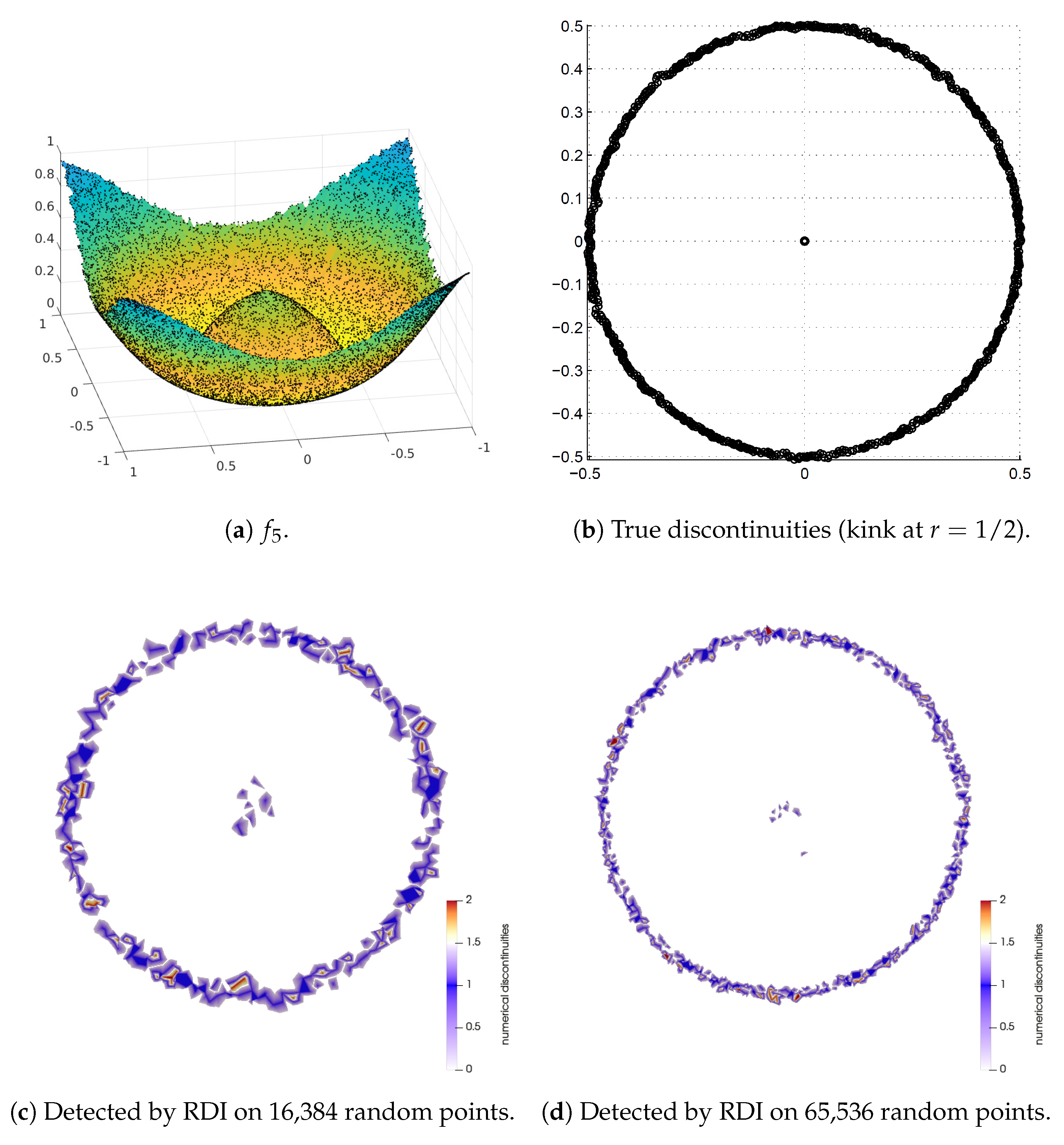
5.1. Experimentation on Unit Spheres with Nonuniform Neshes

To evaluate our discontinuity indicators, we employed two piecewise smooth functions, “interacting waves” and “crossing waves,” which were previously used in [13]. The definitions of these functions are as follows:

$$f_1\left(\theta ,\phi \right)=\left\{\begin{array}{cc}1,\hfill & \mathrm{if}0\le \theta <5\pi /18,\hfill \\ 1.7-2.52\theta /\pi ,\hfill & \mathrm{if}5\pi /18\le \theta <\pi /2,\hfill \\ 0.44,\hfill & \mathrm{if}\pi /2\le \theta <13\pi /18,\hfill \\ 0.24,\hfill & \mathrm{if}13\pi /18\le \theta <9\pi /10,\hfill \\ 0.12,\hfill & \mathrm{if}9\pi /10\le \theta \le \pi ,\hfill \end{array}\right.$$

and

$$f_2\left(\theta ,\phi \right)=-1000+2000\mathrm{sign}(cos\left(\phi \right))\left\{\begin{array}{cc}1/2,\hfill & \mathrm{if}0\le \theta <\pi /4,\hfill \\ -4\left(\theta /\pi -1/2\right),\hfill & \mathrm{if}\pi /4\le \theta <\pi /2,\hfill \\ 4\left(\theta /\pi -1/2\right),\hfill & \mathrm{if}\pi /2\le \theta <3\pi /4,\hfill \\ 1,\hfill & \mathrm{if}3\pi /4\le \theta <7\pi /8,\hfill \\ -64{\theta }^2/{\pi }^2+112\theta /\pi -48,\hfill & \mathrm{if}7\pi /8\le \theta \le \pi .\hfill \end{array}\right.$$

Note that $f_1$ has $C^0$ and $C^1$ discontinuities, whereas $f_2$ has $C^0$, $C^1$, and $C^2$ discontinuities. We chose these functions since the discontinuities have complex interacting patterns, allowing a more thorough evaluation of the robustness of the indicators. Figure 1 displays the color maps of the two functions on two regionally refined meshes. Specifically, $f_1$ is shown on the dual of a spherical centroidal Voronoi tessellations (SCVT) mesh [46], and $f_2$ is shown on a cubed-sphere mesh. The meshes in Figure 1 are relatively coarse. For ease of visualization, we intersect the sphere with planes and will depict the values on the intersection curves henceforth.

Figure 1. Function values on coarse regionally refined meshes and the intersection planes. (a) $f_1$ on the dual of a coarse regionally refined SCVT ($N_v=$ 31,936, $N_c=$ 15,970) with the intersection plane $x+y=0$. (b) $f_2$ on a coarse regionally refined cubed-sphere ($N_v=$ 15,860, $N_c=$ 15,858) with the intersection plane $y-2x=0$.

Figure 2 depicts the function values and ${\beta }_v$ values along the intersection curves on finer meshes, which have edge lengths of approximately one-fourth of those seen in Figure 1. We use $N_v$ and $N_c$ to denote the number of vertices and cells, respectively, in the meshes. It is evident that the ${\beta }_v$ values can effectively distinguish the discontinuities from the smooth regions. Figure 3 shows the nodes where ${\eta }_v\ge 1$ (i.e., ${\beta }_v>{\kappa }_1=0.5$, assuming ${\kappa }_0$ is larger). These nodes correspond to the regions with $C^0$ and $C^1$ discontinuities. For these tests, we used ${\kappa }_1=0.5$, ${\kappa }_0=1.5$, $C_{\ell }=0.4$, $C_g=0.05$. Reducing ${\kappa }_1$ to a smaller value may allow for the identification of some $C^2$ discontinuities on coarse meshes but would also increase the risk of false positives.

Figure 2. Functions $f_1$ and $f_2$ along with their corresponding ${\beta }_v$ values along the cross section of finer regionally refined meshes (SCVT: $N_v=$ 135,768, $N_c=$ 67,886; cubed-sphere: $N_v=$ 247,330, $N_c=$ 247,328) with intersection planes.

Figure 3. Detected discontinuity cells (cells incident to nodes with ${\eta }_v\ge 1$, shown in red) on regionally refined meshes. (a) Detected discontinuity cells of $f_1$ on level-3 regionally refined SCVT ($N_v=$ 135,768, $N_c=$ 67,886). (b) Detected discontinuity cells of $f_2$ on level-3 regionally refined cubed-sphere mesh ($N_v=$ 247,330, $N_c=$ 247,328).

5.2. Comparison with Polynomial Annihilation Edge Detection

We compare RDI with Polynomial Annihilation Edge Detector (PAED) [22,23]. Like RDI, PAED is designed to detect discontinuities in functions, primarily $C^0$ discontinuities in its original formulation [22] and extended to $C^1$ discontinuities by applying it to estimated derivatives [23]. PAED is based on polynomial annihilation and often uses limiters like the minmod limiter [47,48] to reduce oscillations when approximating jump functions or derivatives. Since PAED is typically formulated for 2D planar data, we conduct the comparison on planar domains.

First, we use two test functions, $f_3$ and $f_4$, from [22], both of which contain only $C^0$ discontinuities. Specifically, the function $f_3$ is given by

$$f_3(x,y)=\left\{\begin{array}{cc}xy+cos\left(2\pi x^2\right)-sin\left(2\pi x^2\right),\hfill & \mathrm{if}{x}^2+y^2\le {\displaystyle \frac{1}{4}},\hfill \\ 10x-5+xy+cos\left(2\pi x^2\right)-sin\left(2\pi x^2\right),\hfill & \mathrm{if}{x}^2+y^2>{\displaystyle \frac{1}{4}},\hfill \end{array}\right.$$

for $-1\le x,y\le 1$, and $f_4$ is the gray level of the Shepp–Logan phantom [49].

For comparison with [22], we generated 16,384 random points on $[-1,1]\times [-1,1]$. As RDI uses a mesh data structure for computing neighborhoods, we computed the Delaunay triangulation of these points when applying RDI. To visualize the detected discontinuities, we computed an approximation of the local jump function

$$\delta f\left(\mathit{x}\right)=\left\{\begin{array}{cc}\underset{\mathit{y}\in R\left(\mathit{x}\right)}{max}f\left(\mathit{y}\right)-\underset{\mathit{y}\in R\left(\mathit{x}\right)}{min}f\left(\mathit{y}\right),\hfill & \mathrm{if}\mathrm{node}\mathit{x}\mathrm{is}\mathrm{marked}\mathrm{by}\mathrm{RDI}(\mathrm{i}.\mathrm{e}.,{\eta }_x\ge 1),\hfill \\ 0,\hfill & \mathrm{otherwise},\hfill \end{array}\right.$$

where $R\left(\mathit{x}\right)$ is the one-ring neighborhood of nodes connected to $\mathit{x}$ (including $\mathit{x}$) on the sampled mesh.

Figure 4 displays the results, which are visually similar to those for the PAED method shown in Figures 4.2 and 4.3 of [22]. Subplots (a) and (c) show the original functions $f_3$ and $f_4$, where both height (z-axis) and color represent the function’s value. Subplots (b) and (d) visualize the output of our RDI method by plotting the local jump function $\delta f$. In these plots, the non-zero regions trace the detected $C^0$ discontinuities. Both the height and the color of the resulting surfaces correspond to the magnitude of the local jump, accurately aligning with the true discontinuities in the original functions. For instance, the constant-height (and single-color) circular wall in (b) reflects the constant jump in $f_3$, while the varying heights (and colors) in (d) correctly capture the different jump magnitudes in the Shepp–Logan phantom.

Figure 4. Original functions (a) $f_3$ and (c) $f_4$, and their approximated local jump functions (b,d) based on RDI detection (on Delaunay triangulation of 16,384 random points), respectively.

The detected discontinuities from PAED may appear thinner in some cases than those of RDI, partly because RDI uses larger stencils (two rings for the OSUS operator), which can slightly widen the detected region around a discontinuity. RDI parameters for this test were ${\kappa }_1=0.3$ and ${\kappa }_0=1.0$.

A key feature of RDI is its ability to detect both $C^0$ and $C^1$ discontinuities in a single pass without prior derivative estimation. In [23], PAED was extended to detect $C_1$ discontinuities by first estimating the derivatives and then applying PAED to these derivative fields. To compare our method with [23], we use the test function $f_5$ from their work,

$$f_5(x,y)=\left\{\begin{array}{cc}-\left(\sqrt{x^2+y^2}-{\displaystyle \frac{1}{2}}\right)+{\displaystyle \frac{1}{12}}sin\left(2\pi \sqrt{x^2+y^2}\right),\hfill & \mathrm{if}\sqrt{x^2+y^2}<{\displaystyle \frac{1}{2}},\hfill \\ \left(\sqrt{x^2+y^2}-{\displaystyle \frac{1}{2}}\right)+{\displaystyle \frac{1}{12}}sin\left(2\pi \sqrt{x^2+y^2}\right),\hfill & \mathrm{if}\sqrt{x^2+y^2}\ge {\displaystyle \frac{1}{2}},\hfill \end{array}\right.$$

which has a $C_1$ discontinuity (a kink) along the circle $\sqrt{x^2+y^2}=1/2$. We generated meshes over $[-1,1]\times [-1,1]$ of similar point counts as those in [23]. As shown in Figure 5, our RDI method detected the $C^1$ discontinuity along the circle with high fidelity and very few false positives. In contrast, the results reported for the two-pass PAED approach in [23] (see their Figure 8) exhibit numerous false positives scattered across the domain, particularly on the random grids. This comparison suggests that RDI’s direct, single-pass approach is more robust for detecting $C^1$ discontinuities, likely because it avoids a separate, potentially noise-sensitive derivative estimation step.

Figure 5. Detection of the $C_1$ discontinuity in $f_5$ using the RDI method on the Delaunay triangulation of two different random point sets. The method cleanly identifies the circular discontinuity with very few false positives.

5.3. Generalization to Surfaces with Sharp Features

Our previous examples employed simple, smooth geometries, such as spheres and planes. We now consider surfaces with sharp features, which present additional complications. As discussed in Section 4.3 and detailed in [20], we virtually split the surface mesh into smooth patches along the feature curves and then employ one-sided stencils (by restricting stencils to the patch) along these sharp features. The virtual splitting helps to prevent many false positives and negatives, as demonstrated in Appendix B. To maintain stability, we increase the stencil sizes (e.g., to 3-rings) for WLS near the patch boundaries when computing the OSUS operator, as discussed in Section 4.3.

We carried out several experiments and displayed the results for functions $f_6$ and $f_7$ (defined below) on complex geometries. The functions are as follows:

$$f_6(x,y,z)=tanh\left(x\right)\mathrm{sign}\left(y\right)+tanh\left(y\right)\mathrm{sign}\left(z\right)+tanh\left(z\right)\mathrm{sign}\left(x\right),$$

and

$$f_7(x,y,z)=(\underset{\mathrm{domain}}{max}\left\{x\right\}-\underset{\mathrm{domain}}{min}\left\{x\right\})g\left({\displaystyle \frac{x-{min}_{\mathrm{domain}}\left\{x\right\}}{{max}_{\mathrm{domain}}\left\{x\right\}-{min}_{\mathrm{domain}}\left\{x\right\}}}\right),$$

respectively, where ${max}_{\mathrm{domain}}\left\{x\right\}$ and ${min}_{\mathrm{domain}}\left\{x\right\}$ are taken over the coordinate range of the specific geometry, and

$$g\left(s\right)=\left\{\begin{array}{cc}s,\hfill & \mathrm{if}0\le s<{\displaystyle \frac{1}{4}},\hfill \\ {\displaystyle \frac{1}{2}}-s,\hfill & \mathrm{if}{\displaystyle \frac{1}{4}}\le s<{\displaystyle \frac{1}{2}},\hfill \\ {\displaystyle \frac{3}{4}},\hfill & \mathrm{if}{\displaystyle \frac{1}{2}}\le s<{\displaystyle \frac{3}{4}},\hfill \\ 16{(s-{\displaystyle \frac{3}{4}})}^3+{\displaystyle \frac{3}{4}},\hfill & \mathrm{if}{\displaystyle \frac{3}{4}}\le s\le 1.\hfill \end{array}\right.$$

Function $f_6$ has $C^0$ discontinuities along the planes $y=0,z=0,x=0$. Function $f_7$ has $C^0$ and $C^1$ discontinuities based on the x-coordinate.

Figure 6 and Figure 7 display the detected discontinuities on a cylinder and a reamer, respectively. It can be observed that RDI accurately detected the $C^0$ discontinuities. Some $C^1$ discontinuities might be missed if the quadratic WLS had minimal overshoots and undershoots for the given mesh resolution in the corresponding regions, leading to small ${\alpha }_{\sigma }$ and subsequently small ${\beta }_v$. Decreasing the threshold ${\kappa }_1$ would make RDI more sensitive to weaker $C^1$ discontinuities, although it may also introduce some false positives in regions of high smooth variation.

Figure 6. Function values and numerical discontinuities (red regions indicate ${\eta }_v\ge 1$) detected by RDI with virtual splitting on the surface triangulations of a cylinder ($N_v=$ 20,177, $N_c=$ 39,788).

Figure 7. Function values and numerical discontinuities (red regions indicate ${\eta }_v\ge 1$) detected by RDI with virtual splitting on the surface triangulation of a reamer ($N_v=$ 19,515, $N_c=$ 33,246).

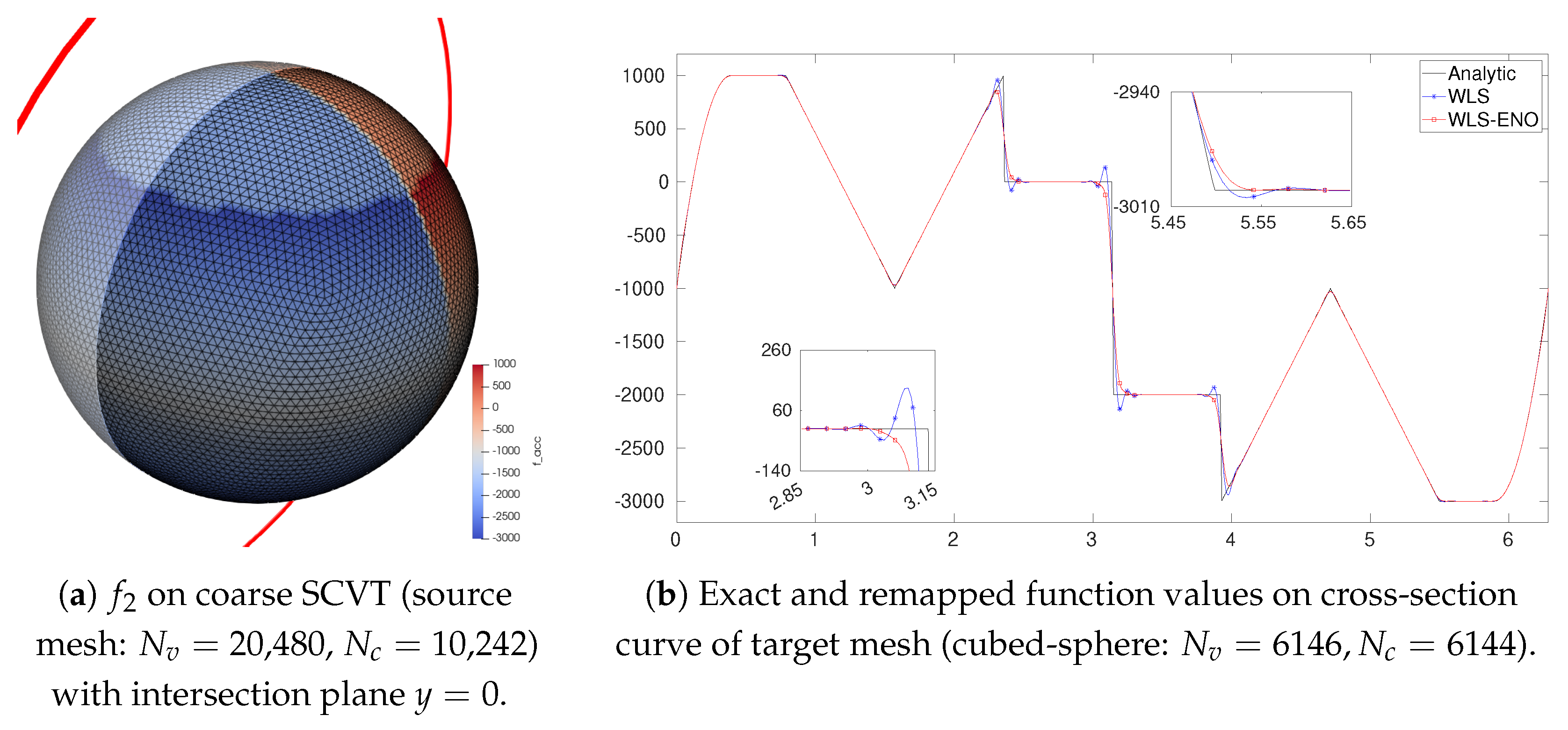
5.4. Application to Remap

The robust detection of discontinuities has a variety of applications. In this section, we demonstrate the use of RDI in remapping data between different meshes, also known as data remap or conservative interpolation. In this context, upon identifying $C^0$ and $C^1$ discontinuities using RDI, one can employ specialized numerical techniques, such as WLS-ENO remap [13,20] or CAAS [50], to resolve or limit across these discontinuities, thereby mitigating the Gibbs phenomena [4]. Figure 8 compares the remapping of $f_2$ (from Section 5.1) from a source SCVT mesh to a target cubed-sphere mesh using standard WLS interpolation versus a WLS-ENO scheme that utilizes RDI markers. The standard WLS, which does not distinguish smooth and discontinuous regions, suffers from oscillations near discontinuities. In contrast, WLS-ENO, guided by RDI to adjust its stencils and weights near detected discontinuities, effectively eliminated overshoots and undershoots while preserving accuracy in smooth regions.

Figure 8. Comparison between standard WLS interpolation and WLS-ENO (using RDI) for remapping $f_2$. (a) $f_2$ on the source mesh. (b) Function profiles along a cross-section of the target mesh: exact solution (black), standard WLS remapped (blue, oscillatory), and WLS-ENO with RDI remapped (red, non-oscillatory).

6. Conclusions and Discussion

In this paper, we have introduced the Robust Discontinuity Indicators (RDI) method, a novel approach for the robust and efficient detection of discontinuities in approximating piecewise continuous functions over meshes. The RDI method distinguishes itself by accurately identifying both $C^0$ and $C^1$ discontinuities using node-based values, even in nonuniform meshes and complex surface geometries. Our approach leverages a combination of cell-based overshoot–undershoot indicators (${\alpha }_{\sigma }$) and node-based oscillation indicators (${\beta }_v$), processed through a dual-thresholding strategy, ensuring robustness while minimizing false positives. The theoretical foundation provided by our rigorous analysis of WLS and linear interpolation behavior near discontinuities, coupled with extensive numerical experiments, demonstrates that RDI achieves high accuracy in discontinuity detection and maintains computational efficiency across a wide range of scenarios. The ability to precompute the main OSUS operator makes RDI particularly efficient for applications involving multiple functions on a fixed mesh.

Despite the promising results obtained, there are avenues for further enhancement. One potential improvement could involve incorporating a thinning process post-detection to refine the boundaries of the detected discontinuities. Extending the RDI method to three-dimensional volumetric meshes could broaden its applicability. Further investigation into the adaptive determination of the thresholds (${\kappa }_0,{\kappa }_1,C_{\ell },C_g$) could also improve robustness across a wider range of functions and meshes without manual tuning.

Beyond these direct improvements, our work opens up several avenues for future research. One direction is to reconstruct topologically correct discontinuity curves from the discrete points identified by RDI, a challenge relevant to applications in geometric modeling [51]. Another avenue is adapting RDI’s principles for 1D event detection in ODEs and DAEs. Such a tool would complement existing methods [8] and is critical because improper regularization can alter the qualitative dynamics of piecewise-smooth (PWS) systems, such as their limit cycles [7,52].

References

- Hesthaven, J.S.; Warburton, T. Nodal Discontinuous Galerkin Methods; Springer: Berlin/Heidelberg, Germany, 2008. [Google Scholar]
- Botsch, M.; Kobbelt, L.; Pauly, M.; Alliez, P.; Lévy, B. Polygon Mesh Processing; CRC Press: Boca Raton, FL, USA, 2010. [Google Scholar]
- LeVeque, R.J. Finite Volume Methods for Hyperbolic Problems; Cambridge University Press: Cambridge, UK, 2002. [Google Scholar]
- Gottlieb, D.; Shu, C.W. On the Gibbs phenomenon and its resolution. SIAM Rev. 1997, 39, 644–668. [Google Scholar] [CrossRef]
- Shu, C.W. High order ENO and WENO schemes for computational fluid dynamics. In High-Order Methods for Computational Physics; Springer: Berlin/Heidelberg, Germany, 1999; pp. 439–582. [Google Scholar]
- Liu, X.D.; Osher, S.; Chan, T. Weighted essentially non-oscillatory schemes. J. Comput. Phys. 1994, 115, 200–212. [Google Scholar] [CrossRef]
- Dieci, L.; Guglielmi, N. Regularizing Piecewise Smooth Differential Systems: Co-Dimension Discontinuity Surface. J. Dyn. Differ. Equ. 2013, 25, 71–94. [Google Scholar] [CrossRef]
- Lopez, L.; Maset, S. Numerical event location techniques in discontinuous differential algebraic equations. Appl. Numer. Math. 2022, 178, 98–122. [Google Scholar] [CrossRef]
- Harten, A. ENO schemes with subcell resolution. J. Comput. Phys. 1989, 83, 148–184. [Google Scholar] [CrossRef]
- Jiang, G.S.; Peng, D. Weighted ENO Schemes for Hamilton–Jacobi Equations. SIAM J. Sci. Comput. 2000, 21, 2126–2143. [Google Scholar] [CrossRef]
- Amat, S.; Ruiz, J. New WENO Smoothness Indicators Computationally Efficient in the Presence of Corner Discontinuities. J. Sci. Comput. 2017, 71, 1265–1302. [Google Scholar] [CrossRef]
- Liu, H.; Jiao, X. WLS-ENO: Weighted-least-squares based essentially non-oscillatory schemes for finite volume methods on unstructured meshes. J. Comput. Phys. 2016, 314, 749–773. [Google Scholar] [CrossRef]
- Li, Y.; Chen, Q.; Wang, X.; Jiao, X. WLS-ENO remap: Superconvergent and non-oscillatory weighted least squares data transfer on surfaces. J. Comput. Phys. 2020, 417, 109578. [Google Scholar] [CrossRef]
- Tadmor, E. Filters, mollifiers and the computation of the Gibbs phenomenon. Acta Numer. 2007, 16, 305–378. [Google Scholar] [CrossRef]
- Cates, D.; Gelb, A. Detecting derivative discontinuity locations in piecewise continuous functions from Fourier spectral data. Numer. Algo. 2007, 46, 59–84. [Google Scholar] [CrossRef]
- Hewitt, E.; Hewitt, R.E. The Gibbs-Wilbraham phenomenon: An episode in Fourier analysis. Arch. Hist. Exact Sci. 1979, 21, 129–160. [Google Scholar] [CrossRef]
- Bozzini, M.; Rossini, M. The detection and recovery of discontinuity curves from scattered data. J. Comput. Appl. Math. 2013, 240, 148–162. [Google Scholar] [CrossRef]
- de Silanes, M.C.L.; Parra, M.C.; Torrens, J.J. Vertical and oblique fault detection in explicit surfaces. J. Comput. Appl. Math. 2002, 140, 559–585. [Google Scholar] [CrossRef]
- Moura, R.C.; Cassinelli, A.; da Silva, A.F.; Burman, E.; Sherwin, S.J. Gradient jump penalty stabilisation of spectral/hp element discretisation for under-resolved turbulence simulations. Comput. Methods Appl. Mech. Eng. 2022, 388, 114200. [Google Scholar] [CrossRef]
- Li, Y.; Zhao, X.; Ray, N.; Jiao, X. Compact feature-aware Hermite-style high-order surface reconstruction. Engrg. Comput. 2021, 37, 187–210. [Google Scholar] [CrossRef]
- Shrivakshan, G.T. A comparison of various edge detection techniques used in image processing. Int. J. Comput. Sci. Issues 2012, 9, 269. [Google Scholar]
- Archibald, R.; Gelb, A.; Yoon, J. Polynomial fitting for edge detection in irregularly sampled signals and images. SIAM J. Numer. Ana. 2005, 43, 259–279. [Google Scholar] [CrossRef]
- Saxena, R.; Gelb, A.; Mittelmann, H. A high order method for determining the edges in the gradient of a function. Comm. Comput. Phys. 2009, 5, 694–711. [Google Scholar]
- Archibald, R.; Gelb, A.; Yoon, J. Determining the locations and discontinuities in the derivatives of functions. Appl. Numer. Math. 2008, 58, 577–592. [Google Scholar] [CrossRef]
- Glaubitz, J.; Gelb, A. High Order Edge Sensors with ℓ1 Regularization for Enhanced Discontinuous Galerkin Methods. SIAM J. Sci. Comput. 2019, 41, A1304–A1330. [Google Scholar] [CrossRef]
- Marr, D.; Hildreth, E. Theory of edge detection. Proc. Roy. Soc. Lond. 1980, 207, 187–217. [Google Scholar]
- Marr, D. Early processing of visual information. Philos. Trans. R. Soc. Lond. B Biol. Sci. 1976, 275, 483–519. [Google Scholar]
- Marr, D.; Ullman, S.; Poggio, T. Bandpass channels, zero-crossings, and early visual information processing. J. Opt. Soc. Am. 1979, 69, 914–916. [Google Scholar] [CrossRef]
- Mallat, S.; Hwang, W.L. Singularity detection and processing with wavelets. IEEE Trans. Inf. Theory 1992, 38, 617–643. [Google Scholar] [CrossRef]
- Rossini, M. Interpolating functions with gradient discontinuities via Variably Scaled Kernels. Dolomites Res. Notes Approx. 2018, 11, 3–14. [Google Scholar]
- De Marchi, S.; Marchetti, F.; Perracchione, E.; Poggiali, D. Polynomial interpolation via mapped bases without resampling. J. Comput. Appl. Math. 2020, 364, 112347. [Google Scholar] [CrossRef]
- Gelb, A.; Tadmor, E. Detection of edges in spectral data. Appl. Comput. Harmon. Anal. 1999, 7, 101–135. [Google Scholar] [CrossRef]
- Gelb, A.; Tadmor, E. Detection of edges in spectral data II. Nonlinear enhancement. SIAM J. Numer. Anal. 2000, 38, 1389–1408. [Google Scholar] [CrossRef]
- Jiao, X.; Zha, H. Consistent computation of first- and second-order differential quantities for surface meshes. In Proceedings of the ACM Solid and Physical Modeling Symposium, Stony Brook, NY, USA, 2–4 June 2008; pp. 159–170. [Google Scholar]
- Buhmann, M.D. Radial Basis Functions: Theory and Implementations; Cambridge University Press: Cambridge, UK, 2003; Volume 12. [Google Scholar]
- Hu, C.; Shu, C.W. Weighted essentially non-oscillatory schemes on triangular meshes. J. Comput. Phys. 1999, 150, 97–127. [Google Scholar] [CrossRef]
- Shi, J.; Hu, C.; Shu, C.W. A technique of treating negative weights in WENO schemes. J. Comput. Phys. 2002, 175, 108–127. [Google Scholar] [CrossRef]
- Xu, Z.; Liu, Y.; Du, H.; Lin, G.; Shu, C.W. Point-wise hierarchical reconstruction for discontinuous Galerkin and finite volume methods for solving conservation laws. J. Comput. Phys. 2011, 230, 6843–6865. [Google Scholar] [CrossRef]
- Zhang, Y.T.; Shu, C.W. Third order WENO scheme on three dimensional tetrahedral meshes. Comm. Comput. Phys. 2009, 5, 836–848. [Google Scholar]
- Liu, Y.; Zhang, Y.T. A robust reconstruction for unstructured WENO schemes. J. Sci. Comput. 2013, 54, 603–621. [Google Scholar] [CrossRef]
- Jiao, X.; Wang, D. Reconstructing high-order surfaces for meshing. Engrg. Comput. 2012, 28, 361–373. [Google Scholar] [CrossRef]
- Ray, N.; Wang, D.; Jiao, X.; Glimm, J. High-Order Numerical Integration over Discrete Surfaces. SIAM J. Numer. Anal. 2012, 50, 3061–3083. [Google Scholar] [CrossRef]
- Buhmann, M. A new class of radial basis functions with compact support. Math. Comput. 2001, 70, 307–318. [Google Scholar] [CrossRef]
- Dyedov, V.; Ray, N.; Einstein, D.; Jiao, X.; Tautges, T. AHF: Array-Based Half-Facet Data Structure for Mixed-Dimensional and Non-manifold Meshes. In Proceedings of the 22nd International Meshing Roundtable, Orlando, FL, USA, 13–16 October 2013; Sarrate, J., Staten, M., Eds.; Springer International Publishing: Berlin/Heidelberg, Germany, 2014; pp. 445–464. [Google Scholar]
- Li, Y.; Jiao, X. Mesh used for Robust Discontinuity Indicators workflows. arXiv 2024, arXiv:2308.02235. [Google Scholar]
- Ju, L.; Ringler, T.; Gunzburger, M. Voronoi tessellations and their application to climate and global modeling. In Numerical Techniques for Global Atmospheric Models; Springer: Berlin/Heidelberg, Germany, 2011; pp. 313–342. [Google Scholar]
- Roe, P.L.; Baines, M.J. Algorithms for advection and shock problems. In Proceedings of the 4th Conference on Numerical Methods in Fluid Mechanics, Paris, France, 7–9 October 1981; pp. 281–290, Conference held in 1981, proceedings published in 1982. [Google Scholar]
- Gelb, A.; Tadmor, E. Adaptive edge detectors for piecewise smooth data based on the minmod limiter. J. Sci. Comput. 2006, 28, 279–306. [Google Scholar] [CrossRef]
- Shepp, L.A.; Logan, B.F. The Fourier reconstruction of a head section. IEEE Trans. Nucl. Sci. 1974, 21, 21–43. [Google Scholar] [CrossRef]
- Bradley, A.M.; Bosler, P.A.; Guba, O.; Taylor, M.A.; Barnett, G.A. Communication-efficient property preservation in tracer transport. SIAM J. Sci. Comput. 2019, 41, C161–C193. [Google Scholar] [CrossRef]
- Difonzo, F.V. Isochronous attainable manifolds for piecewise smooth dynamical systems. Qual. Theory Dyn. Syst. 2022, 21, 6. [Google Scholar] [CrossRef]
- Pi, D. Limit cycles for regularized piecewise smooth systems with a switching manifold of codimension two. Discret. Contin. Dyn. Syst. Ser. B 2019, 24, 881–905. [Google Scholar] [CrossRef]
Disclaimer/Publisher’s Note: The statements, opinions and data contained in all publications are solely those of the individual author(s) and contributor(s) and not of MDPI and/or the editor(s). MDPI and/or the editor(s) disclaim responsibility for any injury to people or property resulting from any ideas, methods, instructions or products referred to in the content. |
© 2025 by the authors. Licensee MDPI, Basel, Switzerland. This article is an open access article distributed under the terms and conditions of the Creative Commons Attribution (CC BY) license (https://creativecommons.org/licenses/by/4.0/).