CIRGNN: Leveraging Cross-Chart Relationships with a Graph Neural Network for Stock Price Prediction

Abstract

Recent years have seen a rise in combining deep learning and technical analysis for stock price prediction. However, technical indicators are often prioritized over technical charts due to quantification challenges. While some studies use closing price charts for predicting stock trends, they overlook charts from other indicators and their relationships, resulting in underutilized information for predicting stock. Therefore, we design a novel framework to address the underutilized information limitations within technical charts generated by different indicators. Specifically, different sequences of stock indicators are used to generate various technical charts, and an adaptive relationship graph learning layer is employed to learn the relationships among technical charts generated by different indicators. Finally, by applying a GNN model combined with the relationship graphs of diverse technical charts, temporal patterns of stock indicator sequences are captured, fully utilizing the information between various technical charts to achieve accurate stock price predictions. Additionally, we further tested our framework with real-world stock data, showing superior performance over advanced baselines in predicting stock prices, achieving the highest net value in trading simulations. Our research results not only complement the existing applications of non-singular technical charts in deep learning but also offer backing for investment applications in financial market decision-making.

1. Introduction

Technical analysis (TA) is a widely used methodology for evaluating financial assets based on historical price and volume data, and it plays a central role in financial trading. Given that TA revolves around the belief that all relevant information for investment decision-making is encapsulated within technical indicators and technical charts, traders rely on these tools to thoroughly analyze market trends and develop effective trading strategies [1]. In recent years, an increasing number of technical analysts have adopted advanced deep learning methods for stock price prediction [2].

Technical charts can be as informative as technical indicators for stock price prediction in traditional, non-deep-learning settings [3]. However, in quantitative trading and machine learning applications, technical indicators are generally preferred over technical charts due to their inherent numerical properties and ease of standardization [4]. Indicators can be directly integrated into learning models as structured features, offering consistency across datasets. In contrast, technical charts contain complex visual patterns that are challenging to quantify and algorithmically process, largely because of scale variations, noise, and the subjectivity involved in human pattern recognition [5,6]. As a result, existing algorithmic approaches often underutilize the potentially valuable information embedded in chart structures. Despite evidence that some specific chart patterns can enhance profitability, their effectiveness is often limited to certain market contexts or periods [7]. To address the challenges associated with applying technical charts in deep learning, recent researchers have transformed closing price series into graph structures to extract general technical chart information [8]. These works primarily focus on the structural information in closing prices, but often neglect comparable information from other indicators and charts. Moreover, they overlook the relationships between technical charts derived from different indicators, which may result in missed opportunities to leverage the rich interconnections embedded in diverse financial signals. On the one hand, technical charts of other price series (except close price) or technical indicators also contain important information. For instance, the development of some technical charts are supported by an upward trend in volume [9]. An increase in volume indicates the emergence of some charts. On the other hand, technical charts derived from multiple stock indicators contain valuable market information beyond single indicator analysis alone. these charts are not isolated but exhibit meaningful interactions and directional relationships. Explicitly capturing these cross-chart relationships is therefore crucial for understanding the dynamic information flows underlying stock market movements and improving the accuracy of stock price predictions. Although some researchers have explored the relationships between technical indicators and stock prices [4], there are still deficiencies in the research field regarding the exploration of connections among different technical charts generated from various indicators of the stock.

Recent research has emphasized the importance of exploring relationships between technical charts across different indicators to enhance trading strategies for technical analysts. For example, analysts can validate buy or sell signals generated by technical indicators against chart patterns or trend lines from various charts, improving the reliability of trading signals [10]. Moreover, researchers have explored correlations between different technical charts derived from stock prices to devise dynamic trading strategies [11]. Despite these advances, many existing approaches still focus on individual charts or isolated indicators, overlooking the structural information that emerges when multiple technical charts are considered jointly. Even when some cross-chart relationships are identified, integrating such dependencies into predictive models remains a significant challenge. Identifying such connections is crucial for improving stock price prediction, yet developing robust methods to leverage these relationships for enhanced forecasting performance is still an open problem. In response to this challenge, graph neural networks (GNNs) have emerged as promising tools for modeling complex relationships between entities [12], offering new perspectives on capturing and utilizing dependencies between technical indicators and chart patterns.

To address the issues mentioned above, we design a new framework named Chart Indicator Relationship Graph Neural Network (CIRGNN), which aims to fully leverage the chart information within various indicators while exploring the relationships among different indicator charts. Initially, we utilize the visibility graph (VG) algorithm [13] to transform various indicator sequences into graph structures, thereby extracting common chart information from different indicators. Subsequently, we devise an adaptive relationship graph learning layer to obtain the connections between the transformed graphs of different indicators, delineating the relationships among different indicator charts. Finally, a GNN model comprising temporal convolution modules and graph convolution modules is employed for capturing temporal patterns in the stock series and analyze information among indicators, stock series, and charts for accurate stock price prediction. Distinct from prior works such as Chart-GCN, which represent only a single technical indicator (typically the closing price) as a graph, our framework systematically constructs graphs for multiple technical charts derived from diverse indicators and, crucially, learns the directed and dynamic relationships among them. This cross-chart relational modeling enables our approach to capture complex, context-dependent dependencies that are essential in practical financial forecasting, representing a substantial methodological advancement in the field. On our collected dataset, our proposed framework attained the highest prediction performance, with a predicted MAPE of 0.0473. Based on the stock price prediction results obtained from our method, we devise trading strategies for the selected stocks, resulting in the highest net value achievement in 2022, which is 1.095. Furthermore, we provide visualization results of the graphs learned in the model and offer reasonable interpretations of the graphs.

In summary, the primary contributions of this paper include the following:

• A new framework is proposed to fully employ both technical charts and technical indicators for predicting stock price.
• Our methods involve exploring the relationship between technical charts and indicators, overcoming the limitation of relying solely on specific charts in deep learning.
• Our framework outperforms the baseline methods in prediction accuracy. We also attain the utmost excess return in the actual stock market.

The organization of the remaining sections of this paper is as follows: Section 2 introduces the related work. In Section 3, the details of our proposed methods are reported. Section 4 illustrates the experimental settings and showcases the results. Section 5 elaborates the results. Section 6 presents the conclusions.

2. Related Work

2.1. Technical Charts

In financial market analysis, technical chart analysis emerges as a crucial methodology, extensively utilized for predicting stock prices. It is characterized by the connection of price points using lines and requires the employment of pattern recognition methodologies by technical analysts to identify appropriate charts guiding trading strategy. In stock movement prediction, numerous research endeavors rely on pattern-matching technology to examine patterns seen in past stock price charts [14]. They aim to determine whether or not current stock prices show comparable patterns, like ‘rounding bottoms’, ‘bull flags’, or ‘head-and-shoulders’ [15]. Recent studies have meticulously examined particular charts manifested in historical stock price series and quantified them in order to determine whether or not current stock prices demonstrate similarities to established trends, applying these quantified charts in deep learning. For example, to discern current stock price series charts, scholars have dedicated themselves to exploring similarity methods like the Pearson correlation coefficient and dynamic time warping, which evaluate the likeness between charts identified within previous data or curated by specialists and the present stock price sequences [16]. Moreover, by converting market price series into graphs and extracting structural information, some researchers have enhanced the accuracy of stock price predictions by addressing long-term dependencies and chaotic properties [8]. Additionally, others have extracted key point sequences from stock price series and employed graph convolutional networks (GCNs) and other graph kernels to fully exploit chart information for stock movement forecasting [7]. However, while the methods proposed by these studies address some of the issues with the use of technical charts in deep learning, for predicting stock price, they only utilize technical charts generated from closing prices, overlooking the application of technical charts based on other indicators. Thus, they fail to fully utilize the valuable information contained within the various technical charts derived from technical indicators for accurate stock price prediction.

To address the issue, we utilize the VG algorithm [13], a methodology aimed at transforming time-series data into intricate network representations to effectively convert different stock indicators into technical charts represented by graphs, thus harnessing the structural information contained in the charts. The relationships between technical charts generated from different indicators also contain important information about stock price changes. Therefore, we must also fully consider the relationships between charts in our research.

2.2. Graph Learning for Stock Prediction

Lately, the progress in deep learning has brought GNNs to the forefront as a powerful method for handling dependency relationships between different entities and temporal dynamics. Graph neural networks operate under the assumption that node status is influenced by the status of its neighboring nodes. In order to grasp such spatial dependencies, researchers have devised a range of graph neural networks utilizing techniques such as message passing [17], information propagation [18], and graph convolution [19]. These networks function similarly, fundamentally capturing advanced node representations by disseminating the states of neighboring nodes to the nodes themselves. Existing studies often utilize knowledge graphs to store and depict these relationships. For example, a study organizes industry relationships among entities into knowledge graphs and predicts stock movements by utilizing graph networks [20]. Additionally, researchers also construct multi-modality graph neural networks using historical stock price sequences, media news about companies, and correlative events [21]. However, the actual graph will frequently change over time along with fluctuations in the financial markets. The graphs constructed by the aforementioned methods are limited by the unaltered, predefined relationships chosen subjectively by researchers. Furthermore, the graph construction methods mentioned above do not incorporate technical charts and indicators. Therefore, existing methods do not fully utilize all the information in the stock data. Furthermore, some researchers have attempted to design a class of universal GNN frameworks for multivariate time-series data [22]. This method automatically extracts relationships among variables using the graph learning module, facilitating the integration of external knowledge, like variable attributes. Inspired by this, we can design a module in our framework to automatically learn the relationships between technical charts generated from different stock indicators. Some studies also suggest that GNNs can simultaneously capture the local and global information of the entire graph, thereby better understanding the relationships between nodes [23]. GNNs, by means of employing a message-passing mechanism, facilitate the dissemination of information across graph structures. Each node updates its features by incorporating information from its neighboring nodes. Additionally, it captures the local information of nodes through local convolutions and gradually integrates node features through multiple convolution layers, propagating them across the entire graph to acquire global information [24]. Additionally, GNNs exhibit robust scalability and adaptability, enabling them to dynamically modify both the architecture and parameters of the model to suit diverse prediction tasks and data characteristics. Thus, they are applicable to prediction tasks. Inspired by this, incorporating a GNN into our framework can fully exploit information from technical charts and indicators in predicting stock price using input stock sequences.

3. Method

In this research, we design a new method, named the Chart Indicator Relation Graph Neural Network (CIRGNN), to predict stock prices. Our approach utilizes the VG algorithm and adaptive relationship graph learning layer to thoroughly explore chart and indicator information. This new framework aims to address the limitations inherent in existing methods that inadequately utilize the information within technical charts generated by stock indicators, as well as their interrelationships.

The Figure 1 shows how our framework predicts the stock prices. Specifically, we first employ the VG algorithm to transform the input stock price series into a graph containing general information in technical charts. Then, we design an effective adaptive relationship graph learning layer capable of robustly extracting information from the relationships of technical charts derived from indicators. Based on the graph obtained from the VG algorithm, the adaptive graph learning layer dynamically learns the graph, for the purpose of capturing latent relationships among technical charts generated from different indicators over time. With the aim of leveraging the transformed graph for practical price data prediction, we utilize the temporal convolution module for deriving local patterns and temporal features from stock sequence data, capturing temporal dependencies. After the temporal convolution module, the graph convolution module combines the output of the temporal convolution module with the graph obtained from the adaptive graph learning layer to perform convolution operations, extracting feature information between interconnected nodes, enabling neural networks to propagate information and extract features from graph structures.

3.1. Problem Definition

This paper focuses on forecasting stock price by employing historical stock data to predict subsequent stock price changes. Our model takes the stock indicator sequence $s_t\in {\mathrm{R}}^{\mathrm{T}\times \mathrm{N}}$ as input, where T represents the length of time and N denotes the dimension of features, explicitly indicating the number of stock indicators. In other words, $s_t$ represents the bivector of input stock sequences with a dimension of N and a length of T at the timestamp t, where $s_t\left[i\right]\in {\mathrm{R}}^{\mathrm{T}\times 1}$ represents the value of the $i\mathrm{th}$ column of stock data with a length of T at timestamp t, such as closing price or opening price, and $\mathit{t}\in \{t_1,t_2,t_3,\dots ,t_Q\}$ is the corresponding timestamp. Given a stock sequence comprising observations from Q historical time steps, Q can also be understood as the batch number for the entire dataset. Additionally, We take $\mathrm{X}=\left\{s_{t_1},s_{t_2},\dots ,s_{t_Q}\right\}\in {\mathrm{R}}^{\mathrm{Q}\times \mathrm{T}\times \mathrm{N}}$ as the representation of these Q inputs. The goal of our study is to predict the P-step-away value of $\mathrm{Y}=\left\{s_{t_{Q+P}}\left[i\right]\right\}$, such as the closing price at timestamp $s_{t_{Q+P}}$, which plays a crucial role in supporting investors and making more informed decisions.

Additionally, our model needs to convert stock indicator sequences into graph structures to extract technical chart information. Therefore, we also need to define some concepts related to graphs.

Graphs illustrate the connections among entities within a network. Below, we present formal definitions of concepts related to graphs.

Definition 1 

(Graph). A graph, denoted as G = (V, E), comprises a set of nodes represented by V and a set of edges represented by E. Here, N is employed to signify the number of nodes within the given graph. Every node within the graph is endowed with attributes or features that could encompass the nodes’ intrinsic characteristics or supplementary information linked to them. Thus, the graph can be further denoted as G = (V, Attribute, E).

Definition 2 

(Adjacency Matrix). The adjacency matrix, denoted as $M\in R^{N\times N}$, where $M_{ij}=a>0$ if $\left(v_i,v_j\right)\in E$, where ′a′ represents the strength of relationships between different nodes. Additionally, $M_{ij}=0$ if $\left(v_i,v_j\right)\notin E$. Furthermore, we also denote the symmetric matrix as $SM\in R^{N\times N}$, where $S{M}_{ij}=1$ if $\left(v_i,v_j\right)\in E$, $S{M}_{ij}=0$ if $\left(v_i,v_j\right)\notin E$ and $S{M}_{ij}=S{M}_{ji}$.

From a graph-based perspective, the stock indicators are regarded as nodes in the graph. Our model utilizes the learned graph adjacency matrix for delineating the interconnections among these nodes.

3.2. Visual Graph Algorithm

We utilize the VG algorithm to convert input stock price sequences into graphs, which are then integrated with a graph learning layer to capture the interrelations between charts and indicators autonomously. Previous research has shown that the VG algorithm exhibits proficiency in chart identification and robustness against diverse variations, as it remains consistent across various time-series transformations, demonstrating its ability to discern distinct chart types [13]. In other words, the VG algorithm can extract generic chart information regarding the stock price series $s_t\left[i\right]$ with the length of T at timestamp t. Initially, all data points within the stock price sequence serve as vertices within the transformed graph. Subsequently, the interconnection between vertices is established based on defined criteria: specifically, a vertical bar chart is plotted for the updated time series, aligning with corresponding price values. The inclusion of an edge between two vertices in the graph is contingent upon the feasibility of drawing a direct line, termed as a ’visibility line’, between the respective data points, ensuring its avoidance of intersecting with any interim price levels. Mathematically, a VG is constructed from a given time series based on the prescribed visibility criterion as follows: two arbitrary data points, $\left(t_a,s_{t_a}\left[i\right]\right)$ and $\left(t_b,s_{t_b}\left[i\right]\right)$, where $s_{t_a}\left[i\right],s_{t_b}\left[i\right]>0$ in the stock series have visibility and consequently become two vertices within the corresponding graph if any intervening data point $\left(t_c,s_{t_c}\left[i\right]\right)$ such that $t_a<t_c<t_b$ fulfills

$$s_{t_c}\left[i\right]<s_{t_a}\left[i\right]+\left(s_{t_b}\left[i\right]-s_{t_a}\left[i\right]\right){\displaystyle \frac{t_c-t_a}{t_b-t_a}}.$$

(1)

After receiving input sets X, we utilize the VG algorithm to obtain Q × N graphs, which can be represented as set $GS=\left\{G{S}_1,G{S}_2,\dots ,G{S}_Q\right\}$, where each $G{S}_i=\left\{G{S}_{i,1},G{S}_{i,2},\dots ,G{S}_{i,N}\right\}$. These graphs effectively capture the structural information within the technical charts. Compared to traditional methods such as dynamic time warping (DTW) and trendline-based encodings, visibility graphs offer several advantages in capturing the structural and geometric characteristics of financial time series. Prior studies have demonstrated that VG-based representations are more robust to common perturbations in financial charts, including time shifts, amplitude noise, and scaling distortions [7,25]. In addition, VG preserves the relative spatial relationships among data points, enabling interpretable and topologically meaningful representations that align more closely with how human traders perceive chart patterns.

3.3. Adaptive Relationship Graph Learning Layer

After converting the input stock price sequences into graph set GS, which consists of Q × N graphs, each graph in the set is endowed with node attributes. The adaptive relationship graph learning layer dynamically adapts to learn Q graphs with the same batch number, which depict the relationships between different technical charts, and it can be denoted as the set $GLL=\left\{GL{L}_1,\dots GL{L}_Q\right\}$ based on the matrix obtained from the graph set GS. The objective is to capture latent relationships within technical charts created by indicators. In stock price forecasting, we anticipate that alterations in one node’s state prompt changes in another. For example, the closing price might be effected by the opening price. Consequently, the learned relationships are presumed to be unidirectional. The issue lies in the prevalent symmetric or bidirectional nature of existing distance metrics. To address these issues, firstly, we use the symmetric matrices $S{M}_{q,i}$ and $S{M}_{q,j}$ to represent the graphs $G{S}_{q,i}$ and $G{S}_{q,j}$. Then, an adaptive relationship graph learning layer is crafted for extracting unidirectional relations, as elaborated subsequently:

$$M_q=ReLU\left(tanh\left(\alpha \left(\sum _{i=1}^N\sum _{j=1}^N\left(S{M}_{q,i}S{M}_{q,j}^T{\theta }_{i,j}-S{M}_{q,j}S{M}_{q,i}^T{\theta }_{j,i}\right)\right)\right)\right)$$

(2)

$$fori=1,2,\dots ,N$$

(3)

$$idx=argtopk\left({\mathrm{M}}_q[i,:]\right)$$

(4)

$$M_q[i,-idx]=0$$

(5)

where $\alpha$ serves as a hyper-parameter governing the saturation rate of the activation function and ${\theta }_{i,j}$ and ${\theta }_{j,i}$ are the learnable parameter utilized to control the generation weights of inter-graph relationships during the adaptive learning process. $M_q$ represents the non-symmetric adjacency matrix of describing the directed graph $GL{L}_q$. The function $argstopk(·)$ returns idx, which signifies the positions of the k largest values in a vector. In Equation (2), the adjacency matrix $M_q$ is constructed via a two-stage nonlinear transformation $ReLU(tanh(·\left)\right)$. Here, $tanh(·)$ first compresses the similarity differences to $(-1,1)$, ensuring numerical stability and interpretability, while $ReLU(·)$ further zeroes out negative values to enforce directionality, only retaining positive and meaningful inter-chart relationships. The subtraction term in Equation (2) ensures asymmetry by allowing $M_q[i,j]$ and $M_q[j,i]$ to be different, mimicking selective activation: if the directional influence between indicator i and j is insufficient, the edge weight is set to zero, resulting in a sparse and interpretable matrix. The parameters ${\theta }_{i,j}$ and ${\theta }_{j,i}$ are randomly initialized and jointly optimized with the rest of the network via Adam during end-to-end training, with gradients computed from the overall loss. To further promote sparsity and computational efficiency, Equations (4) and (5) apply a top-k filtering strategy: for each node, only its k most significant outgoing connections are retained, and all others are set to zero. This process not only reduces the computational burden of subsequent graph convolutions but also highlights the most important relationships between charts and indicators, leading to better model interpretability.

Our approach offers the advantage of acquiring stable and interpretable node relationships that persist throughout the training dataset. The adaptability of our graph adjacency matrix allows it to evolve based on new stock price data. After the graph learning layer, we obtain the adjacency matrix set $M=\left\{M_1,M_2,\dots ,M_Q\right\}$. These learned adjacency matrices are non-symmetric, encoding the directed dependencies between technical charts constructed from various indicators, which can be used in subsequent graph neural networks. Unlike previous approaches that rely on static or predefined graph structures, our adaptive graph learning layer dynamically constructs non-symmetric, data-driven adjacency matrices based on structural similarities among technical charts. This mechanism enables the model to discover directional, context-dependent dependencies that more accurately reflect the asymmetric and dynamic nature of real-world financial markets.

3.4. Graph Neural Network

The methods mentioned above are designed to extract the dynamic relationships among the stock indicators. In this section, we introduce how the graph neural network is combined with our proposed methods. Building on recent advances in multivariate time-series forecasting with GNNs [22], our model employs a spatiotemporal graph neural network architecture that explicitly captures both temporal dependencies within each indicator and cross-chart spatial relationships among different indicators. Specifically, the temporal convolution module is introduced to model the temporal dynamics of each technical indicator. By employing dilated one-dimensional convolutional filters, it efficiently captures various temporal patterns, offering improved computational efficiency and stability compared to recurrent alternatives. In parallel, the graph convolution module operates on the adaptively learned relationship graph, consolidating technical chart information from various indicators and propagating volatility and trend information between charts, enabling the model to capture structured, potentially asymmetric dependencies among technical indicators. By interleaving these two modules, the model effectively fuses sequential patterns and cross-indicator interactions, which are critical for robust stock price prediction. The resulting feature tensor ($FT$) produced by the spatiotemporal GNN is subsequently transmitted to the prediction module for final forecasting.

Unlike conventional GNNs, which operate on fixed or symmetric graph structures, our approach leverages an adaptively learned, potentially asymmetric adjacency matrix derived from technical chart relationships. This allows the model to represent directional and data-driven dependencies between indicators, which conventional GNNs typically overlook. Furthermore, by integrating this adaptive graph structure with temporal convolutions, our framework is able to dynamically model evolving relationships and information flow in financial markets, leading to improved interpretability and predictive accuracy.

3.5. Prediction Module

The prediction module comprises the skip connection layer and two $1\times 1$ standard convolution layers. The output of the graph convolution module $F{T}_{gc}$ is adjusted to the same sequence length after passing through the skip connection layer, which is elaborated as below:

$$y=Conv1D\left(F{T}_{gc},1\times L\right)$$

(6)

where y is the output of the skip connection layer, Conv1D represents the one-dimensional convolution operation, and L is the sequence length input to the skip connection layer.

Subsequently, the adjusted feature sequence is fed to two $1\times 1$ standard convolution layers to convert into stock price predictions. Two $1\times 1$ standard convolution layers are engineered with the purpose of dynamically adjusting the channel dimension of input data to align with the desired output dimension with 1, which can be formulated as below:

$$predictValue=Conv1D(ReLU(Conv1D(ReLU(y),1\times 1)),1\times 1)$$

(7)

Additionally, in order to optimize the model parameters, we propose a Loss function aimed at improving the forecast accuracy of the stock price. The Loss function of our prediction is formulated as below:

$$Loss(TrueValue\mid predictStockprice)=\sum ^N{(TrueValue-predictValue)}^2$$

(8)

4. Experiments

4.1. Data

The SSE reflects the overall performance and market trends of the stocks listed on the Chinese Stock Exchange. To comprehensively validate the effectiveness of the proposed model in real-world market conditions, we use daily stock data of the SSE 50 index constituents from January 2010 to December 2024 as the main experimental dataset, ensuring a focus on the most recent and relevant market conditions. In addition, we employ a cross-market dataset comprising the 30 constituent stocks of the Dow Jones Industrial Average (DJIA) from the U.S. market, covering the same period (2010–2024), to further assess the robustness and generalizability of our model. The data that we collected include the opening prices, high prices, low prices, closing prices, volumes, and amounts starting from the time they were listed. We calculated five types of technical indicators, as shown in

Table 1. The trading indicator formulas.

Indicator Name	Formula
Simple n-day Moving Average (SMA)	${\displaystyle \frac{c{p}_{\mathrm{t}}+c{p}_{t-1+\dots }+c{p}_{\mathrm{t}-n+1}}{\mathrm{n}}}$
Exponential n-day Moving Average (EMA)	${\displaystyle {\alpha }_{\mathrm{EMA}}\times c{p}_t+\left(1-{\alpha }_{\mathrm{EMA}}\right)\times {\mathrm{EMA}}_{t-1}}$
Momentum	${\displaystyle c{p}_t-c{p}_{t-n+1}}$
Larry Williams R%	${\displaystyle 100\times \frac{h{p}_t-c{p}_t}{h_t-l{p}_t}}$
Balance of Power (BOP)	${\displaystyle \frac{c{p}_{\mathrm{t}}-o{p}_t}{h{p}_{\mathrm{t}}-l{p}_t}}$

cp_t is the closing price, lp_t is the lowest price, and hp_t is the highest price at time t. n represents the time windows of all indicators. For EMA, the smoothing parameter α is calculated as $\alpha =\frac{2}{n+1}$, ensuring that recent prices have an exponentially greater influence on the EMA.

. These five indicators, including Simple Moving Average (SMA), Exponential Moving Average (EMA), Momentum, Williams %R, and Balance of Power (BOP), were selected to ensure a diverse and complementary representation of trend, momentum, oscillation, and volume dynamics in the market. This selection balances feature diversity and computational simplicity, while also aligning with widely adopted practices in technical analysis to ensure practical relevance and interpretability [26,27]. The data utilized in our research originated from Tushare (Tushare: https://tushare.pro/, accessed on 30 January 2025), a freely available and open-source Python financial data interface package.

4.2. Comparison Methods

Traditional models like SVM, VAR, and ARIMA have generally been used in stock prediction. Given the recent popularity of deep learning and neural networks, many recent studies in stock prediction have utilized LSTM, GNN-based methods, or attention-based methods to improve the accuracy of stock price forecasts. These methods utilize market prices or technical indicators as features, ultimately achieving excellent predictive performance. However, to the best of our knowledge, the efficacious predictive models under consideration did not incorporate the utilization of technical charts. This indicates an underutilization of the information encapsulated within technical indicators, technical charts, and their interrelations. Therefore, to evaluate the effectiveness of our proposed framework in predicting stock prices, we conducted a comparative analysis with the following baseline models:

• VAR: The first baseline method employs a VAR model with two-dimensional input data [28].
• ARIMA: The second baseline method involves the utilization of an ARIMA model, which relies on historical price data as its foundation for forecasting future stock prices [28].
• SVM: The third baseline method involves an SVM utilizing two-dimensional input data [28].
• LSTM: The fourth baseline method entails a fundamental LSTM network designed to forecast future stock prices, relying on historical price data as its basis [29].
• CNN: The fifth baseline method entails a fundamental convolution neural network designed to forecast future stock prices, relying on historical price data as its basis [28].
• MTGNN: The sixth baseline method is the novel Multivariate Time-Series Forecasting with Graph Neural Networks (MTGNN). MTGNN automatically extracts the relations among indicators, capturing the spatial and temporal dependencies inherent in the stock data [22].
• Chart-GCN: The seventh baseline method involves extracting a key point sequence from the stock price series. Subsequently, it transforms the input sequence into a graph and utilizes a graph convolutional network to effectively mine information from the technical chart of closing price for stock price prediction [7].
• iTransformer: The last baseline method is a recently proposed Transformer-based model designed for time-series forecasting. Unlike conventional approaches that apply attention over temporal tokens, iTransformer inverts the input dimensions and embeds the entire sequence of time points for an individual variable as a token, allowing attention to be applied across variate tokens. This design enables the model to explicitly capture complex cross-variable dependencies for improved forecasting performance [30].

For all baseline models, we either reproduced them according to standard methods or adapted verified open-source implementations. To ensure fairness, all models were trained and evaluated on the same dataset with identical data splits and evaluation metrics. All experiments were conducted in the same Python environment (version 3.8) to guarantee reproducibility. It is worth noting that all seven baseline methods utilize technical indicators data, consistent with the initial model, demonstrating the efficacy of our framework in predicting stock prices using actual data.

4.3. Parameter Setting

To mitigate data snooping and ensure fair temporal evaluation, all samples are partitioned strictly based on chronological order. For both the SSE 50 and DJIA datasets, the full period from January 2010 to December 2024 is divided into training, validation, and test sets using a 6:2:2 ratio by time. This approach guarantees that validation and test results reflect model performance on truly unseen, forward-looking data segments. The prediction target for all experiments is the daily closing price of each stock, reflecting practical requirements in quantitative trading.

In our experiments, each model is provided with multivariate technical indicators as input feature channels to ensure a fair and consistent input representation, and the same empirically determined general parameters are used, such as regularization weight decay of 0.00001, learning rate of 0.0001, and batch size of 32. For all graph-based deep learning models (including MTGNN, Chart-GCN, and our proposed CIRGNN), we independently perform grid search over convolution channels ($16,32,64,128$), residual channels ($16,32,64,128$), graph convolution depth ($2,3,4,5$), and $\eta$ ($0.05,0.10,0.15,0.20$). The optimal configuration for each model, determined by its best validation performance, is adopted for the final evaluation. Additionally, the parameter setting is also adjusted according to the five evaluation metrics, including Mean Absolute Percentage Error (MAPE), Mean Absolute Error (MAE), Root Mean Squared Error (RMSE), Relative Absolute Error (RAE), and Relative Squared Error (RSE).

4.4. Results

To verify the performance of the framework that we proposed on real stock data, we compared it with eight effective stock price prediction baseline methods. All models were trained and evaluated on the same training, validation, and test splits, and their performance metrics were computed on the identical test set to ensure strict comparability The overall performance in MAPE, MAE, RMSE, RAE, and RSE is shown in

Table 2. Results: our proposed framework and baselines. All models predict the stock closing price at the next time step.

Model	SSE					DJIA
	MAPE	MAE	RMSE	RAE	RSE	MAPE	MAE	RMSE	RAE	RSE
VAR	0.4809	14.6583	17.4545	2.6931	9.6259	0.4061	42.5859	55.7185	2.2829	27.5177
ARIMA	0.3223	15.2649	17.8768	1.4139	2.3091	0.2721	44.3484	57.0665	1.1985	6.6011
SVM	0.2726	27.4281	29.6670	1.5620	3.5046	0.2302	79.6855	94.7032	1.3241	10.0186
LSTM	0.0694 (±0.0063)	3.4587 (±1.1209)	4.6312 (±1.3033)	0.5691 (±0.0545)	1.4955 (±0.1312)	0.0568 (±0.0064)	16.2183 (±2.3334)	23.8613 (±6.2842)	0.4671 (±0.0349)	4.1402 (±0.9055)
CNN	0.0997 (±0.0091)	3.4818 (±1.1672)	4.6466 (±1.3421)	0.5793 (±0.0573)	0.7702 (±0.0691)	0.0815 (±0.0089)	16.3270 (±2.4102)	23.9411 (±6.4381)	0.4756 (±0.0355)	2.1322 (±0.4663)
MTGNN	0.0509 (±0.0051)	3.5443 (±1.1038)	4.7731 (±1.3891)	0.0531 (±0.0048)	0.4255 (±0.0359)	0.0419 (±0.0047)	10.0474 (±1.4127)	14.8673 (±3.8642)	0.0439 (±0.0033)	1.1869 (±0.2734)
Chart-GCN	0.0521 (±0.0044)	3.8005 (±1.2685)	5.052 (±1.3874)	0.0549 (±0.0056)	0.4378 (±0.0397)	0.0429 (±0.0048)	10.7738 (±1.5501)	15.7378 (±4.2156)	0.0454 (±0.0034)	1.2211 (±0.2518)
iTransformer	0.0514 (±0.0047)	2.8577 (±0.9261)	4.1553 (±1.1694)	0.5267 (±0.0505)	0.5852 (±0.0513)	0.0479 (±0.0054)	10.2965 (±1.4814)	15.5281 (±4.0895)	0.4441 (±0.0332)	0.4938 (±0.1080)
Our model	0.0473 * (±0.0037)	1.7952 * (±0.5818)	2.3348 * (±0.6571)	0.0477 * (±0.0043)	0.2784 * (±0.0244)	0.0383 * (±0.0039)	7.9971 * (±1.1506)	11.4282 * (±3.0098)	0.0372 * (±0.0028)	0.7322 (±0.1601)

Bold indicates the best result in column. * indicates our method significantly outperforms baselines.

. Each result represents the average performance over 10 random seeds to ensure statistical robustness. Statistical significance testing using t-tests has been applied across all comparative results, with * indicating cases where our method significantly outperforms the baselines. Obviously, our proposed method, which leverages the charts, indicators, and their relationships, outperforms all other methods we compared, across all metrics, on the dataset we collected.

In light of the comparative analysis of model performance, our method involves the comprehensive utilization of charts, indicators, and stock data. This enables an exhaustive exploration of the relationships among technical charts generated from the indicators. Specifically, unlike MTGNN, CIRGNN incorporates analysis of the information within technical charts, while in contrast to Chart-GCN, CIRGNN focuses on the relationships among various technical charts generated from stock indicators. As a result, CIRGNN demonstrates an enhanced capacity to capture intricate patterns inherent in stock prices, making it more suitable for stock price prediction purposes. Compared to the most recent transformer-based baseline, iTransformer, CIRGNN achieves slightly better predictive accuracy overall. This improvement is mainly attributed to CIRGNN’s explicit modeling of directional relationships among multiple technical indicators through adaptive graph learning, which allows the framework to capture richer and more nuanced dependencies than the attention-based mechanism used in iTransformer.

Moreover, on the DJIA dataset, our method demonstrates particularly outstanding performance. CIRGNN consistently surpasses all baseline models across every evaluation metric. These results are especially significant given that the DJIA represents a mature and highly liquid stock market, characterized by more efficient information dissemination and potentially greater market complexity. The strong performance of CIRGNN on the DJIA dataset suggests that our approach is robust and highly generalizable, effectively capturing complex, subtle dependencies between technical indicators, even in challenging market environments. This further highlights the applicability of CIRGNN for stock price prediction tasks across both emerging and developed financial markets.

5. Discussion

5.1. Ablation

To substantiate the efficacy of CIRGNN on actual stock data, we conducted an ablation study involving three alternative model variants, each designed to isolate and evaluate a key component of our framework. CIRGNN-1: This model does not apply the VG algorithm; in other words, we do not transform the input stock prices into technical charts. Consequently, there is a lack of information about technical charts. CIRGNN-2: This variant excludes the adaptive graph learning layer, meaning it does not model the relationships between different technical indicators and charts, i.e., it ignores cross-chart relationships. CIRGNN-3: This CIRGNN incorporates the initial price series as node features instead of technical indicators in the graph structure.

In both the SSE and DJIA markets, as shown in

Table 3. Ablation analysis on both SSE and DJIA datasets.

Model	SSE					DJIA
	MAPE	MAE	RMSE	RAE	RSE	MAPE	MAE	RMSE	RAE	RSE
CIRGNN-1	0.0529	1.8701	2.5110	0.0538	0.3122	0.0488	9.9069	13.4727	0.0470	0.8703
CIRGNN-2	0.0502	1.8511	2.4254	0.0509	0.2914	0.0438	8.9417	12.5743	0.0421	0.8148
CIRGNN-3	0.0520	1.8850	2.4515	0.0501	0.2923	0.0402	8.3970	11.9996	0.0391	0.7688
CIRGNN	0.0473	1.7952	2.3348	0.0477	0.2784	0.0383	7.9971	11.4282	0.0372	0.7322

Bold indicates the best result in column.

, CIRGNN-2 outperforms CIRGNN-1, demonstrating the effectiveness of incorporating adaptive structures extracted from technical charts into stock prediction. Despite the absence of the adaptive graph learning layer, CIRGNN-2 benefits from the VG algorithm, which captures adaptive chart structures encoding market volatility and sentiment-driven behaviors, thereby contributing significantly to predictive accuracy. Our full CIRGNN model significantly surpasses CIRGNN-2 across metrics, demonstrating that explicitly modeling cross-chart relationships through the adaptive graph learning layer yields further improvements. The synergy of the VG algorithm and the adaptive graph learning layer together achieves a more comprehensive interpretation of technical indicators and their interactions. This also highlights the critical role of relationship modeling in complementing technical chart information for stock prediction. Notably, various indicators display different sensitivities, with faster-reacting indicators influencing those that respond more slowly. Without the adaptive relationship graph learning layer, the model fails to capture the asymmetric dependencies among indicators, resulting in reduced performance. By integrating both chart structure extraction and adaptive relationship modeling, CIRGNN produces more informative graphs that effectively reflect stock market dynamics. The consistent trends observed on both the SSE and DJIA datasets further demonstrate the robustness and generalizability of our approach. It is also worth noting that CIRGNN-3, which directly uses the initial prices as node features in the graph, delivers clear improvements over the baselines but does not reach the performance of the full CIRGNN model. This suggests the strong overall performance is primarily attributed to the model architecture, which ensures effectiveness regardless of whether price or technical indicators are used. However, technical indicators enable the model to capture more informative market patterns, and fully exploiting both structural and relational information among technical charts is essential for achieving optimal predictive performance.

Our ablation studies demonstrate that integrating technical charts and especially their interrelationships into prediction models yields substantial gains over relying on technical indicators alone. These findings highlight the importance and effectiveness of modeling cross-chart relationships for improved stock price prediction.

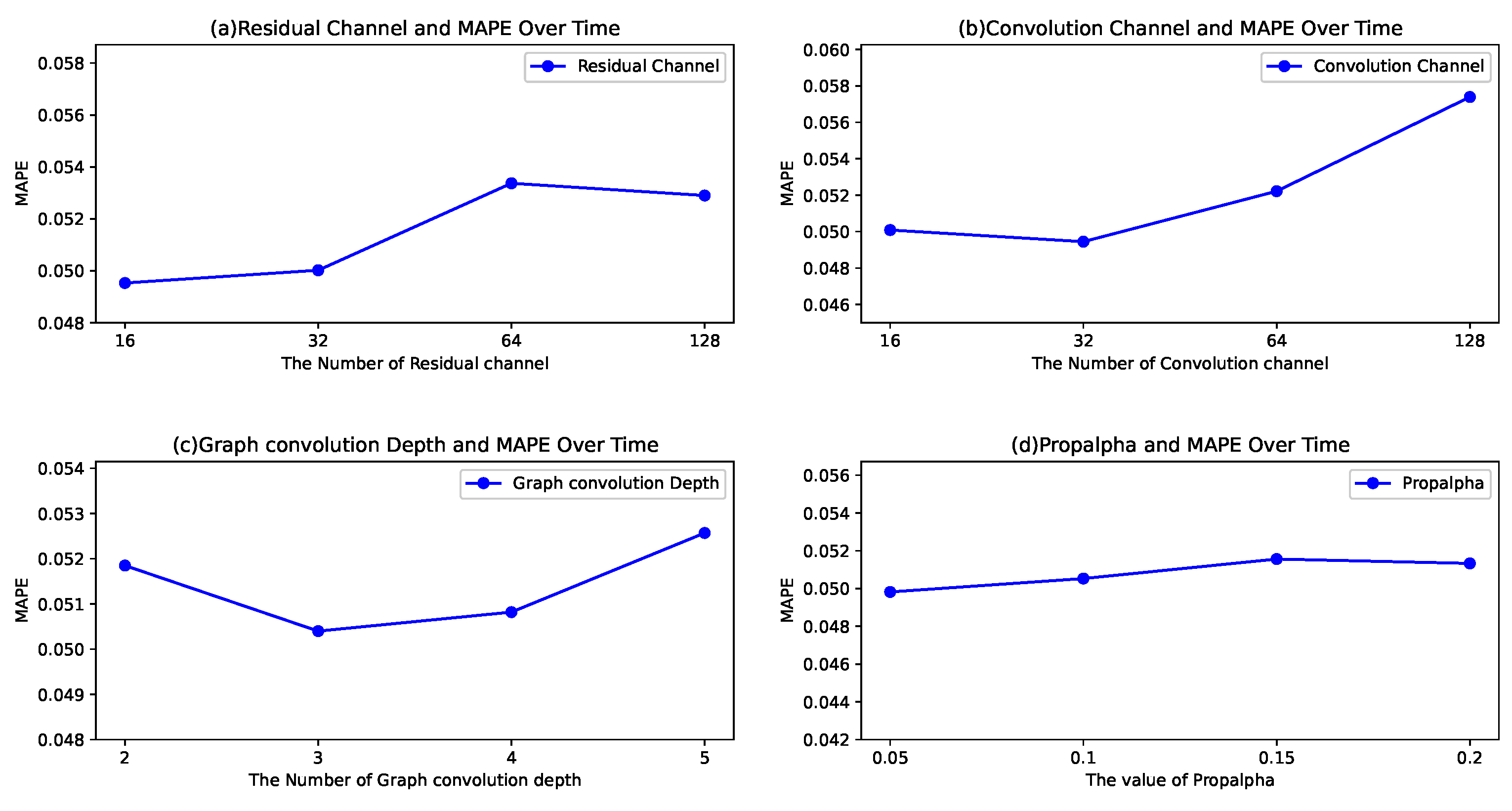
5.2. Parameter Sensitivity Analysis

We conduct a parameter study on four core hyper-parameters that influence the complexity of CIRGNN. We list these hyper-parameters as follows: residual channel, convolution channel, graph convolution depth, and $\eta$.

In each experiment, we iterate the process 10 times, with each iteration consisting of 10 epochs, and subsequently calculate the average MAPE. The parameters under investigation vary, while other parameters are constant across experiments.

The experimental results of the parameter study are shown in Figure 2. The potential improvement in prediction performance resulting from the augmentation of convolutional channels and residual connections is contingent upon the particular task, dataset, and model architecture. In general tasks, amplifying the number of convolutional channels and residual connections may bolster the model’s expressive capacity, thereby enhancing its performance; however, this augmentation carries the inherent risk of overfitting. The broken lines in Figure 2a,b indicate that, based on the dataset we collected, an optimal configuration for achieving better results is when the number of residual channels is set to 16 and the number of convolutional channels is set to 32. However, it is noteworthy that increasing the convolutional channels and residual connections escalates model complexity, which, if not carefully managed, may lead to overfitting in the stock prediction task and consequently diminish prediction accuracy. As shown in Figure 2c, the model performs the best when the convolutional depth of the graph is set to 3. This may be because a depth of 2 is too shallow to capture the complex relationships and features in the data. Conversely, when the convolutional depth exceeds 3, it becomes too deep, leading to information propagation over excessively long distances in the graph structure. This makes it difficult for the model to effectively capture the relationships between local and global features in the input. The model performance is not sensitive to the hyper-parameter $\eta$, as shown in Figure 2d, but for our model, when the $\eta$ is set to 0.05 the model has the lowest mean MAPE.

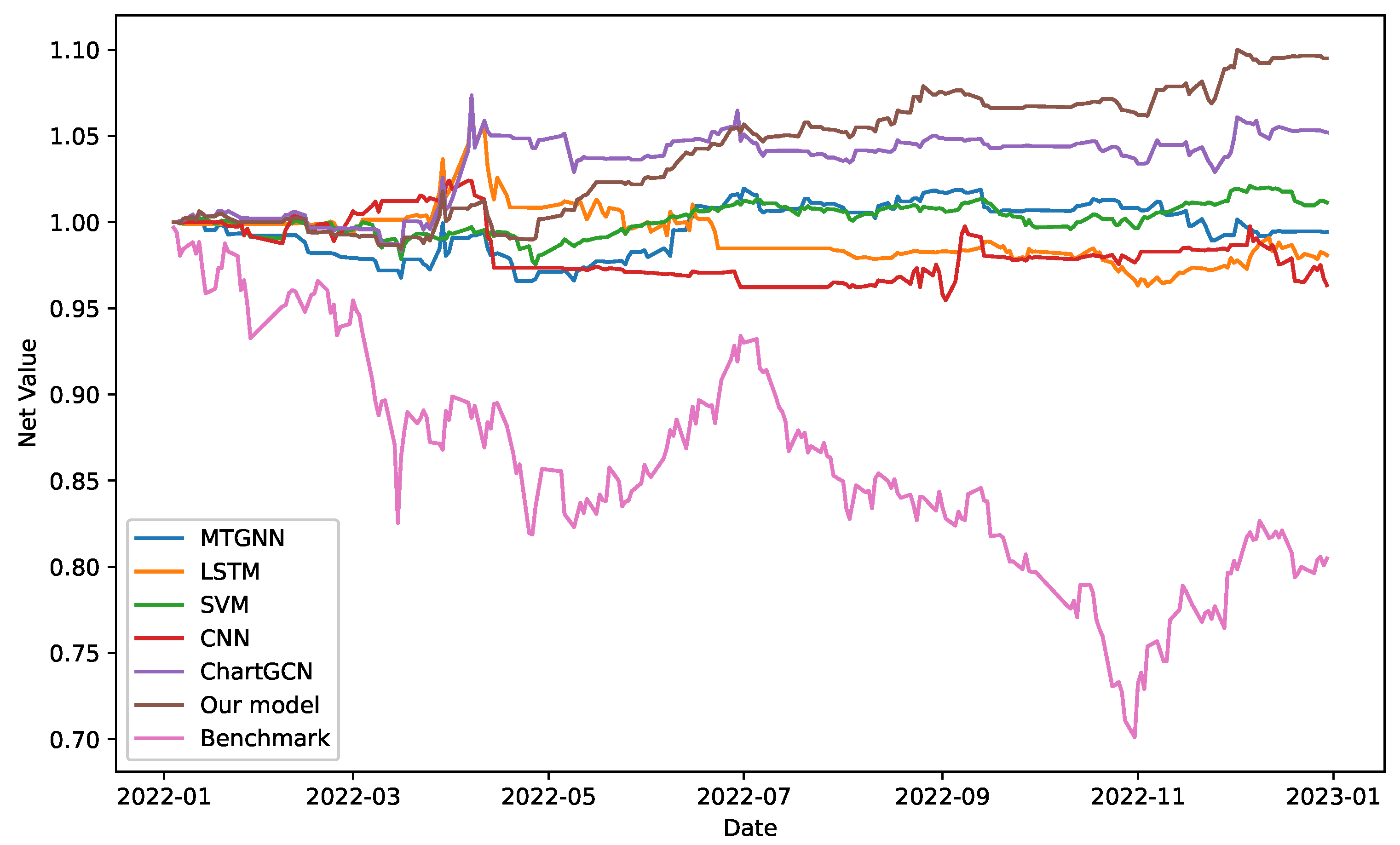
5.3. Trading Simulation

The ultimate objective of stock price prediction is to generate profits within the authentic stock market environment, necessitating the selection of test-set data, particularly from the year 2022, for conducting trading simulations.

Backtesting was performed using RQAlpha, a Python-based open-source framework developed by RiceQuant (RiceQuant: http://www.ricequant.com, accessed on 30 March 2025) for algorithmic trading and simulation. By uniformly holding each stock within the SSE 50 index as a benchmark, we compute the average return on the constituent stocks, thereby indicating the comprehensive market trend. Due to regulatory restrictions inherent in the Chinese stock market, traders are constrained to exclusively engage in long positions with stocks. The model only initiates or closes long positions based on predicted returns, fully complying with market regulations. Short-selling is neither supported nor simulated in any case.

Additionally, considering the stamp tax and stock trading fees, it is more rational to set a threshold for generating trading signals. In our backtesting, we account for practical trading frictions by including transaction costs modeled as a fixed 0.05% per trade, reflecting typical commission and stamp tax for Chinese A-shares, and by incorporating slippage as small random deviations from the predicted execution price.

Specifically, we generate the trading signals as follows: In response to long signals, contingent upon our model predicting that the subsequent day’s closing price will exceed today’s by more than $5\%$, we will hold a long position before the conclusion of the current trading day. It is crucial to emphasize that no action will be taken if a long position has already been established. Conversely, concerning short signals, should our model anticipate a decline of over $5\%$ in the following day’s closing price compared to today’s, we will sell a long position before the close of the current trading day. Nevertheless, if a short position is already established, no further action will be pursued.

The 5% gain/loss threshold was chosen to filter for high-confidence signals that are more likely to overcome normal market fluctuations and transaction costs. While not fine-tuned for optimality, this threshold reflects practical intuition: trades should only be triggered when expected gains are sufficiently large. We emphasize that this threshold is illustrative rather than prescriptive, and future work may employ adaptive or learned thresholds based on market volatility or cost constraints.

The predictive results of our model clearly demonstrate that, when combined with an appropriate trading strategy, it achieves stable and robust profitability, even in highly volatile market conditions.

The net value curves of the models during simulations are depicted in Figure 3, wherein our proposed framework demonstrates superior net asset value compared to all baseline methods, even amidst a market downturn in 2022.

A detailed, phase-by-phase analysis of the backtest results provides further insight into the model’s robustness and adaptability. Firstly, during periods of sharp market decline (e.g., January–April and July–October 2022), the model exhibited outstanding defensive strength. While the benchmark index experienced significant drawdowns, our model’s net value remained exceptionally stable, effectively insulating the portfolio from systemic risk. Secondly, the model also proved its agility in capitalizing on positive trends. It successfully participated in the mid-year rebound (May–June 2022) and further capitalized on the year-end rally (November–December 2022), ultimately reaching its annual performance peak. This consistent performance in both worst-case (decline) and best-case (rebound) phases within a volatile year underscores the practical advantage of the CIRGNN framework.

To further assess the financial utility of different models, we report a set of economic performance metrics in

Table 4. Performance metrics of backtesting.

Model	Annualized Return	Sharpe Ratio	Alpha	Beta	Max Drawdown	Information Ratio
SVM	−0.0224	−1.5315	−0.0200	0.1076	0.0280	−0.0350
LSTM	−0.0385	−0.4000	−0.0345	0.1151	0.1502	−0.1184
CNN	−0.0410	−0.3728	−0.0159	0.2089	0.1696	0.0097
MTGNN	−0.0374	−0.6151	−0.0350	0.1080	0.0749	−0.1779
ChartGCN	0.0514	0.3123	0.0654	0.1595	0.0685	0.7884
CIRGNN	0.1000	0.9647	0.1015	0.1037	0.0468	1.5757

Bold indicates the best result in column.

, including annualized return, Sharpe ratio, alpha, beta, maximum drawdown, and information ratio. As shown, CIRGNN outperforms all baselines by a significant margin across most indicators. Specifically, it achieves the highest Sharpe ratio (0.9647), alpha (0.1015), and information ratio (1.5757), indicating superior risk-adjusted returns. Moreover, CIRGNN maintains a relatively low maximum drawdown (0.0468), suggesting stronger downside protection. These results demonstrate that CIRGNN not only improves predictive accuracy but also translates into better trading performance in practical scenarios.

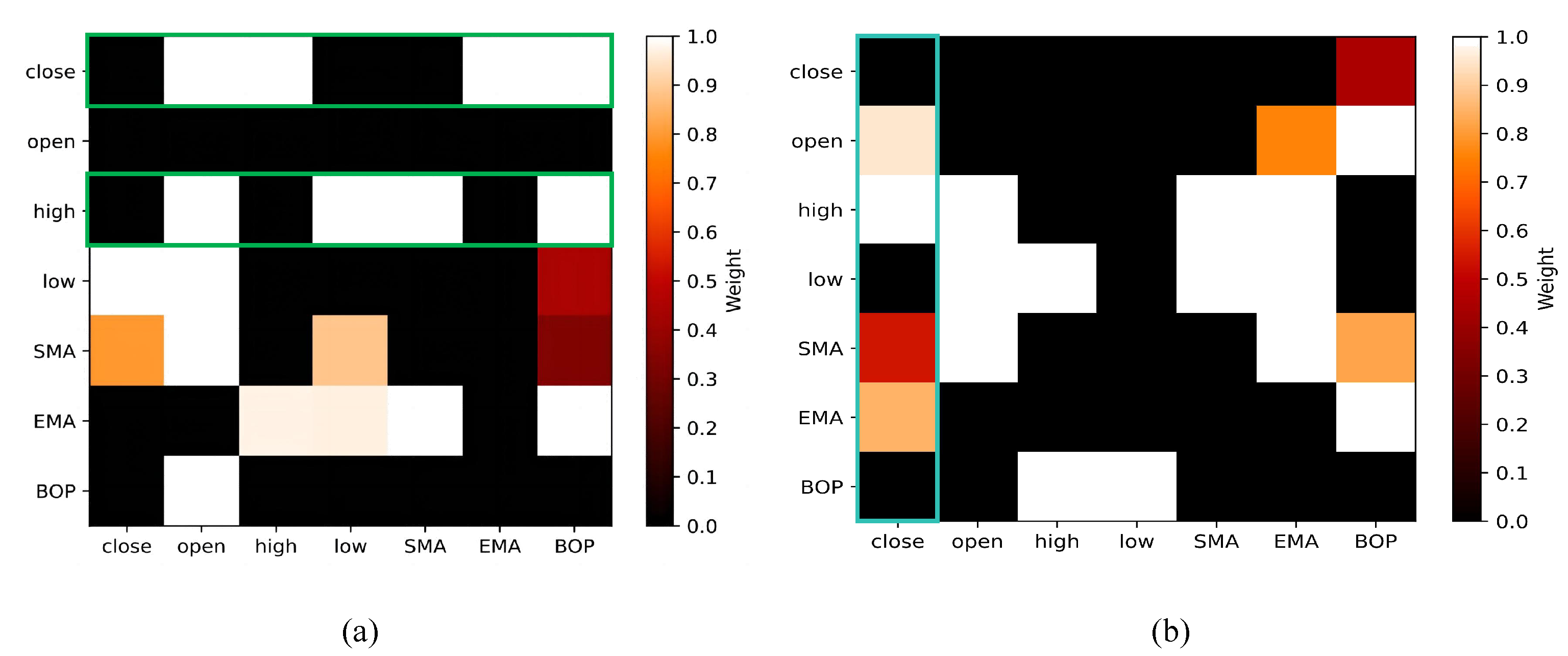
5.4. Interpretability of the Model

Although the model is trained using five technical indicators, our interpretability analysis focuses on SMA, EMA, and BOP, and also incorporates open, high, and low prices. This selection provides a clearer and more interpretable visualization of structural relationships among key features. By combining representative technical indicators with raw price components, we are able to highlight the most informative dependencies in the heatmap and provide deeper insights into how different aspects of market data interact within our model’s learned structure. The underlying VG algorithm and adaptive relationship graph learning layer allow our method to evolve and adjust these interconnections in the graph over time, enhancing the model’s ability to capture meaningful dependencies for accurate stock forecasting.

In particular, we extracted the relationship weights from the model’s learned graphs during message-passing, and visualized these as heatmaps (see Figure 4), which directly represent the cross-chart relationships adaptively learned by the model. The goal of this visualization is not to discover novel financial insights but rather to reveal how the model internally organizes and prioritizes cross-indicator relationships during prediction. This visualization reveals not only the strength but also the directionality of influences between indicators, highlighting the non-symmetric and dynamic nature of their interactions.

For example, in Figure 4a we observe that the closing price significantly affects the opening price, highest price, EMA, and BOP in some periods. The reasons may be that, firstly, a higher closing price often indicates an upward trend in the stock, potentially continuing into the next period, thus affecting subsequent opening and highest prices. Secondly, investors interpret higher closing prices as positive market sentiment, leading to buying tendencies at market open, consequently influencing opening and highest prices. Finally, higher closing prices tend to elevate EMA and bias BOP towards buying, explaining their correlations. Similarly, the highest price notably influences the opening price, lowest price, SMA, and BOP. This is due to the highest price reflecting strong demand, impacting trader sentiments and subsequent price movements [31]. Moreover, SMA calculations are sensitive to the highest price, causing shifts in trend patterns. Lastly, changes in the highest price affect traders’ sentiments, influencing the buying and selling forces reflected in the BOP indicator.

Figure 4b further illustrates how the closing price is influenced by other indicators, aligning with our study’s findings. Specifically, the opening and highest prices provide crucial market information, impacting trader decisions and subsequent price trends. Likewise, deviations in SMA and EMA signal market trends, guiding trader behavior and influencing the closing price trajectory. Interestingly, Figure 4b also indicates that the influence of the low price on the close price is relatively weak compared to other indicators. One possible explanation lies in the structural characteristics of the Chinese A-share market. Due to the inability to short-sell freely in most scenarios, investors typically do not benefit from price declines, and as a result tend to focus more on upward momentum indicators such as the open price, highest price, and moving averages (SMA, EMA), which are more directly associated with potential gains. Moreover, the low price often reflects transient dips that may be less informative for daily trading decisions, especially in a market dominated by retail investors who are more sentiment-driven and less likely to exploit intraday troughs. This asymmetry in attention may contribute to the model learning a weaker influence from the low price in predicting the close price.

To further highlight the asymmetry and directionality of these relationships, we observe that the closing price exerts strong, unidirectional influence on both EMA and BOP, while the feedback from EMA and BOP to the closing price is much weaker. This aligns with real-world financial practice: the EMA is mathematically defined as a weighted average of past closing prices, and thus always follows the closing price’s movement rather than drives it. Similarly, BOP incorporates the closing price in its computation, meaning that changes in the closing price directly affect BOP values within the same period, while BOP has minimal influence on the closing price. This asymmetric influence reflects a unidirectional dependency commonly found in the construction of technical indicators.

In another case, the highest price demonstrates a marked influence on the SMA and opening price, but not vice versa. Financially, the highest price often reflects market optimism and triggers trend-following behaviors: when a stock reaches a new high, traders may adjust their strategies, leading to higher subsequent SMA values (as the SMA calculation directly includes high points). Moreover, a sharp rise in the highest price can create bullish sentiment for the next trading day, thereby lifting the next opening price. However, the SMA or a future opening price rarely affects the current session’s highest price, highlighting the directional nature of these relationships.

These empirical findings highlight that the model not only incorporates the technical indicators but also learns their distinct predictive roles and asymmetric relationships in financial markets. Some act primarily as information sources, while others respond to or aggregate the evolving market signals. This interpretability helps confirm the effectiveness of the features and reveals how the model leverages them in a structured manner.

Although we did not perform a quantitative assessment of individual feature due to our focus on modeling interactions across technical charts, our qualitative interpretation of heatmaps provides strong evidence that each indicator plays a unique and interpretable role. Future work may incorporate feature-level analyses such as indicator dropout or SHAP-based methods to further explore model behavior.

6. Conclusions

In this paper, we present a novel framework aimed at fully leveraging the information contained within technical charts and indicators, as well as their interrelationships, for stock price prediction. Our model demonstrates enhanced robustness compared to traditional predictive models, attributable to the integration of a VG algorithm and adaptive relationship graph learning layer. By transforming technical indicator sequences into visibility graphs, our approach captures essential structural patterns that are typically leveraged by human traders but often neglected in conventional deep learning methods. Furthermore, the adaptive relationship graph learning layer dynamically models directed and asymmetric dependencies among different technical charts, allowing the framework to represent how variations in one indicator may influence others. This deeper representation of indicator interactions improves the model’s ability to understand complex market behaviors. In addition, the integration of temporal convolution and graph convolution within our architecture enables joint modeling of both temporal dynamics and the spatial relationships inherent in technical charts. This design is particularly suited to capturing the nonlinear, time-dependent, and mutually influential nature of financial time series. Our findings suggest that incorporating the relationships between technical charts derived from different indicators can contribute additional useful information for stock price prediction, compared to conventional approaches. The outstanding performance of our model in both stock price prediction and practical trading confirms the importance of technical charts, indicators, and the interrelationships of the charts in the process of stock price prediction.

Despite the valid performance demonstrated by CIRGNN, it is essential to acknowledge the presence of numerous limitations that warrant consideration and further investigation. For example, the graph returned by the graph learning layer during the process of learning the relationships between different charts remains amenable to further optimization. Additionally, we only consider the relationships between internal indicators within each stock. However, indicators of different stocks may influence one another, suggesting that exploring cross-stock indicators could improve predictive accuracy. While our current framework leverages a customized spatiotemporal GNN architecture for efficient and interpretable cross-chart modeling, future research will extend this work by investigating the integration of alternative GNN variants, such as attention-based and inductive architectures. Systematic comparison and application of these advanced models may further enhance the robustness, flexibility, and explanatory power of stock price prediction systems.

References

1. Takata, M.; Kidoguchi, N.; Chiyonobu, M. Stock recommendation methods for stability. J. Supercomput. 2024, 80, 12091–12101. [Google Scholar] [CrossRef]
2. Lee, M.C.; Chang, J.W.; Hung, J.C.; Chen, B.L. Exploring the effectiveness of deep neural networks with technical analysis applied to stock market prediction. Comput. Sci. Inf. Syst. 2021, 18, 401–418. [Google Scholar] [CrossRef]
3. Leigh, W.; Modani, N.; Purvis, R.; Roberts, T. Stock market trading rule discovery using technical charting heuristics. Expert Syst. Appl. 2002, 23, 155–159. [Google Scholar] [CrossRef]
4. Agrawal, M.; Shukla, P.K.; Nair, R.; Nayyar, A.; Masud, M. Stock Prediction Based on Technical Indicators Using Deep Learning Model. Comput. Mater. Contin. 2022, 70, 287–304. [Google Scholar] [CrossRef]
5. Tsinaslanidis, P.E. Subsequence dynamic time warping for charting: Bullish and bearish class predictions for NYSE stocks. Expert Syst. Appl. 2018, 94, 193–204. [Google Scholar] [CrossRef]
6. Wang, Y.J.; Wu, L.H.; Wu, L.C. An integrative extraction approach for index-tracking portfolio construction and forecasting under a deep learning framework. J. Supercomput. 2024, 80, 2047–2066. [Google Scholar] [CrossRef]
7. Li, S.; Wu, J.; Jiang, X.; Xu, K. Chart GCN: Learning chart information with a graph convolutional network for stock movement prediction. Knowl.-Based Syst. 2022, 248, 108842. [Google Scholar] [CrossRef]
8. Wu, J.; Xu, K.; Chen, X.; Li, S.; Zhao, J. Price graphs: Utilizing the structural information of financial time series for stock prediction. Inf. Sci. 2022, 588, 405–424. [Google Scholar] [CrossRef]
9. Dahlquist, J.R.; Kirkpatrick, C.D., II. Technical Analysis: The Complete Resource for Financial Market Technicians; FT Press: Upper Saddle River, NJ, USA, 2010. [Google Scholar]
10. Nti, I.K.; Adekoya, A.F.; Weyori, B.A. A systematic review of fundamental and technical analysis of stock market predictions. Artif. Intell. Rev. 2020, 53, 3007–3057. [Google Scholar] [CrossRef]
11. Dumiter, F.C.; Turcaș, F.M. Charts Used in Technical Analysis. In Technical Analysis Applications: A Practical and Empirical Stock Market Guide; Springer: Berlin/Heidelberg, Germany, 2023; pp. 71–89. [Google Scholar]
12. Jiang, W.; Luo, J. Graph neural network for traffic forecasting: A survey. Expert Syst. Appl. 2022, 207, 117921. [Google Scholar] [CrossRef]
13. Lacasa, L.; Luque, B.; Ballesteros, F.; Luque, J.; Nuno, J.C. From time series to complex networks: The visibility graph. Proc. Natl. Acad. Sci. USA 2008, 105, 4972–4975. [Google Scholar] [CrossRef]
14. He, Q.Q.; Siu, S.W.I.; Si, Y.W. Instance-based deep transfer learning with attention for stock movement prediction. Appl. Intell. 2023, 53, 6887–6908. [Google Scholar] [CrossRef]
15. Cervelló-Royo, R.; Guijarro, F.; Michniuk, K. Stock market trading rule based on pattern recognition and technical analysis: Forecasting the DJIA index with intraday data. Expert Syst. Appl. 2015, 42, 5963–5975. [Google Scholar] [CrossRef]
16. Tsinaslanidis, P.; Guijarro, F. What makes trading strategies based on chart pattern recognition profitable? Expert Syst. 2021, 38, e12596. [Google Scholar] [CrossRef]
17. Gilmer, J.; Schoenholz, S.S.; Riley, P.F.; Vinyals, O.; Dahl, G.E. Neural message passing for quantum chemistry. In Proceedings of the International Conference on Machine Learning, Sydney, NSW, Australia, 6–11 August 2017; PMLR: Cambridge, MA, USA, 2017; pp. 1263–1272. [Google Scholar]
18. Xiao, T.; Chen, Z.; Wang, D.; Wang, S. Learning how to propagate messages in graph neural networks. In Proceedings of the 27th ACM SIGKDD Conference on Knowledge Discovery & Data Mining, Virtual Event, 14–18 August 2021; pp. 1894–1903. [Google Scholar]
19. Liao, L.; Hu, Z.; Zheng, Y.; Bi, S.; Zou, F.; Qiu, H.; Zhang, M. An improved dynamic Chebyshev graph convolution network for traffic flow prediction with spatial-temporal attention. Appl. Intell. 2022, 52, 16104–16116. [Google Scholar] [CrossRef]
20. Han, H.; Xie, L.; Chen, S.; Xu, H. Stock trend prediction based on industry relationships driven hypergraph attention networks. Appl. Intell. 2023, 53, 29448–29464. [Google Scholar] [CrossRef]
21. Cheng, D.; Yang, F.; Xiang, S.; Liu, J. Financial time series forecasting with multi-modality graph neural network. Pattern Recognit. 2022, 121, 108218. [Google Scholar] [CrossRef]
22. Wu, Z.; Pan, S.; Long, G.; Jiang, J.; Chang, X.; Zhang, C. Connecting the dots: Multivariate time series forecasting with graph neural networks. In Proceedings of the 26th ACM SIGKDD International Conference on Knowledge Discovery & Data Mining, Virtual Event, 6–10 July 2020; pp. 753–763. [Google Scholar]
23. Zhou, J.; Cui, G.; Hu, S.; Zhang, Z.; Yang, C.; Liu, Z.; Wang, L.; Li, C.; Sun, M. Graph neural networks: A review of methods and applications. AI Open 2020, 1, 57–81. [Google Scholar] [CrossRef]
24. Wu, L.; Cui, P.; Pei, J.; Zhao, L.; Guo, X. Graph neural networks: Foundation, frontiers and applications. In Proceedings of the 28th ACM SIGKDD Conference on Knowledge Discovery and Data Mining, Washington, DC, USA, 14–18 August 2022; pp. 4840–4841. [Google Scholar]
25. Li, S.; Liu, Y.; Chen, X.; Wu, J.; Xu, K. Forecasting turning points in stock price by integrating chart similarity and multipersistence. IEEE Trans. Knowl. Data Eng. 2024, 36, 8251–8266. [Google Scholar] [CrossRef]
26. Shynkevich, Y.; McGinnity, T.M.; Coleman, S.A.; Belatreche, A.; Li, Y. Forecasting price movements using technical indicators: Investigating the impact of varying input window length. Neurocomputing 2017, 264, 71–88. [Google Scholar] [CrossRef]
27. Lin, Y.; Liu, S.; Yang, H.; Wu, H. Stock trend prediction using candlestick charting and ensemble machine learning techniques with a novelty feature engineering scheme. IEEE Access 2021, 9, 101433–101446. [Google Scholar] [CrossRef]
28. Shah, J.; Vaidya, D.; Shah, M. A comprehensive review on multiple hybrid deep learning approaches for stock prediction. Intell. Syst. Appl. 2022, 16, 200111. [Google Scholar] [CrossRef]
29. Fischer, T.; Krauss, C. Deep learning with long short-term memory networks for financial market predictions. Eur. J. Oper. Res. 2018, 270, 654–669. [Google Scholar] [CrossRef]
30. Liu, Y.; Hu, T.; Zhang, H.; Wu, H.; Wang, S.; Ma, L.; Long, M. iTransformer: Inverted Transformers Are Effective for Time Series Forecasting. In Proceedings of the Twelfth International Conference on Learning Representations, Vienna, Austria, 7–11 May 2024. [Google Scholar]
31. Kundu, R.; Chattopadhyay, S.; Nag, S.; Navarro, M.A.; Oliva, D. Prism refraction search: A novel physics-based metaheuristic algorithm. J. Supercomput. 2024, 80, 10746–10795. [Google Scholar] [CrossRef]
Figure 1. The framework of CIRGNN.
Mathematics 13 02402 g001
Figure 2. The MAPE of different parameter setting.
Mathematics 13 02402 g002
Figure 3. The backtest results.
Mathematics 13 02402 g003
Figure 4. The relationship weights of different indicators. Note: The green rectangle highlights the influence relationships where close, open, and high either act as influencing factors (rows) or as targets being influenced (columns).
Mathematics 13 02402 g004