Abstract
This paper suggests an extensive inferential method for the Power Pratibha Distribution (PPD) under Unified Hybrid Censoring Schemes (UHCSs), since there is a growing interest in flexible models in both reliability and service operations. This work studies the PPD model using standard Maximum Likelihood Estimation methods and modern Bayesian approaches too. Using a complex architecture, UHCS simulates tests more closely to what is done in practice than by using more basic censoring schemes. Using analysis, the probability and statistical ranges are carefully calculated for the parameters. Tests demonstrate that Bayesian estimation gives better results than many other methods for estimation, especially when the dataset is not very large and when a lot of data is missing. Real-world tests of electromigration failure data and banking service times help to test the methods. In both situations, the PPD shows it can be used successfully in different reliability settings. By joining advanced censoring models and reliable statistical methods, this research gives a helpful toolset to experts in reliability analysis and statistics.
Keywords:
Power Pratibha Distribution; Unified Hybrid Censoring; Bayesian estimation; maximum likelihood estimation; reliability analysis; real data application MSC:
62E10; 62F15; 62N05; 62P30; 60E05
1. Introduction
Statistical inference is very important in the analysis of lifetime data for reliability engineering, biomedical research, and service operations. Correct modeling and estimating of failures or service durations need flexible probabilities and strong estimation methods, mainly when data are censored. Sometimes, traditional censoring techniques like Type-I and Type-II are not able to include the complexities of real testing conditions. As a result, UHCS, defined by Balakrishnan et al. [1], have come to the forefront and use the best parts of each option while being more useful for practice.
It is not an easy process, theoretically, to develop unbiased inference with UHCS, mainly when the underlying distribution is complex. Although MLE is very effective, Bayesian methods are becoming more popular since they make better use of prior data and give reliable results, even when the sample size is small. For other types of lifetime distributions, making analytical calculations and obtaining accurate information from mixed-scheme estimators are currently the subjects of research.
It takes part in the ongoing dialogue by researching the PPD under different types of hybrid censorship. The PPD, defined by Prodhani1 and Shanker [2], has two adjustable parameters that help it handle a variety of risks, so it suits automotive as well as electronic industries. Even though the PPD has excellent potential, not much work has been done on using it with hybrid censoring, which this study aims to remedy.
To understand the effectiveness of the suggested inference methods, we both implement MLE and the Bayesian approach for parameter estimation in a wide range of UHCS scenarios. The simulation looks into the estimators’ performance by investigating their mean squared error, the length of the confidence intervals, and their coverage probability. In addition, the model has proven useful by analyzing real-world sets of data: (1) the durability of microelectronics and (2) the delays experienced by customers at banks. They show that the PPD is appropriate and adaptable when modeling many different types of time-to-event data.
Studies carried out lately highlight how important it is to deal with flexible distributions and consider censoring schemes in many models today. Some researchers, such as Nagy [3], Abushal [4], Balakrishnan et al. [5], and Sultan and Emam [6], are studying new mathematical life models under mixed censoring. Meanwhile, Tiefeng [7] has emphasized the key role of Bayesian methods for reliability purposes. Using what was learned from these developments, we built a strong framework that helps infer reliability and operating parameters from various data.
Some recent papers have stressed the applicability of Unified Hybrid Censoring Schemes (UHCSs) to enhance the inference of complicated lifetime models. As an illustration, Lone et al. [8] used UHCS to approximate parameters of the gamma-mixed Rayleigh distribution, showing the efficacy of the scheme in censoring scheme optimization. On the same note, Nagy and Alrasheedi [9] performed both classical and Bayesian analysis of the Pareto model under Type-II unified progressive hybrid censoring, whereas Shahrastani and Makhdoom [10] applied a unified hybrid approach to E-Bayesian inference of the inverse Weibull distribution. These investigations justify the flexibility and the inferential performance of UHCS in a diverse range of parametric lifetime models, which encourages its usage in our task to the Power Pratibha Distribution.
Simultaneously with the development of censoring schemes, substantial progress has also been achieved in federated learning (FL) predictive techniques of classifying models of the remaining useful life (RUL). It is important to note that Xu et al. [11] suggested a strategic combination of adaptive sampling and ensemble approaches in a federated platform, which led to better RUL prediction performance of aircraft engines without compromising the privacy of data.
The paper is written in seven sections to explain how parameter estimation is used in reliability studies. Section 1 starts with talking about the purpose of the study, and Section 2 examines the PPD, describes what it is, and explains its relationship with different types of failure data. It is the next section, Section 3, that presents Maximum Likelihood Estimation (MLE) to estimate the values of the model’s parameters. Bayesian estimation is introduced in Section 4, and in Section 5, the authors perform a simulation analysis to test how well the methods work in different cases. This section, Section 6, of the study shows that the approaches work well by giving examples from a real-life dataset. In the end, the authors sum up the key points from the study in Section 7.
2. Power Pratibha Distribution
This section presents the Power Pratibha Distribution, the probability distribution under the proposed study. In this section, some statistical properties of the PPD are discussed to show the importance of the PPD as a well-fitted probability model to different datasets across wide aspects of scientific applications.
Prodhani and Shanker [2] have proposed the Power Pratibha Distribution (PPD), a flexible two-parameter model obtained as a power transformation of the Pratibha distribution. PPD overcomes the deficiencies of one-parameter lifetime models because it improves fits to complex data.
A random variable X is said to have a PPD iff its Probability Density Function (PDF) is given by:
The Cumulative Distribution Function (CDF) of the PPD can be written as
Meanwhile, the survival function of PPD is as follows:
Prodhani and Shanker [2] have shown that the PPD offers greater flexibility, fits real-world lifetime data better than competing models, and possesses strong reliability characteristics. It has well-defined statistical measures like moments, coefficient of variation, and dispersion index. Also, they have illustrated that PPD allows different patterns of skewness and hazard rates, such as decreasing and bathtub. Prodhani and Shanker [2] have estimated the parameters of PPD for complete data and have not considered any censoring scheme. However, our contribution generalizes the analysis to consider UHCS, which is more flexible to the tested data that, in practice, is partially observed because of time or resource constraints.
Figure 1, Figure 2 and Figure 3 illustrate that the PPD is flexible in fitting a wide variety of hazard rate behaviors. By varying parameters, and , it can capture increasing, decreasing, and bathtub-shaped hazard functions, and hence can be used in a large number of reliability applications.
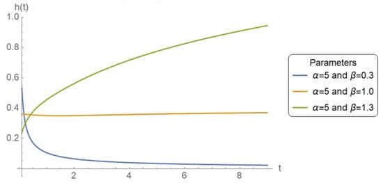
Figure 1.
Effect of on for
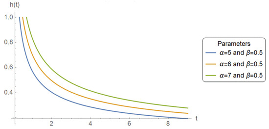
Figure 2.
Effect of on when
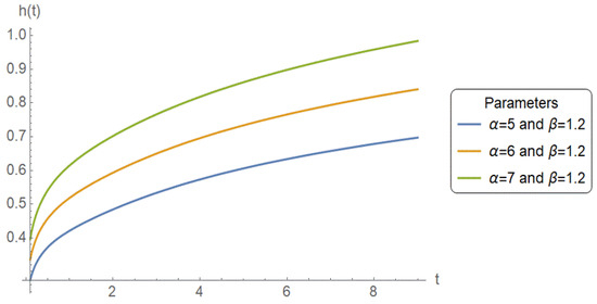
Figure 3.
Effect of on when
3. Maximum Likelihood Estimation
To find out the best parameter values for the data, the likelihood function is used, and so it is vital in statistical inference. It is used to estimate parameters (for example, in Maximum Likelihood Estimation) and to make confidence intervals and hypothesis tests. In general, it links the data to the model parameters and leads us to understand the unknowns.
The likelihood function given by Balakrishnan et al. [1] based on UHCS can be written as follows:
The datasets here, , are UHCS, which are observed according to the manner presented by Balakrishnan et al. [1]. According to UHCS, two pre-fixed termination times, and for a lifetime experiment have been assigned, where and denote the number of observed failure units before and respectively. The lifetime experiment may be terminated at or where as n is the number of the tested units involved in the lifetime experiment. The UHCS is defined to guarantee obtaining at least k observed units and, hence, to obtain good inferential results.
The likelihood function can be displayed in a brief presentation as follows:
where H and may take one of the following values as per the corresponding unified hybrid schemes:
| Scheme | H | ||
| 1st | D | ||
| 2nd | r | ||
| 3rd | |||
| 4th | r | ||
| 5th | |||
| 6th | k | ||
Therefore, the log-likelihood function, denoted by data takes the following form:
By plugging in the PDF and CDF of the PPD from Equations (1) and (2), respectively, into Equation (6), the partial derivatives of the with respect to the parameters and can be derived as follows:
Equations (7) and (8) are nonlinear simultaneous equations in the unknown variables and . It is clear that an exact solution is difficult to be obtained. Therefore, a numerical approach such as Newton Raphson can be used to obtain the approximate solution. The steps of Newton Raphson algorithm is described in details in Casella and Berger [12]. The final solution of this nonlinear simultaneous equations are the MLEs of the parameters and , denoted as and . Mathematica software, version 12, has been used to apply the Newton Raphson algorithm via a command called FindRoot, more details about this command are available via the following URL: https://reference.wolfram.com/language/ref/FindRoot.html, accessed on 1 June 2025. The second partial derivatives of the log-likelihood functions are derived as follows:
Moreover, using the invariance property of MLEs, the MLEs of and can be obtained after replacing and by and as
Both functions are completely parameterized with MLEs and can thus be usefully applied in the estimation with real data. Such expressions play a key role in assessing the reliability of systems, forecasting failures, and forming confidence intervals to use in operation decisions.
Approximate Confidence Intervals
The asymptotic variances and covariances of the MLEs, and are given by the entries of the inverse of the Fisher information matrix , where and Unfortunately, the exact closed forms for the above expectations are difficult to obtain. Therefore, the observed Fisher information matrix which is obtained by dropping the expectation operator E, will be used to construct confidence intervals for the parameters. The observed Fisher information matrix has second partial derivatives of log-likelihood function as the entries, which easily can be obtained. Hence, the observed information matrix is given by
Therefore, the approximate (or observed) asymptotic variance-covariance matrix for the MLEs is obtained by inverting the observed information matrix or the following equivalent:
It is well known that under some regularity conditions, (see Lawless [13]), MLEs of is approximately distributed as multivariate normal with mean and covariance matrix . Then, the two-sided confidence intervals of and , can be given by
where is the percentile of the standard normal distribution with right-tail probability .
Furthermore, to construct the asymptotic confidence interval (ACI) of the reliability and hazard functions, which they are functions in the parameters and , the variance of these two functions should be estimated. In order to find the approximate estimates of the variance of and , we use the delta method. The delta method is a general approach for computing CIs for functions of MLEs, see Greene [14]. According to this method, the variance of and can be approximated, respectively, by
where and are, respectively, the gradient of and with respect to and
The quantities, and are computed as follows:
while
and
Then, the two-sided confidence intervals of and can be given by
These two intervals to and give an asymptotic measure of uncertainty, via the delta method, with standard normal quantiles. They are required to estimate both reliability and risk at any given time point, and in particular, moderate and large samples.
4. Bayesian Estimation
Bayesian estimation relies on both previous understanding and new data to improve ideas and take decisions. It uses Bayes’ theorem to change the probability distribution of the parameter after gathering data. This way of doing inference differs from classical methods since it examines parameters as random variables with their own variability. It is especially helpful when you have prior knowledge or complicated situations, which explains why it is important in machine learning, statistics, and modeling.
The prior knowledge about the parameters of the PPD, and , can be modeled as follows:
and
The joint posterior density function of and denoted by data) can be written as
where is the joint prior distribution of and
If is the parameter to be estimated by an estimator then the squared error loss (SEL) function is defined as
and the Bayes estimate of any function of and say under the SEL function is
where
Now the joint posterior distribution , given in Equation (18), can be rewritten as follows:
The following relation gives the conditional posterior distribution of the parameter as follows:
while the following relation gives the conditional posterior distribution of the parameter as follows:
To find the Bayesian estimates for the parameters and under the SEL function, one may use Equations (20) and (21). Unfortunately, the joint posterior distribution, Equation (21), or even the conditional posteriors Equations (22) and (23) are given in a complicated formula, which makes getting an analytical solution impossible. Alternatively, the Markov Chain Monte Carlo (MCMC) method is used based on Metropolis–Hasting (M-H) approach, for more details see Mahmoud et al. [15].
The algorithm of applying the MCMC method, to obtain the Bayesian point estimates and the credible intervals CRIs for the parameters , the survival and hazard functions, is described in detail by Mahmoud et al. [15].
5. Simulation Study
To compare the estimates of parameters of the PPD, a simulation study is performed based on 1000 unified hybrid censored samples. The samples are generated from PPD using Mathematica software version 12. The command that has been used for generating the samples is Probaility Distribution. The description of this command is available via the following URL:
https://reference.wolfram.com/language/ref/ProbabilityDistribution.html, accessed on 1 June 2025. To generate the samples, some values have been chosen randomly for the parameters and , say and The simulation study is conducted at different UHCS for the values of and to conclude the best scheme for obtaining good inferential results. The comparison between the different methods of the resulting estimates has been considered in their biasness (Bias) and mean square error (MSE) which are computed, as follows:
where is the number of simulated samples.
Another criterion is used to compare the confidence intervals (CIs), at two confidence levels specifically at and , obtained by using the asymptotic distributions of the MLEs and credible intervals (CRIs). The comparison of them is made in terms of the average confidence interval lengths (ACILs) and coverage probability (CP). The CP of a confidence interval is the proportion of the time that the interval contains the initial value of interest. In the case of Bayesian approach, the hyperparameters for the informative priors, are chosen as follows: . The results of MSE biasness of the estimated parameters are shown in Table 1 and Table 2, while the results of ACIL and CPs are displayed in Table 3 and Table 4. The ACIL and CPs of both survival and hazard functions are displayed in Table 5 and Table 6.

Table 1.
Estimates for the parameter .
Table 2.
Estimates for the parameter .
Table 3.
ACILs and CPs for the parameter .
Table 4.
ACILs and CPs for the parameter .
Table 5.
ACILs and CPs for the S at
Table 6.
ACILs and CPs for the h at
Figure 4 and Figure 5 show that the distribution of estimates based on 1000 simulations is very narrow and concentrated, which shows that Bayesian estimates of and are consistent.
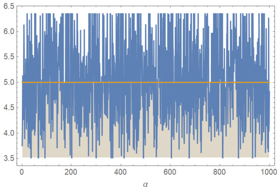
Figure 4.
Bayesian estimates for the parameter based on 1000 UHCS.
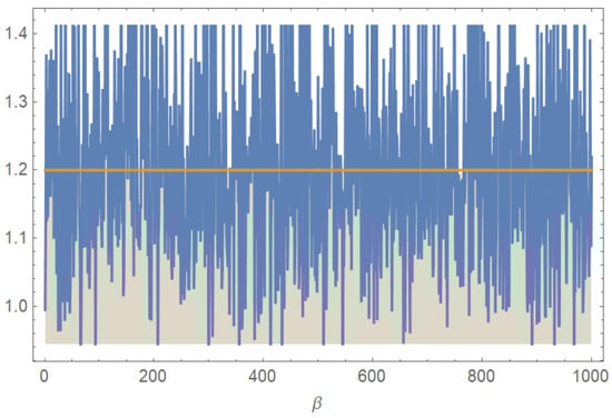
Figure 5.
Bayesian estimates for the parameter based on 1000 UHCS.
From the simulation study, it is noted that the following:
- For the parameter :
The Bayesian method consistently outperformed MLE in terms of lower bias and MSE, particularly under heavy censoring conditions (small values of ) and larger gap between k and In most cases, the Bayesian MSE indicate greater stability and robustness of the Bayesian approach.
- For the parameter :
The differences in bias and MSE between MLE and Bayesian estimation were narrower than for but the Bayesian estimates still tended to be more accurate overall. Bayesian estimates for remained relatively unaffected by variations in censoring parameters, showcasing their insensitivity to censoring complexity.
- ACIL and CPs
Bayesian intervals were consistently much shorter than their MLE counterparts across all censoring schemes, reflecting the precision of Bayesian posterior distributions. MLE-based confidence intervals generally achieved their intended coverage levels or consistent with frequentist theory. In contrast, Bayesian credible intervals, especially for parameter showed much lower coverage (often 7–17% at level), rarely exceeding even at . This undercoverage is due to the narrower interval widths in Bayesian methods, which, while more precise, are more likely to miss the true parameter particularly when priors are vague.
- and CIs
As expected, confidence intervals were slightly wider than for both methods. MLE showed a clear improvement in coverage, reinforcing its reliability. However, Bayesian intervals showed only a small increase in coverage, indicating potential underestimation of uncertainty. Notably, Bayesian intervals for had better coverage than for
6. Applications
To demonstrate the practical utility of the proposed Unified Hybrid Censoring Scheme and the flexibility of the PPD, this section presents two real-life applications. These datasets stem from reliability engineering and service operations, two domains where modeling time-to-event data is crucial. Two real datasets are analyzed to show the flexibility of the Power Pratibha Distribution: one from electromigration failure data in microelectronics and another from customer waiting times in banking. These examples illustrate the model’s effectiveness in both high-reliability and high-turnover contexts.
In both cases, we estimate the model parameters using Maximum Likelihood and Bayesian approaches, and evaluate the survival and hazard functions at selected time points. Goodness-of-fit is assessed using the Kolmogorov–Smirnov (K-S) statistic.
6.1. Electromigration Failure Data
Electromigration is a physical failure mechanism in microelectronic conductors, where high current density causes metal atoms (like aluminium or copper) in a wire to migrate. Over time, this creates breaks or bumps in the conductor. This leads to open circuits or shorts, causing the device to fail. The dataset refers to the time to failure (in hours) of 400 µm electromigration specimens; this is referred to as electromigration analyzed previously by Gamze et al. [16].
The Kolmogorov–Smirnov (K-S)distance between the empirical distribution of failure data and CDF of PPD is with p-value equals Hence, the PPD fits well to the given data.
The visual evidence that the PPD fitted the electromigration failure data is very convincing, as seen in Figure 6 and Figure 7. The p-value and near-perfect Q-Q fit show the overall distribution of the data.
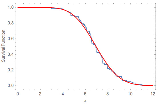
Figure 6.
K-S test for the observed data.
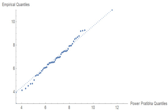
Figure 7.
Q-Q plot for the observed data.
Table 7 gives the comparative goodness-of-fit statistics of some lifetime distributions fitted to electromigration failure data. As measures of evaluation, there are Akaike Information Criterion (AIC), Bayesian Information Criterion (BIC), Hannan–Quinn Information Criterion (HQIC), and Kolmogorov–Smirnov (K-S) test p-value. The criteria have given quantitative indications that the PPD better fits the underlying observed data.
Table 7.
Goodness-of-fit results for the observed data.
In particular, 400 μm (μm) test conductors, like those in the dataset, are representative of metal lines used in microchips, printed circuit boards (PCBs), and power electronics, where high current densities cause electromigration failures. These structures are critical in devices such as processors, automotive electronic control units (ECUs), and radio frequency (RF) modules, making reliability testing essential.
The values of are chosen randomly to be , respectively, while the values of were, respectively. This choice of and r leads to applying the fourth scheme of the UHCS. At h, the estimated survival probability is approximately , meaning that nearly of the specimens are expected to still be functioning beyond this point. The hazard rate is about , indicating a low instantaneous failure risk at exactly 4 h. The narrow confidence intervals around both estimates reflect strong statistical reliability. These results suggest that early-life failures due to electromigration are rare. Overall, the Power Pratibha Distribution provides a good fit for modeling this high-reliability behavior.
6.2. Waiting Time Banking Data
Estimating both the survival function and the hazard function for waiting time data complementary insights that are highly valuable in practical applications, especially in queue management, service operations, and customer experience optimization.
The following dataset, discussed by Prodhani and Shanker [2], is obtained from the banking sector and discusses the waiting time (in minutes) before the customer received service in a bank. The values are as follows:
Based on the displayed dataset, Prodhani and Shanker [2] have compared the PPD with some lifetime distributions, such as power Lindley (PLD), power Aradhana (PAD), power Akash (PAkD), and Weibull (WD) distributions. The comparison is made using some statistical standards, including AIC, BIC, and HQIC, and the Kolmogorov–Smirnov (K-S) test. PPD has demonstrated minimal values in all these criteria compared to other models. The goodness of fit is also strong, as indicated by the K-S statistic and the high p-value for PPD. This supports the conclusion that PPD is the best model for the analyzed dataset.
The values of are chosen randomly to be , respectively, while the values of were respectively. Based on the candidate values for and r, the sixth scheme of the UHCS has been applied. The survival function gives the probability that a customer’s waiting time exceeds Therefore, implies that customers are still waiting at 2 min and only have been served by then. The corresponding hazard rate provides the instantaneous chance of service at that time. Taken together, these values indicate a relatively slower service process, with most customers experiencing waiting times beyond 2 min. It is true that these measures are useful in the diagnosis of system performance and areas in which operations can be improved.
Figure 8 and Figure 9 indicate that PPD is very effective in customer waiting time modeling. The p-value is very high, and the Q-Q alignment is excellent, indicating that the PPD is an acceptable fit to the data and thus can be used to analyze service times and make operational decisions.
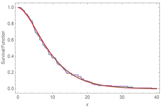
Figure 8.
K-S test for the observed data.
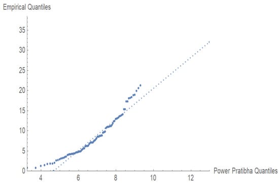
Figure 9.
Q-Q plot for the waiting time data.
The results, displayed in Table 8 and Table 9, highlight the adequacy of the PPD in fitting real data and reinforce the practical relevance of the proposed censoring and estimation strategies.
Table 8.
Inferential results for the parameters and for the survival and hazard functions at
Table 9.
Inferential results for the parameters and for the survival and hazard functions at
7. Conclusions
The paper studied the UHCS with the PPD, using both MLE and Bayesian estimation methods. The simulation study has shown that Bayesian estimation under UHCS offers superior accuracy, precision, and stability, especially with small samples or heavy censoring. However, it comes with lower coverage probabilities. MLE remains a dependable choice when reliable confidence intervals are essential. Together, both methods form a strong toolkit for analyzing complex lifetime data across various applied fields. Based on results from electromigration and banking datasets, Bayesian methods are recommended for practical applications. Moving forward, a promising development for future studies is the application of deep learning methods in reliability analysis, which is a rapidly growing field that can model dysfunctional processes in a high-dimensional. Methods, such as Bayesian deep learning or deep learning survival models, have demonstrated effectiveness when analyzing censored and complex data involving lifetimes. Also, one possibility is to integrate or align UHCS with data-centered models, including federated learning or ensemble deep models, to further improve inference results.
Author Contributions
Conceptualization, K.S.S.; Methodology, K.S.S. and M.M.M.M.; Software, M.M.M.M.; Validation, H.H.M.; Investigation, H.H.M. and K.S.S.; Data curation, M.M.M.M.; Writing—original draft, M.M.M.M.; Writing—review & editing, H.H.M. and K.S.S.; Visualization, M.M.M.M.; Supervision, K.S.S.; Funding acquisition, H.H.M. All authors have read and agreed to the published version of the manuscript.
Funding
This research project was funded by Princess Nourah bint Abdulrahman University Researchers Supporting Project number (PNURSP2025R745), Princess Nourah bint Abdulrahman University, Riyadh, Saudi Arabia.
Data Availability Statement
Data are contained within the article.
Acknowledgments
The authors acknowledge that this research project was funded by Princess Nourah bint Abdulrahman University Researchers Supporting Project number (PNURSP2025R745), Princess Nourah bint Abdulrahman University, Riyadh, Saudi Arabia.
Conflicts of Interest
The authors declare no conflicts of interest.
References
- Balakrishnan, N.; Rasouli, A.; Farsipour, N.S. Exact Likelihood Inference Based on an Unified Hybrid Censored Sample from the Exponential Distribution. J. Stat. Comput. Simul. 2008, 78, 475–488. [Google Scholar] [CrossRef]
- Prodhani, H.R.; Shanker, R. Power Pratibha Distribution with Properties and Applications. Int. J. Stat. Reliab. Eng. 2024, 11, 217–226. [Google Scholar]
- Nagy, M. Statistical Inference for Kumaraswamy Distribution under Generalized Progressive Hybrid Censoring Scheme with Application. Comput. Model. Eng. Sci. 2025, 143, 185–223. [Google Scholar] [CrossRef]
- Abushal, T.A. Statistical Inference for Nadarajah-Haghighi Distribution under Unified Hybrid Censored Competing Risks Data. Heliyon 2024, 10, e26794. [Google Scholar] [CrossRef] [PubMed]
- Balakrishnan, N.; Cramer, E.; Kundu, D. Chapter 7—Progressive Hybrid Censored Data. In Hybrid Censoring Know-How; Balakrishnan, N., Cramer, E., Kundu, D., Eds.; Academic Press: Cambridge, MA, USA, 2023; pp. 207–250. [Google Scholar] [CrossRef]
- Sultan, K.S.; Emam, W. The Combined-Unified Hybrid Censored Samples from Pareto Distribution: Estimation and Properties. Appl. Sci. 2021, 11, 6000. [Google Scholar] [CrossRef]
- Zhu, T. Reliability Inference for Multicomponent Stress–Strength Model under Generalized Progressive Hybrid Censoring. J. Comput. Appl. Math. 2024, 451, 116015. [Google Scholar] [CrossRef]
- Lone, S.A.; Panahi, H.; Anwar, S.; Shahab, S. Estimations and optimal censoring schemes for the unified progressive hybrid gamma-mixed Rayleigh distribution. Electron. Res. Arch. 2023, 31, 5066–5088. [Google Scholar] [CrossRef]
- Nagy, M.; Alrasheedi, A.F. Classical and Bayesian inference using Type-II unified progressive hybrid censored samples for Pareto model. Appl. Bionics Biomech. 2022, 2022, 2073067. [Google Scholar] [CrossRef] [PubMed]
- Shahrastani, S.Y.; Makhdoom, I. Estimating E-Bayesian of parameters of inverse Weibull distribution using a unified hybrid censoring scheme. Pak. J. Stat. Oper. Res. 2021, 17, 113–122. [Google Scholar] [CrossRef]
- Xu, A.; Wang, R.; Weng, X.; Wu, Q.; Zhuang, L. Strategic integration of adaptive sampling and ensemble techniques in federated learning for aircraft engine remaining useful life prediction. Appl. Soft Comput. 2025, 175, 113067. [Google Scholar] [CrossRef]
- Casella, G.; Berger, R.L. Statistical Inference, 2nd ed.; Duxbury Press: Pacific Grove, CA, USA, 2022. [Google Scholar]
- Lawless, J.F. Statistical Models and Methods for Lifetime Data; John Wiley and Sons: New York, NY, USA, 1982. [Google Scholar]
- Greene, W.H. Econometric Analysis, 4th ed.; Prentice-Hall: NewYork, NY, USA, 2000. [Google Scholar]
- Mahmoud, M.A.W.; Ramadan, D.A.; Mansour, M.M.M. Estimation of lifetime parameters of the modified extended exponential distribution with application to a mechanical model. Commun. Stat. Simul. Comput. 2020, 51, 7005–7018. [Google Scholar] [CrossRef]
- Ozel, G.; Alizadeh, M.; Cakmakyapan, S.; Hamedani, G.G.; Ortega, E.M.M.; Cancho, V.G. The odd log-logistic Lindley Poisson model for lifetime data. Commun. Stat. Simul. Comput. 2017, 46, 6513–6537. [Google Scholar] [CrossRef]
Disclaimer/Publisher’s Note: The statements, opinions and data contained in all publications are solely those of the individual author(s) and contributor(s) and not of MDPI and/or the editor(s). MDPI and/or the editor(s) disclaim responsibility for any injury to people or property resulting from any ideas, methods, instructions or products referred to in the content. |
© 2025 by the authors. Licensee MDPI, Basel, Switzerland. This article is an open access article distributed under the terms and conditions of the Creative Commons Attribution (CC BY) license (https://creativecommons.org/licenses/by/4.0/).