
Physical–Mathematical Modeling and Simulations for a Feasible Oscillating Water Column Plant


Abstract
1. Introduction
- Sea waves possess the highest energy density among all renewable energy sources [5]. The waves are generated indirectly by solar energy through the winds: the typical intensity of solar energy is 0.1–0.3 kW per m2 of horizontal surface, and it is converted into a concentrated and relevant wave energy flux. For example, considering a significant wave height (i.e., the average height of the highest third of the waves) of 1 m and a wave energy period of 4.5 s, we obtain a wave energy flux of 2.25 kW per meter of wave crest, which rises to 13 kW/m if m and s [6].
- Minimal environmental impact during operation. In [4] the potential impact and an estimate of the life cycle emissions of a typical nearshore device is analyzed. In general, offshore devices have the least potential impact.
- The natural seasonal variability of wave energy aligns well with electricity demand in temperate climates in a very efficient way [5].
- Waves can propagate over long distances with minimal energy loss.
- Studies have shown that wave energy converters can capture up to of available energy, compared to 20–30% for wind and solar devices [7].
Structure and Goals of the Paper
2. OWC Systems for Converting Ocean Energy
2.1. OWC: Operation, Scale Trials, and Plants Around the World
2.1.1. Considerations on OWC Operation and Physical Resonance
- the geometry and dimensions of the chamber;
- the volume of air it contains;
- the damping effect introduced by the turbine.
2.1.2. Working OWC Plants, Past and Ongoing Trials
2.2. Power Take-Off Devices Applicable to OWC Systems
- -
- conventional turbines with suitable flow rectification systems using non-return valves and auxiliary channels;
- -
- self-rectifying turbines, mainly including the Wells turbine in its various versions;
- -
- the action turbines with two distributors;
- -
- some special turbines including a Savonius rotor and Denniss–Auld turbine.
3. From Mathematical Modeling to the Definition of Plant Specifications
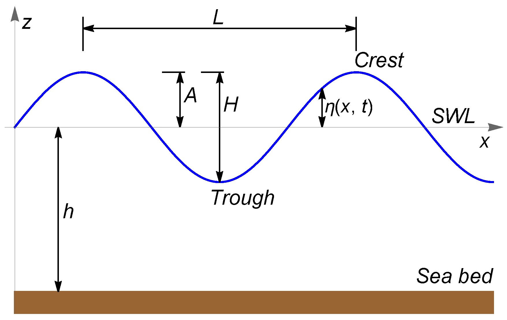
3.1. The Mathematical Modeling of Wave Motion
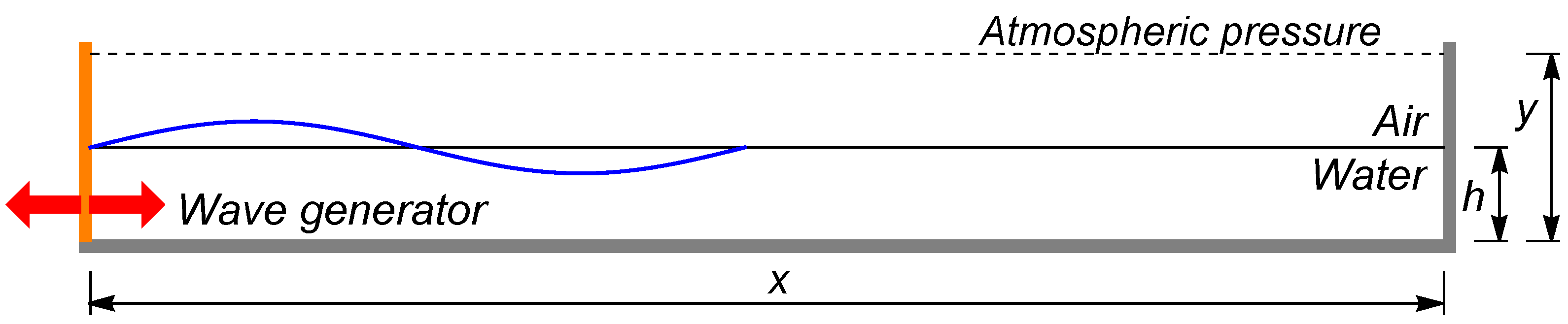
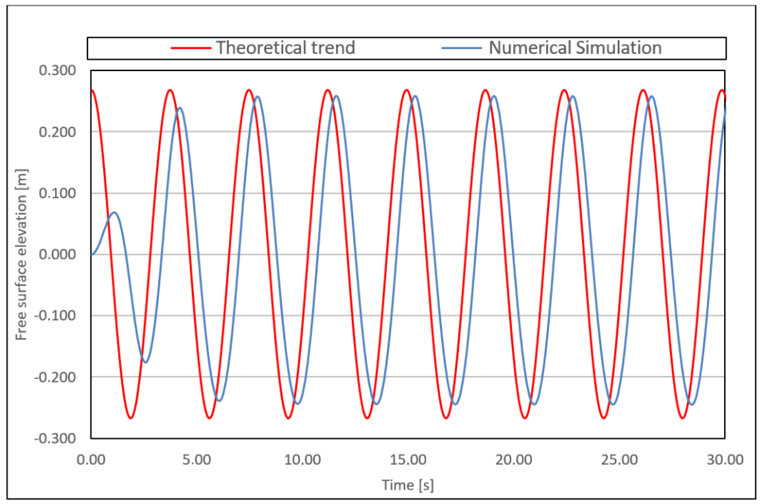
3.2. Numerical Simulation of an Induced Wave Motion
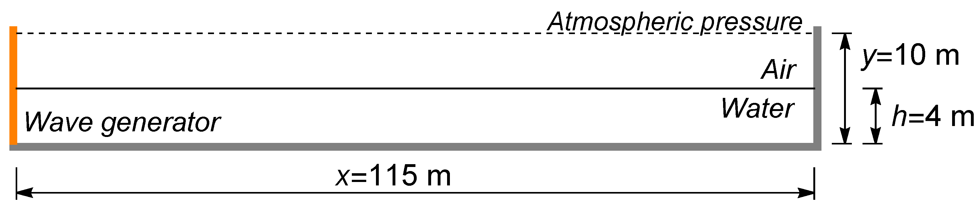
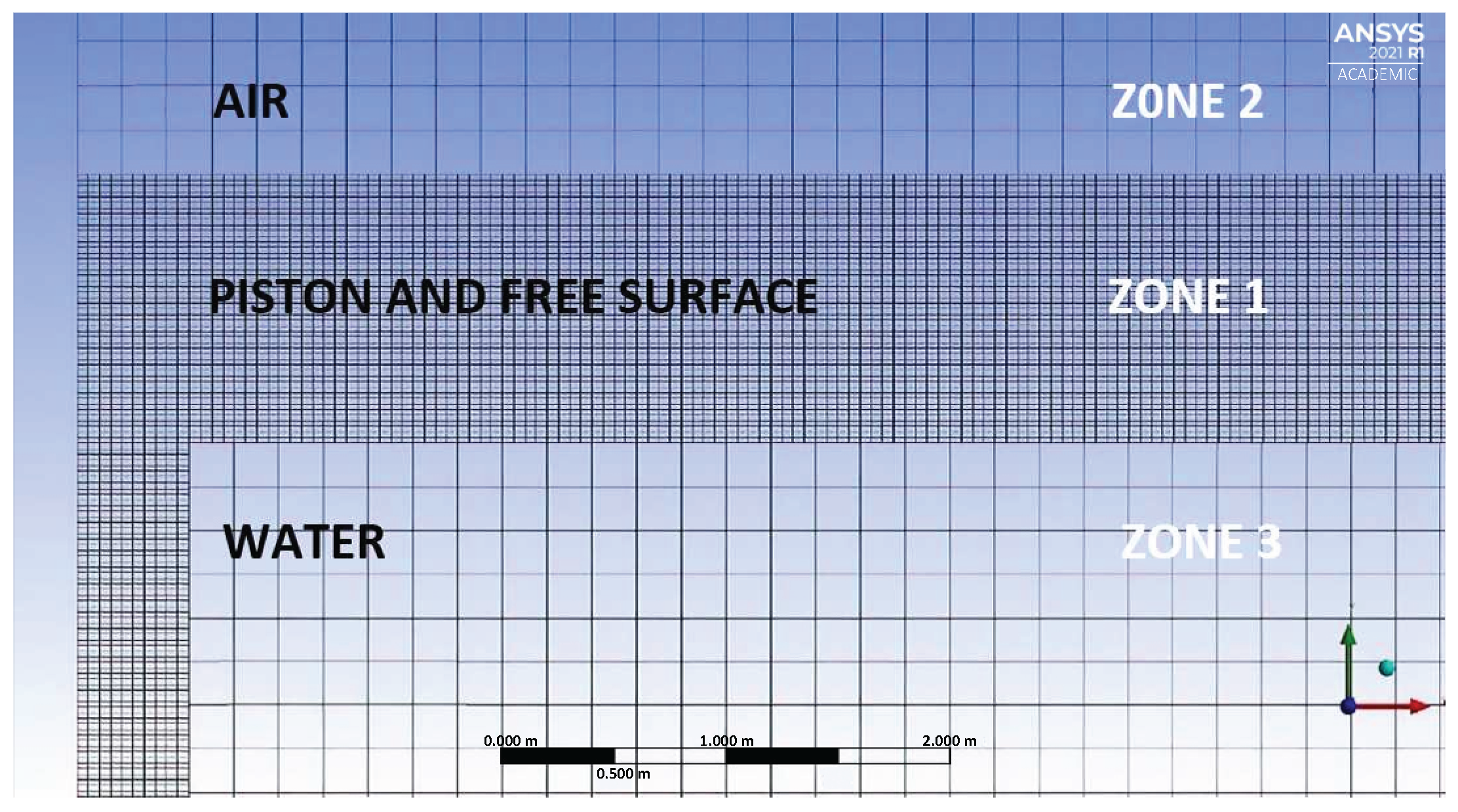
3.2.1. Definition of the Domain and of the Calculation Grid
3.2.2. Numerical Simulation Settings
- the conservation of mass (or continuity) equationwhich holds for both compressible and incompressible flows;
- the momentum balance equationwhere p is the pressure, is a source term (for example, related to a porous medium) and is the stress tensor equal towhere is the molecular viscosity;
- the energy conservation equationwhere e is the specific energy, the thermal conductivity, T the temperature, and a possible heat source.
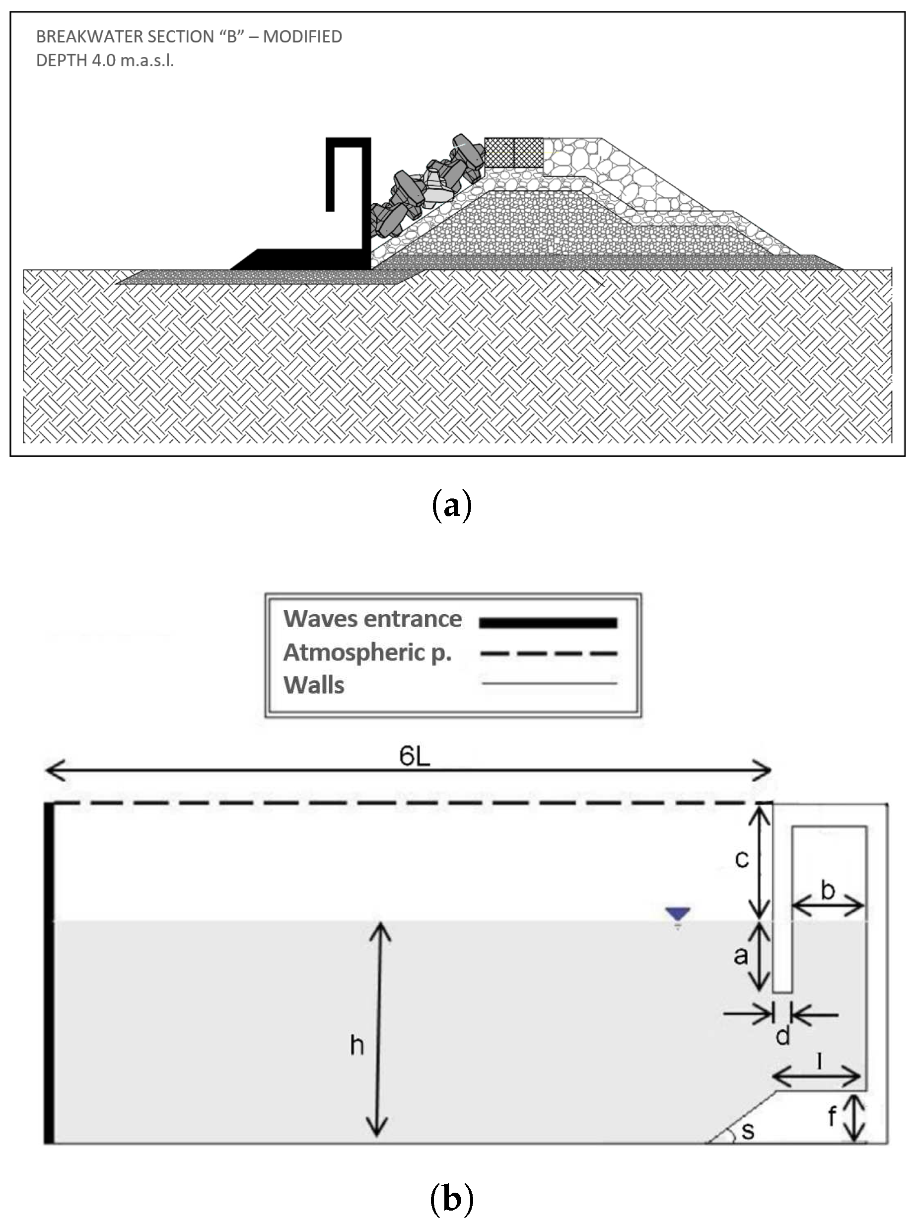
3.3. OWC Plant Specifications
4. Mathematical Modeling of the PTO and Simulation Results
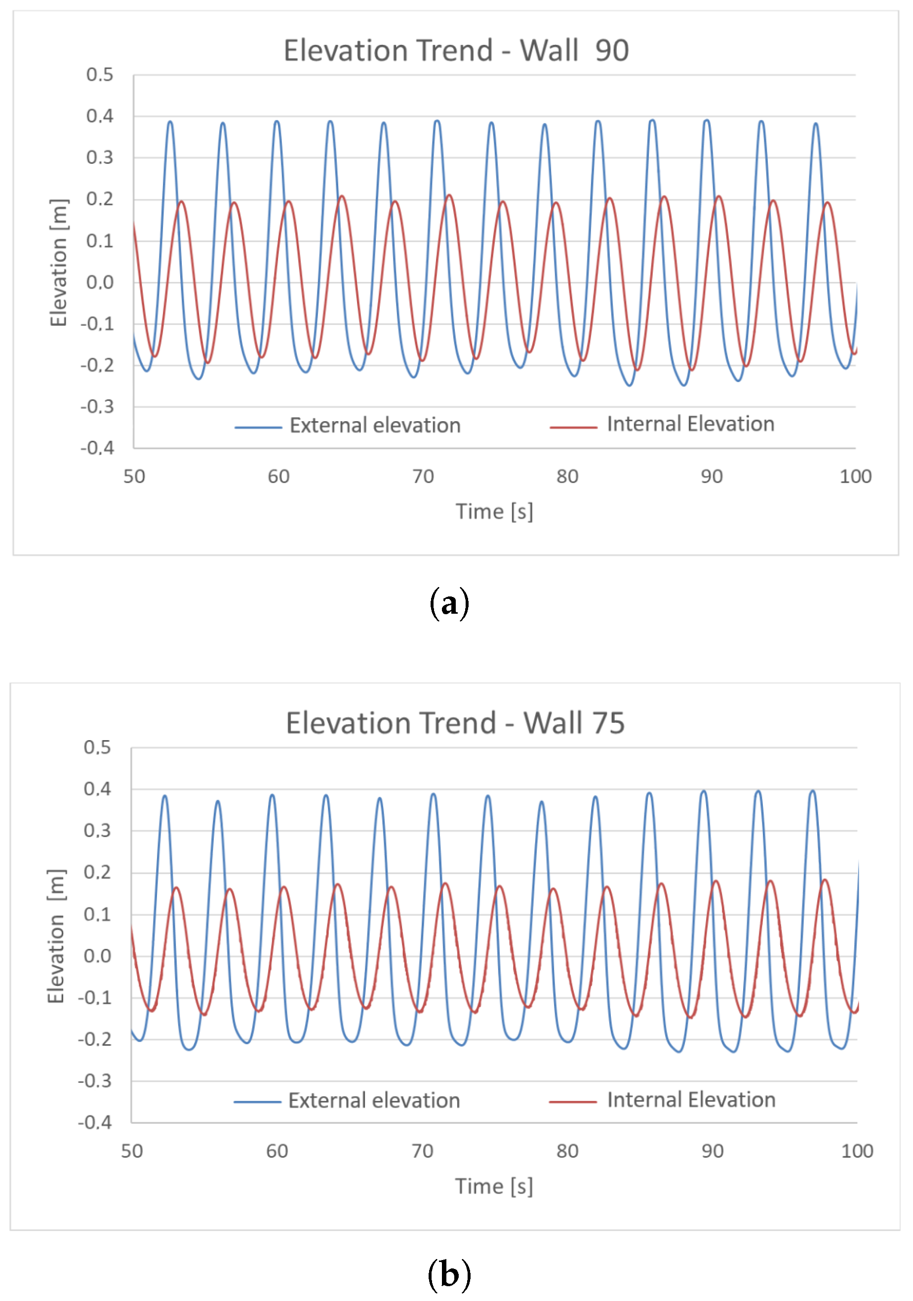
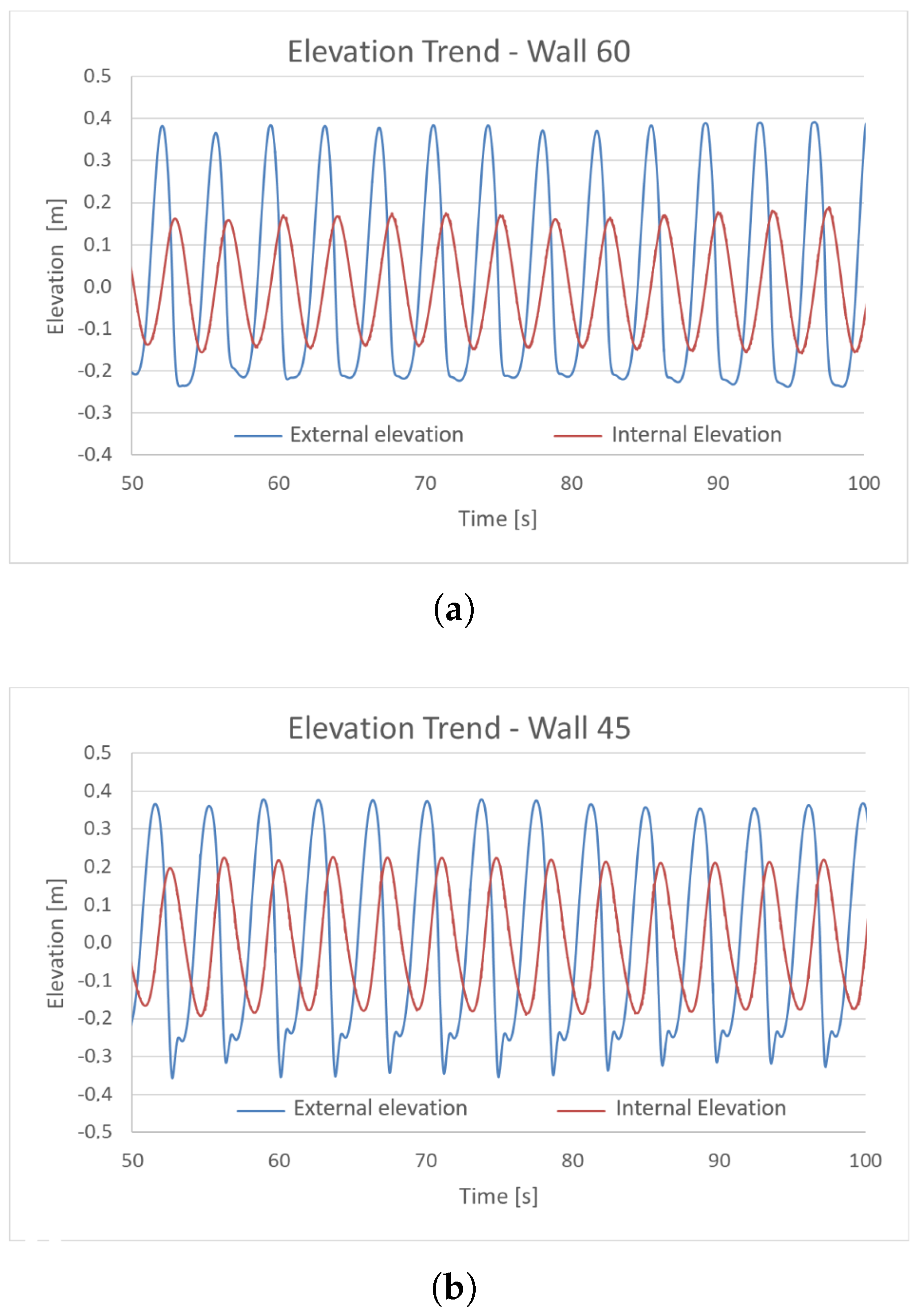
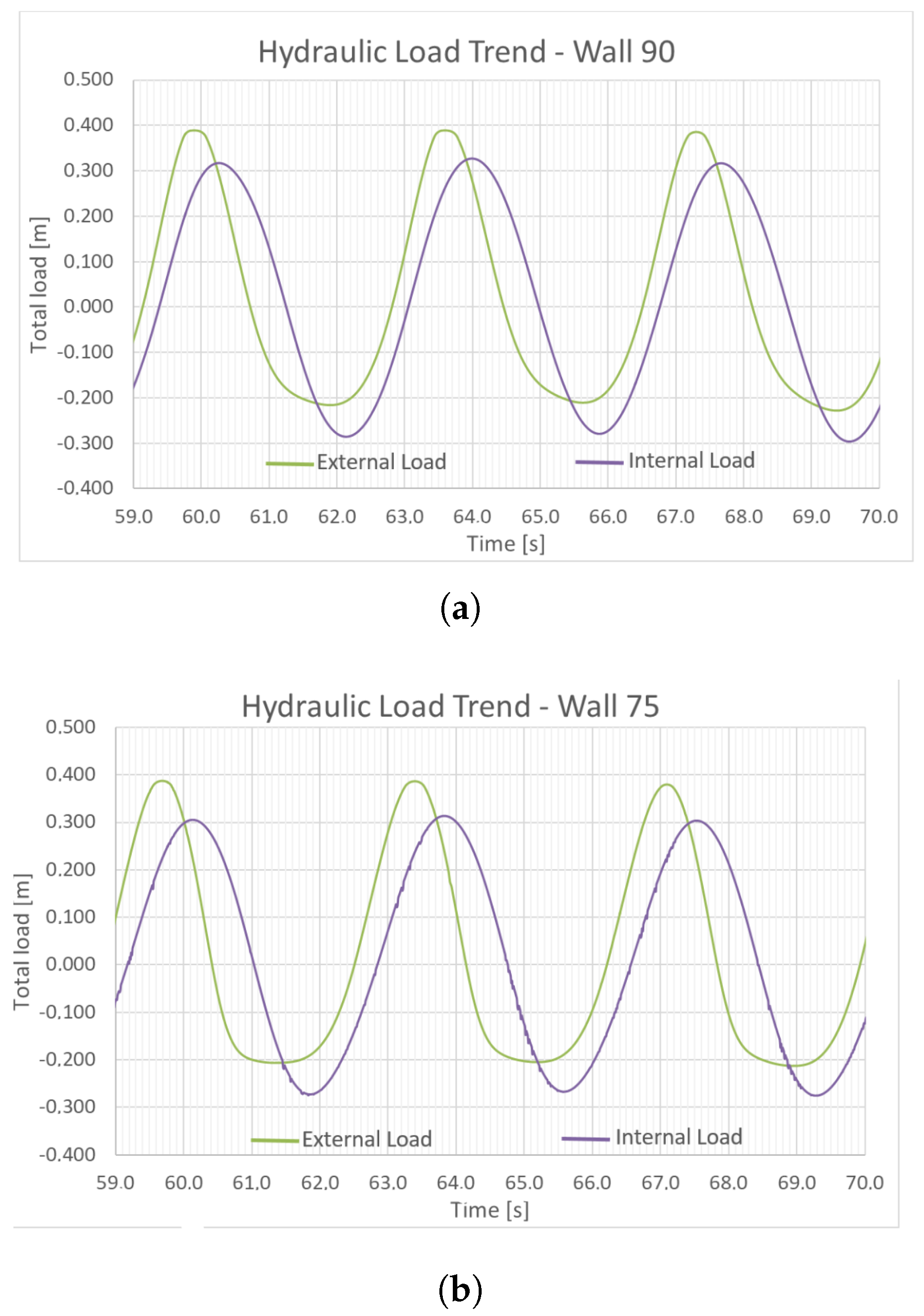
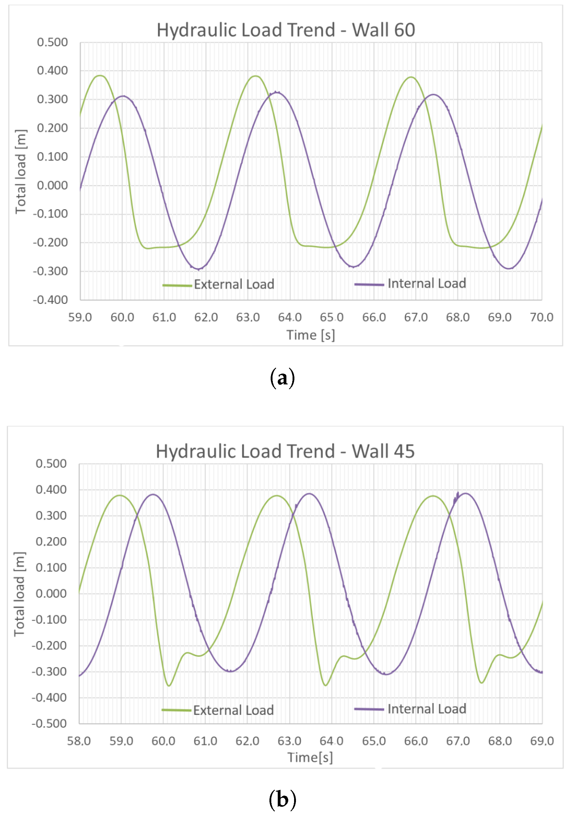
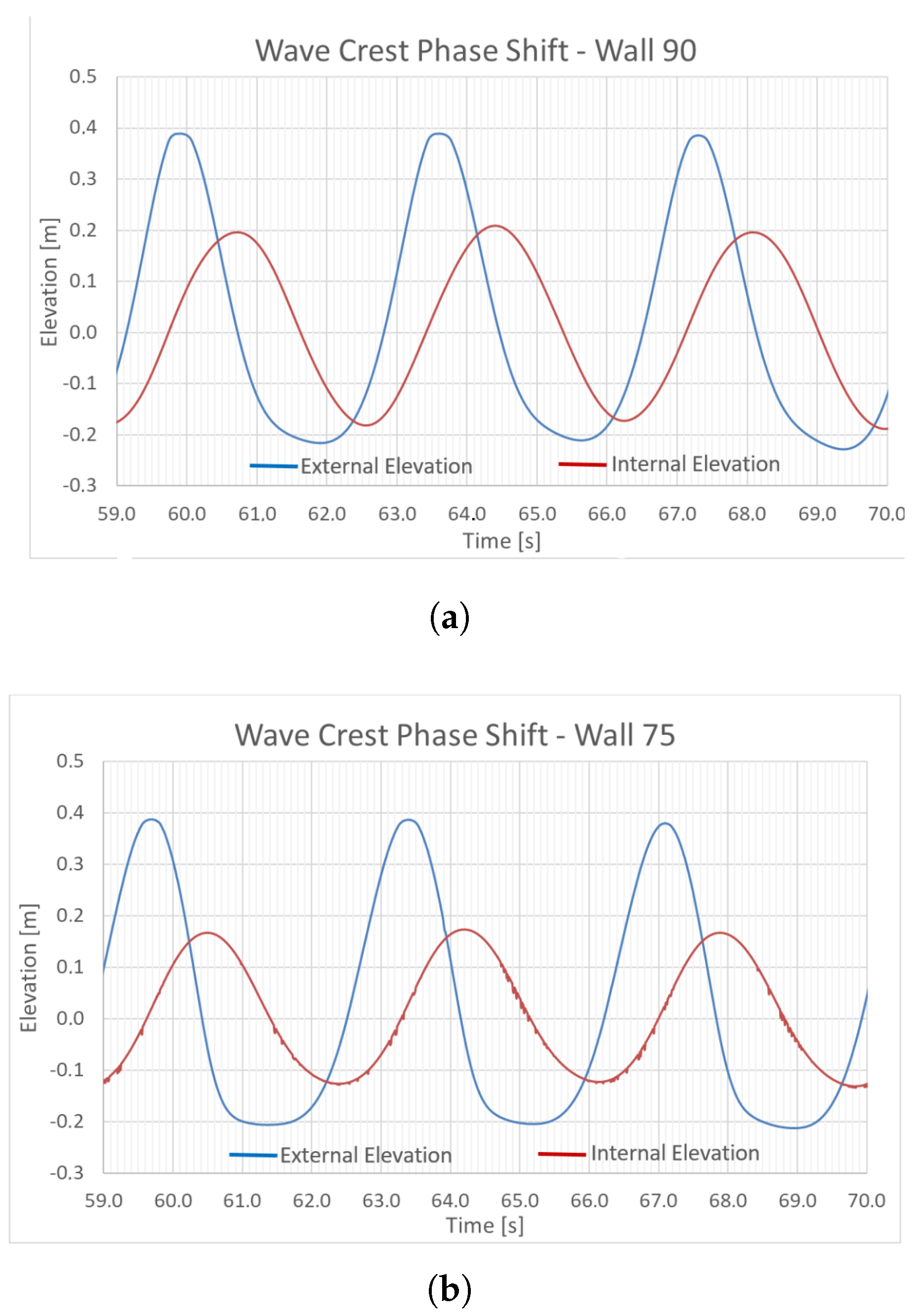
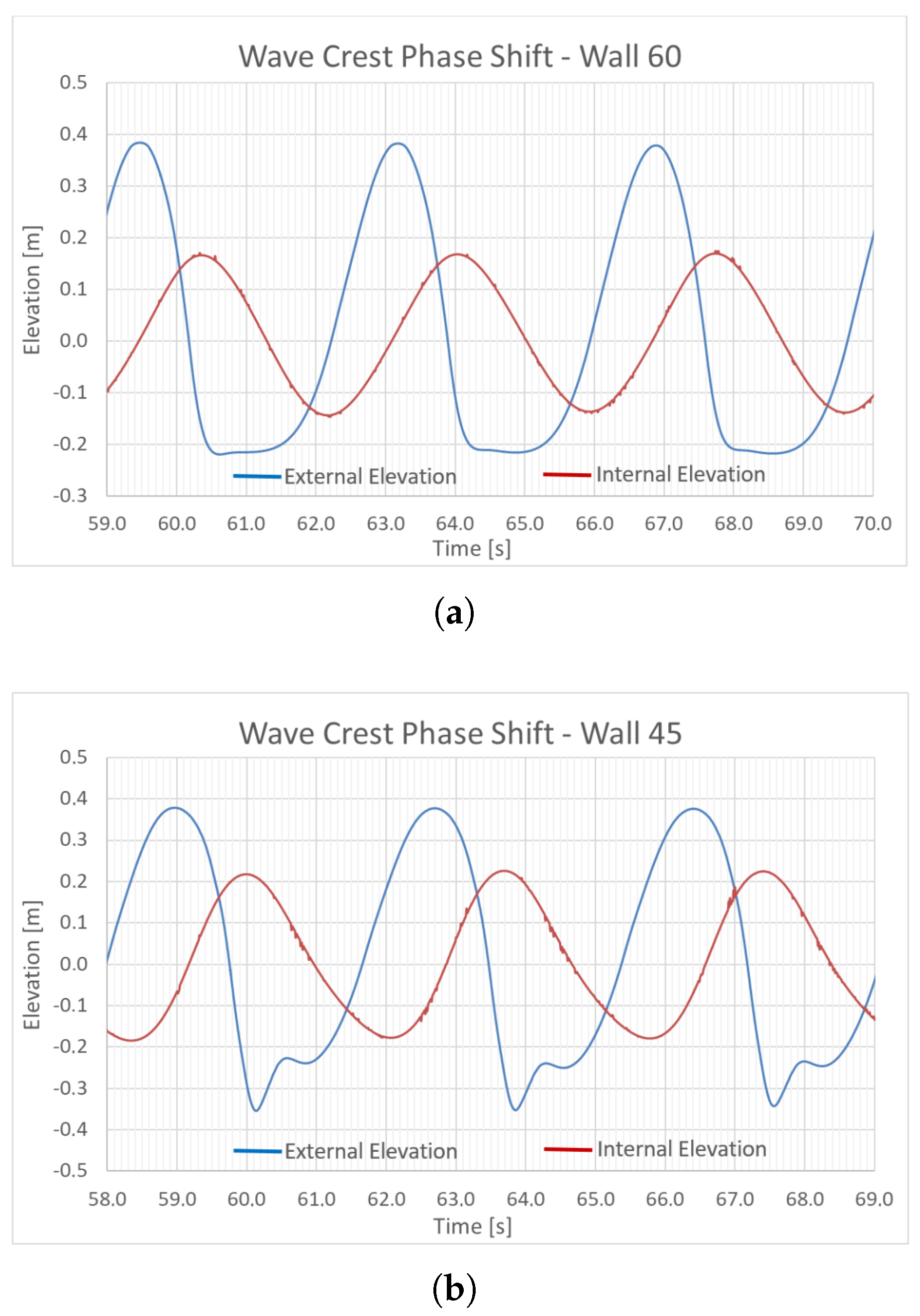
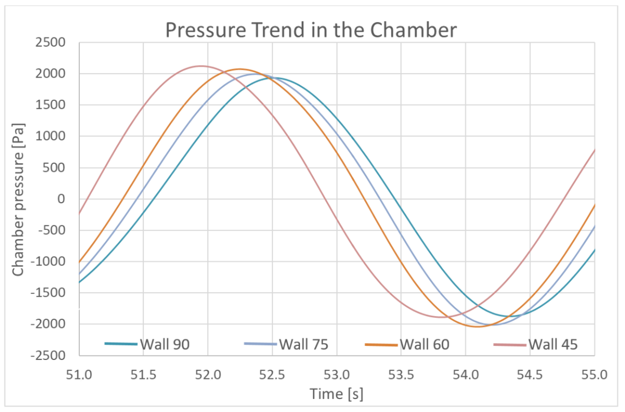
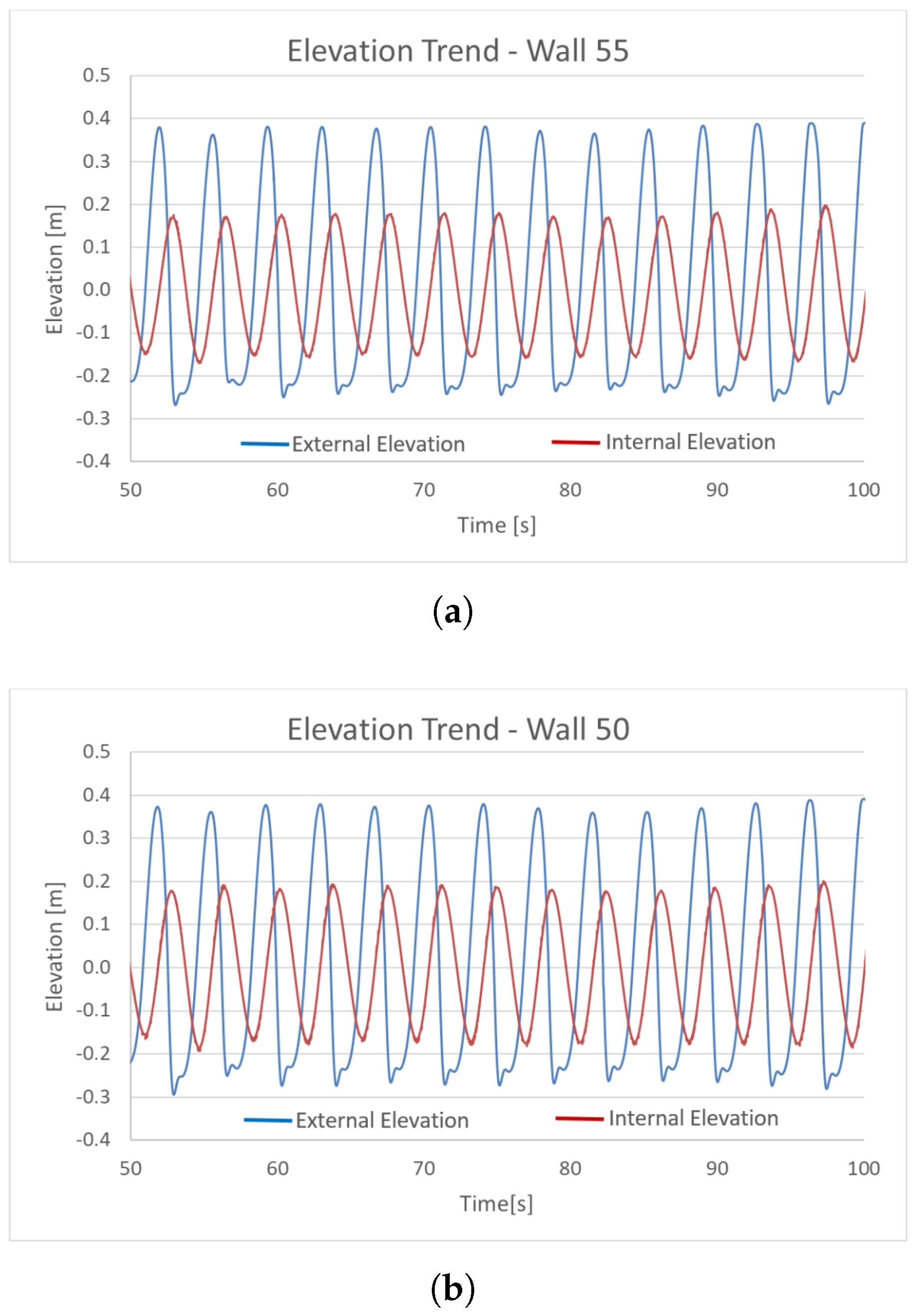
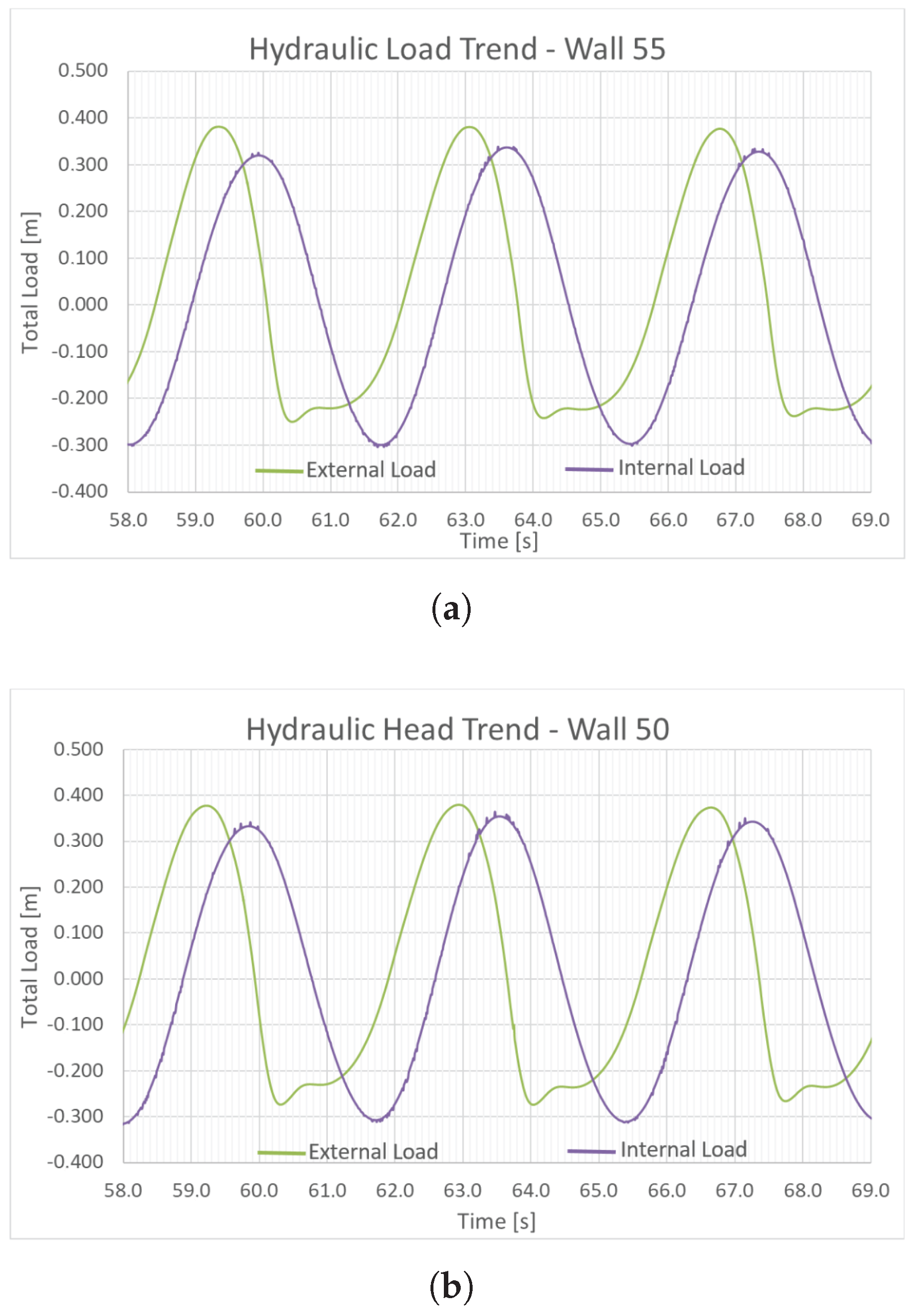
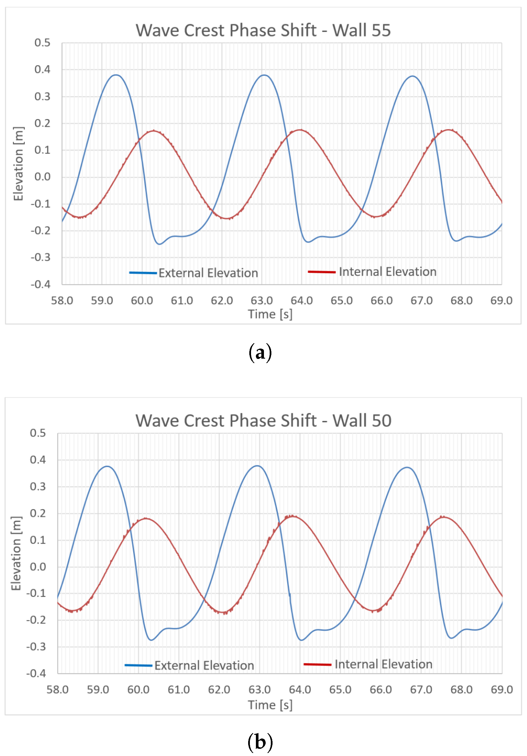
The Final Simulation Results
- (a)
- Elevation trends of the water surface inside and outside the OWC chamber;
- (b)
- Trends in internal and external hydraulic loads;
- (c)
- Phase shift of the wave crest between the internal and external domains;
- (d)
- Pressure profiles and the performance of the PTO system.
5. Conclusions
Author Contributions
Funding
Data Availability Statement
Acknowledgments
Conflicts of Interest
References
- Ross, D. Power from the Waves; Oxford University Press: Oxford, UK, 1995. [Google Scholar]
- Salter, S.H. Wave power. Nature 1974, 249, 720–724. [Google Scholar] [CrossRef]
- Gunn, K.; Stock-Williams, C. Quantifying the global wave power resource. Renew. Energy 2012, 44, 296–304. [Google Scholar] [CrossRef]
- Thorpe, T.W. A Brief Review of Wave Energy; Technical Report R120; Energy Technology Support Unit (ETSU): Harwell, UK, 1999. [Google Scholar]
- Clément, A.; McCullen, P.; Falcão, A.; Fiorentino, A.; Gardner, F.; Hammarlund, K.; Lemonis, G.; Lewis, T.; Nielsen, K.; Petroncini, S.; et al. Wave energy in Europe: Current status and perspectives. Renew. Sustain. Energy Rev. 2002, 6, 405–431. [Google Scholar] [CrossRef]
- Tucker, M.J.; Pitt, E.G. Waves in Ocean Engineering; Elsevier: Oxford, UK, 2001. [Google Scholar]
- Pelc, R.; Fujita, R.M. Renewable energy from the ocean. Mar. Policy 2002, 26, 471–479. [Google Scholar] [CrossRef]
- Korde, U.A. Control system applications in wave energy conversion. In Proceedings of the OCEANS 2000 MTS/IEEE Conference and Exhibition, Conference Proceedings, Providence, RI, USA, 11–14 September 2000; Volume 3, pp. 1817–1824. [Google Scholar] [CrossRef]
- Duckers, L. Wave energy. In Renewable Energy: Power for a Sustainable Future, 2nd ed.; Boyle, G., Ed.; Oxford University Press: Oxford, UK, 2004. [Google Scholar]
- Ahamed, R.; McKee, K.; Howard, I. Advancements of wave energy converters based on power take off (PTO) systems: A review. Ocean Eng. 2020, 204, 107248. [Google Scholar] [CrossRef]
- Baker, N.J.; Mueller, M.A. Direct drive wave energy converters. Rev. Energies Renouvelables 2001, 4, 1–7. [Google Scholar]
- Blanco, M.; Torres, J.; Santos-Herrán, M.; García-Tabarés, L.; Navarro, G.; Nájera, J.; Ramírez, D.; Lafoz, M. Recent Advances in Direct-Drive Power Take-Off (DDPTO) Systems for Wave Energy Converters Based on Switched Reluctance Machines (SRM). In Ocean Wave Energy Systems: Hydrodynamics, Power Takeoff and Control Systems; Samad, A., Sannasiraj, S., Sundar, V., Halder, P., Eds.; Springer International Publishing: Cham, Switzerland, 2022; pp. 487–532. [Google Scholar] [CrossRef]
- Drew, B.; Plummer, A.R.; Sahinkaya, M.N. A review of wave energy converter technology. Proc. Inst. Mech. Eng. Part A J. Power Energy 2009, 223, 887–902. [Google Scholar] [CrossRef]
- Garcia-Teruel, A.; Forehand, D.I.M. A review of geometry optimisation of wave energy converters. Renew. Sustain. Energy Rev. 2021, 139, 110593. [Google Scholar] [CrossRef]
- Berrouche, Y.; Pillay, P. Determination of salinity gradient power potential in Québec, Canada. J. Renew. Sustain. Energy 2012, 4, 053113. [Google Scholar] [CrossRef]
- Cipollina, A.; Micale, G. (Eds.) Sustainable Energy from Salinity Gradients, 1st ed.; Woodhead Publishing Series in Energy; Woodhead Publishing: Sawston, UK, 2016. [Google Scholar]
- Abbas, S.M.; Alhassany, H.D.S.; Vera, D.; Jurado, F. Review of enhancement for ocean thermal energy conversion system. J. Ocean. Eng. Sci. 2022; in press. [Google Scholar] [CrossRef]
- Sakthivel, C.; Pradeep, R.; Rajaskaran, R.; Bharath, S.; Manikandan, S. A review of Ocean Thermal Energy Conversion. In Proceedings of the Conference on Emerging Trends in Electrical, Electronics and Computer Engineering (ETEEC2018), Coimbatore, India, 4 April 2018; pp. 275–280. [Google Scholar]
- Mishra, S.K.; Mohanta, D.K.; Appasani, B.; Kabalcı, E. OWC-Based Ocean Wave Energy Plants; Springer: Singapore, 2021. [Google Scholar]
- Garrido, A.J.; Otaola, E.; Garrido, I.; Lekube, J.; Maseda, F.J.; Liria, P.; Mader, J. Mathematical modeling of oscillating water columns wave-structure interaction in ocean energy plants. Math. Probl. Eng. 2015, 2015, 727982. [Google Scholar] [CrossRef]
- Liu, Z.; Hyun, B.S.; Hong, K.y. Application of Numerical Wave Tank to OWC Air Chamber for Wave Energy Conversion. In Proceedings of the Eighteenth (2008) International Offshore and Polar Engineering Conference, Vancouver, BC, Canada, 6–11 July 2008; The International Society of Offshore and Polar Engineers (ISOPE): Mountain View, CA, USA, 2008; pp. 350–356. [Google Scholar]
- Liu, Z.; Hyun, B.S.; Jin, J.Y. Numerical Analysis of Wave Field in OWC Chamber Using VOF Model. J. Ocean Eng. Technol. 2008, 22, 1–6. [Google Scholar]
- Ren, X.; Ma, Y. Numerical simulations for nonlinear waves interaction with mutiple perforated quasi-ellipse caissons. Math. Probl. Eng. 2015, 2015, 895673. [Google Scholar] [CrossRef]
- Heath, T.V. A review of oscillating water columns. Philos. Trans. R. Soc. A 2022, 370, 235–245. [Google Scholar] [CrossRef]
- Khaleghi, S.; Lie, T.T.; Baguley, C. An Overview of the Oscillating Water Column (OWC) Technologies: Issues and Challenges. J. Basic Appl. Sci. 2022, 18, 98–118. [Google Scholar] [CrossRef]
- Moretti, G.; Malara, G.; Scialò, A.; Daniele, L.; Romolo, A.; Vertechy, R.; Fontana, M.; Arena, F. Modelling and field testing of a breakwater-integrated U-OWC wave energy converter with dielectric elastomer generator. Renew. Energy 2020, 146, 628–642. [Google Scholar] [CrossRef]
- Thiruvenkatasamy, K.; Neelamani, S. On the efficiency of wave energy caissons in array. Appl. Ocean Res. 1997, 19, 61–72. [Google Scholar] [CrossRef]
- Caldarola, F.; Carini, M.; Maiolo, M.; Papaleo, M.A. Iterative mathematical models based on curves and applications to coastal profiles. Mediterr. J. Math. 2024, 21, 178. [Google Scholar] [CrossRef]
- Mandelbrot, B. How Long Is the Coast of Britain? Statistical Self-Similarity and Fractional Dimension. Science 1967, 156, 636–638. [Google Scholar] [CrossRef]
- Antoniotti, L.; Caldarola, F.; Maiolo, M. Infinite numerical computing applied to Peano’s, Hilbert’s, and Moore’s curves. Mediterr. J. Math. 2020, 17, 99. [Google Scholar] [CrossRef]
- Caldarola, F. The exact measures of the Sierpiński d-dimensional tetrahedron in connection with a Diophantine nonlinear system. Commun. Nonlinear Sci. Numer. Simul. 2018, 63, 228–238. [Google Scholar] [CrossRef]
- Caldarola, F. The Sierpiński curve viewed by numerical computations with infinities and infinitesimals. Appl. Math. Comput. 2018, 318, 321–328. [Google Scholar] [CrossRef]
- Caldarola, F.; Maiolo, M. On the Topological Convergence of Multi-rule Sequences of Sets and Fractal Patterns. Soft Comput. 2020, 24, 17737–17749. [Google Scholar] [CrossRef]
- Holmes, M.H. Introduction to Perturbation Methods; Springer: New York, NY, USA, 2013. [Google Scholar]
- Dean, R.G.; Dalrymple, R.A. Water Wave Mechanics for Engineers and Scientists; World Scientific: Singapore, 1991. [Google Scholar]
- McCormick, M.E. Ocean Engineering Mechanics; Cambridge University Press: Cambridge, UK, 2010. [Google Scholar]
- Versteeg, H.K.; Malalasekera, W. An Introduction to Computational Fluid Dynamics: The Finite Volume Method; Pearson Education: London, UK, 2007. [Google Scholar]
- Pope, S. Turbulent Flows; Cambridge University Press: Cambridge, UK, 2000. [Google Scholar]
- Hayati, M.; Nikseresht, A.H.; Taherian Haghighi, A. Sequential optimization of the geometrical parameters of an OWC device based on the specific wave characteristics. Renew. Energy 2020, 161, 386–394. [Google Scholar] [CrossRef]
- Zeghadnia, L.; Robert, J.L.; Achour, B. Explicit solutions for turbulent flow friction factor: A review, assessment and approaches classification. Ain Shams Eng. J. 2019, 10, 243–252. [Google Scholar] [CrossRef]


| Symbol | Reference | Formula | Value |
|---|---|---|---|
| a | Front wall sinking | 0.8 m | |
| b | Chamber width | 1.9 m | |
| c | Visible external height | - | 4 m |
| d | Front wall thickness | 0.5 m | |
| f | Bottom step height | 1.6 m | |
| I | Bottom step length | 9 m | |
| s | Bottom step inclination | - | 90° |
| Frontal Wall | ||||
|---|---|---|---|---|
| ≈10.4% | ≈11.6% | ≈12.5% | ≈11.5% |
| Frontal Wall | ||||
|---|---|---|---|---|
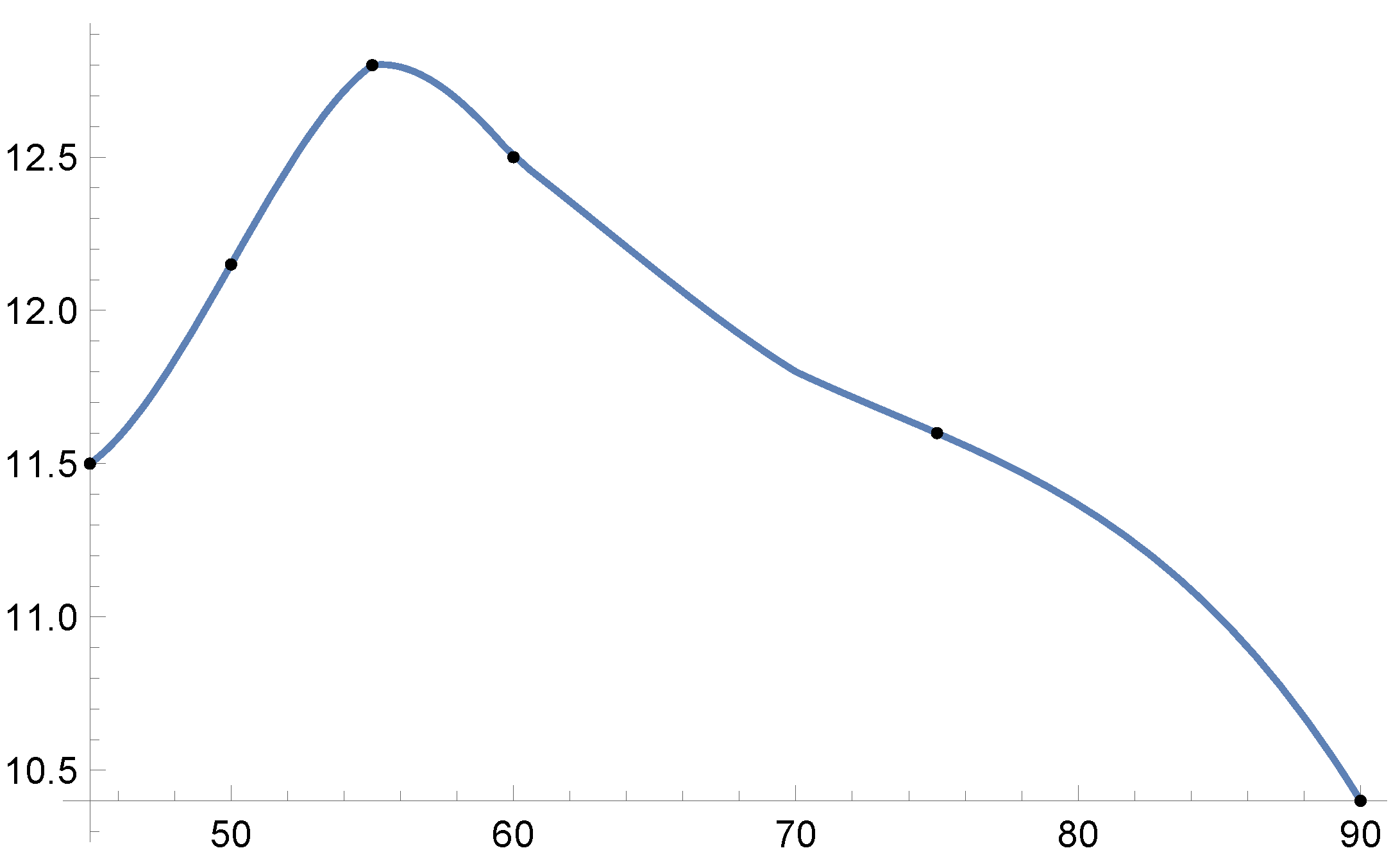
| ≈12.5% | ≈12.8% | ≈12.15% | ≈11.5% |
Disclaimer/Publisher’s Note: The statements, opinions and data contained in all publications are solely those of the individual author(s) and contributor(s) and not of MDPI and/or the editor(s). MDPI and/or the editor(s) disclaim responsibility for any injury to people or property resulting from any ideas, methods, instructions or products referred to in the content. |
© 2025 by the authors. Licensee MDPI, Basel, Switzerland. This article is an open access article distributed under the terms and conditions of the Creative Commons Attribution (CC BY) license (https://creativecommons.org/licenses/by/4.0/).
Share and Cite
Caldarola, F.; Carini, M.; Costarella, A.; De Raffele, G.; Maiolo, M. Physical–Mathematical Modeling and Simulations for a Feasible Oscillating Water Column Plant. Mathematics 2025, 13, 2219. https://doi.org/10.3390/math13142219
Caldarola F, Carini M, Costarella A, De Raffele G, Maiolo M. Physical–Mathematical Modeling and Simulations for a Feasible Oscillating Water Column Plant. Mathematics. 2025; 13(14):2219. https://doi.org/10.3390/math13142219
Chicago/Turabian StyleCaldarola, Fabio, Manuela Carini, Alessandro Costarella, Gioia De Raffele, and Mario Maiolo. 2025. "Physical–Mathematical Modeling and Simulations for a Feasible Oscillating Water Column Plant" Mathematics 13, no. 14: 2219. https://doi.org/10.3390/math13142219
APA StyleCaldarola, F., Carini, M., Costarella, A., De Raffele, G., & Maiolo, M. (2025). Physical–Mathematical Modeling and Simulations for a Feasible Oscillating Water Column Plant. Mathematics, 13(14), 2219. https://doi.org/10.3390/math13142219