Quantales for Fuzzy Sets and Relations of Higher Types

Abstract

In this paper, we open up more possibilities to define higher types of fuzzy sets in a mixed way. In doing so, we show that there are essentially two alternative definitions for fuzzy sets of higher types, one of which is widely adopted in the literature, and one where the unit interval, or subsets thereof, is used to represent membership values. The other alternative definition opens up new perspectives for the use of fuzzy sets of higher types, and it promotes the use of other algebraic structures of sets of membership values, where quantales are seen as particularly useful, also in applications. The paper also underlines the importance of making distinctions between “computing with fuzzy” and “fuzzy computing” and understanding the difference between “logic with fuzzy” and “fuzzy logic”.

1. Introduction

Zadeh [1,2] introduced the notion of fuzzy sets of higher types by saying that ${\mu }_A\left(x\right)$, for a fuzzy set ${\mu }_A$ of type 2, is “allowed to be a fuzzy set of $[0,1]$”.

In Zadeh’s vocabulary and notation, a “fuzzy set of $[0,1]$” is a function $\mu :[0,1]\to [0,1]$, i.e., a fuzzy set of type 2, according to [1,2], is

$$\mu :X\to {[0,1]}^{[0,1]}$$

where ${[0,1]}^{[0,1]}$ is the set of all functions $f:[0,1]\to [0,1]$.

For any $x\in X$, $\mu \left(x\right)$ is then a function

$$\mu \left(x\right):[0,1]\to [0,1]$$

where the range of fuzzy sets of type 2 is in the

$${[0,1]}^{[0,1]}$$

and the set of fuzzy sets of type 2, over X, is

$${\left({[0,1]}^{[0,1]}\right)}^X$$

Generally, $Y^X$ denotes the set of all functions $f:X\to Y$. We use the power notation more frequently, particularly in Section 4.

In their Definition 3.22 in [1], with exactly the same wording as in Definition 3.1 in [2], Zadeh defines a fuzzy set to be of type n, $n=2,3,\dots$, if its membership function ranges over fuzzy sets of type $n-1$, further stating that the membership function of a fuzzy set of type 1 ranges over the interval $[0,1]$.

The range $[0,1]$ of a fuzzy set of type 1 appears both in the base and in the exponent of the type 2 range ${[0,1]}^{[0,1]}$.

For fuzzy sets of type 3, the situation opens up two alternatives for the range, as the range may be

$${[0,1]}^{\left({[0,1]}^{[0,1]}\right)}$$

or, alternatively,

$${\left({[0,1]}^{[0,1]}\right)}^{[0,1]}$$

Similarly, for fuzzy sets of type 4, the range is

$${[0,1]}^{\left({[0,1]}^{\left({[0,1]}^{[0,1]}\right)}\right)}$$

(1)

or, alternatively,

$${\left({\left({[0,1]}^{[0,1]}\right)}^{[0,1]}\right)}^{[0,1]}$$

(2)

and so on for fuzzy sets of type n.

This indeed leads to two different definitions for fuzzy sets of higher types, and in Section 4, we show how the alternative definitions can be provided recursively.

Before formulating the recursive definitions of fuzzy sets of type n, in Section 2, we provide a brief historical overview of fuzzy sets and fuzzifications, including discussions on traditions related to notations. In Section 3, we discuss algebraic structures equipped with the set of membership values, and we discuss the advantages of using quantales as possessing a suitable algebraic structure.

In Section 5, we introduce the Design Structure Matrix (DSM) as an application area, where fuzzy sets of higher types in fact already are used but not recognized in application development by academia and industry. Whereas in Section 4 we extend the range of fuzzy sets to embrace more elaborate structure, in Section 6, we discuss the domain X and how it can be extended with structure affecting topics and features in fuzzy logic.

Section 7 concludes the paper.

2. Fuzzy Sets and Fuzzifications

In [3], Zadeh introduced the notion of fuzzy sets using the notation $f_A$ for a “fuzzy set A in X” and defining it as the function $f_A:X\to [0,1]$. Zadeh came later to use the notation ${\mu }_A$ instead of $f_A$, and the ${\mu }_A$ notation has been widely used in the literature.

Zadeh remarks in their second footnote in [3] that the domain of the function may be restricted to a subset of X, without explicitly saying that such a restriction will define a partial function. In their third footnote, Zadeh remarks that the unit interval $[0,1]$ may be replaced by “a suitable partially ordered set”. Zadeh’s introductory text speaks about “a continuum of grades of membership”, so it is not clear what kind of partially ordered structures Zadeh had in mind at the time of writing their 1965 paper. Zadeh may have had lattices in mind as “suitable” partially ordered sets, as a lattice structure has meet and join operations similar to $min$ and $max$ for the unit interval, where $min$ and $max$ provide the unit interval with a partial order and with the structure of a lattice.

Some years later, communicating with Zadeh, Goguen [4] introduced L-fuzzy sets, where the set L of membership values is discussed in light of a wide range of structures, including complete distributive lattices, frequently used in the fuzzy literature.

Zadeh’s notation ${\mu }_A:X\to [0,1]$ for fuzzy sets (of type 1) may lead to some confusion. The characteristic function ${\chi }_A:X\to \{0,1\}$ of a subset $A\subseteq X$ is

$${\chi }_A\left(x\right)=\left\{\begin{array}{cc}1,\hfill & \mathrm{if}x\in A\hfill \\ 0,\hfill & \mathrm{if}x\notin A\hfill \end{array}\right.$$

where the function is indexed by A, the set for which the function “is characteristic”. The index A is the set for which ${\chi }_A$ is its characteristic function. However, in the case of ${\mu }_A$, A is not a set, and it is actually nothing in itself but rather just an indexing symbol in the notation for the membership function so that we may informally say “A is a fuzzy subset”. The index A could in fact be dropped so that a fuzzy $\mu$ on a set X can be defined as a function $\mu :X\to [0,1]$. Alternatively, A could be the actual notation for the fuzzy set, so that the fuzzy set is denoted by $A:X\to [0,1]$, making “$\mu$” obsolete in the notation. The notation “A” for a fuzzy set was adopted by Goguen in [4], where A is an L-fuzzy set over X whenever A is the function $A:X\to L$.

Notations connected with fuzzy sets may indeed be confusingly intertwined, if the notions of “set” and “function” are not clearly separated in the notation. If we say that the function $\mu :X\to [0,1]$ is a “fuzzy set over X”, we may introduce the set

$$A_{\mu }=\{(x,\mu \left(x\right))\mid x\in X\}$$

(3)

which is a subset of the product set $X\times [0,1]$, so that the $A_{\mu }$ as a set defined by (3) “represents” the fuzzy set $\mu$ as function. In this case, $\mu$ is given and it enables us to define $A_{\mu }$.

We may also have it the other way around, i.e., we have subset $A\subseteq X\times [0,1]$ which, in order to enable us to define a fuzzy set, must fulfill the conditions

(a)

For each $x\in X$ there exists an $\alpha \in [0,1]$ such that $(x,\alpha )\in A$;

(b)

If $(x,{\alpha }_1),(x,{\alpha }_2)\in A$, then ${\alpha }_1={\alpha }_2$.

If $A\subseteq X\times [0,1]$ fulfills conditions (a) and (b), we may define a fuzzy set $\mu :X\to [0,1]$ according to $\mu \left(x\right)=\alpha$ whenever $(x,\alpha )\in A$. In this case we obtain $A_{\mu }$ to appear as in (3).

Now we clearly see how A, or $A_{\mu }$, is a set whereas $\mu$, or ${\mu }_A$, is a function. Confusion may indeed arise if we use “A” interchangeably for both the function and the set representing the function.

These notational remarks may seem superfluous, but when we provide our notations for fuzzy sets of higher types we have to treat indices carefully so as to not introduce ambiguous notation because of the intuitive meanings of symbols that are not defined in the context.

Zadeh’s summation and integral notations, introduced in [1], are informal notations, and may invite additional intuitive understandings of fuzzy sets. Misuse of these notations could easily spill over to include non-intended hidden properties in the formal treatment of fuzzy sets.

In [1] Zadeh writes that a finite set

$$U=\{u_1,\dots ,u_n\}$$

can be expressed as

$$U=u_1+\cdots +u_n$$

or

$$U=\sum _{i=1}^n{u}_i$$

where a theoretically precise set notation would, respectively, be

$$U=\left\{u_1\right\}\cup \cdots \cup \left\{u_n\right\}$$

and

$$U=\bigcup _{i=1}^n\left\{u_i\right\}$$

Zadeh also introduced a similar “summation” notation for a fuzzy set over U according to

$$A={\mu }_1/u_1+\cdots +{\mu }_n/u_n$$

or

$$A=\sum _{i=1}^n{\mu }_i/u_i$$

where ${\mu }_i$, $i=1,\dots ,n$, are “membership grades” attached to elements $u_i\in U$. The theoretically precise set notations would, respectively, be

$$A=\left\{(u_1,{\mu }_1)\right\}\cup \cdots \cup \left\{(u_n,{\mu }_n)\right\}$$

and

$$A=\bigcup _{i=1}^n\left\{(u_i,{\mu }_i)\right\}$$

For infinite sets U, and given a fuzzy set ${\mu }_A:U\to [0,1]$, Zadeh introduced the “integral” notation

$$A={\int }_U{\mu }_A\left(u\right)/u$$

which in theoretically precise set notation would be

$$A=\bigcup _{u\in U}\left\{(u,{\mu }_A\left(u\right))\right\}$$

In this paper, we prefer to avoid using Zadeh’s summation and integral notations so as to not invite intuitive and informal interpretations of sets and functions representing fuzzy sets.

Note also how notation is informal in expressions for fuzzy set operations, e.g., in the case of the “union” of two fuzzy sets ${\mu }_A$ and ${\mu }_B$, with sets A and B defined as in (3). Fuzzy set “union” is defined as

$${\mu }_{A\cup B}\left(x\right)=max({\mu }_A\left(x\right),{\mu }_B\left(x\right))$$

(4)

but the symbol ‘∪’ in (4) is not the symbol for a union of sets, i.e., ‘$A\cup B$’ is not the set union of A and B as defined by (3).

In [3], Zadeh defines constructions for functions that provide mappings and inverse mappings of fuzzy sets. More precisely, as $f:X\to Y$ and using the notation for L-fuzzy sets, if $\beta :Y\to L$ is an L-fuzzy set on Y, then f defines an L-fuzzy $\alpha :X\to L$ on X by

$$\alpha \left(x\right)=\beta \left(f\right(x\left)\right)$$

Conversely, if an L-fuzzy set $\alpha :X\to L$ is known, then f defines an L- fuzzy set $\beta :Y\to L$ by

$$\beta \left(y\right)=\left\{\begin{array}{cc}\underset{y=f\left(x\right),x\in X}{\bigvee }\alpha \left(x\right),\hfill & \mathrm{if}\mathrm{there}\mathrm{exists}x\in X\mathrm{such}\mathrm{that}y=f\left(x\right)\hfill \\ 0,\hfill & \mathrm{otherwise}\hfill \end{array}\right.$$

(5)

which is Zadeh’s Extension Principle, which was already defined in [3] but was not called the Extension Principle until the publication of [1].

In case both $\alpha$ and $\beta$ are given, the way f is “structure preserving” between these fuzzy sets was explored in [5], where, using category theoretical language, f is said to be a morphism whenever

$$\alpha \left(x\right)\le \beta \left(f\right(x\left)\right)$$

(6)

Clearly, if f defines $\beta$ as in (5), then f becomes a morphism, but there are indeed other morphisms between $\alpha$ and $\beta$. In other words, definition (5) viewed as a morphism condition is stronger than the morphism condition (6) proposed in [5]. Goguen was in [5] then able to extend the category $\mathtt{Set}$ of ordinary sets as objects and ordinary functions as morphisms to the category $\mathtt{Set}\left(L\right)$ where objects are L-fuzzy sets over X, $\mu :X\to L$, and morphisms are functions $f:X\to Y$ that fulfill the morphism condition (6).

On fuzzification, and often based on the Extension Principle, there are various options for extending properties and expression using sets to enable the involvement of fuzzy sets. Fuzzy topology, as introduced in [6], was defined simply by using fuzzy set operations in place of set operations. A fuzzy magma, as introduced in [7], with magmas (see Section 3) as a group $(G,\ast )$ over a fuzzy set $\mu :G\to L$, is defined as fulfilling $\mu (a\ast b)\ge \mu \left(a\right)\wedge \mu \left(b\right)$, for all $a,b\in G$. Inspired by such fuzzifications in topology and algebra, similar and often rather straightforward fuzzifications were developed in other branches of mathematics, which certainly was one of the main reasons for the accelerated growth of interest in fuzzy systems, in particular during the 1970s and 1980s. At the same time, AI with neural networks became popular and widespread, leading to interaction between the fuzzy and neural network communities. The IEEE conferences for Fuzzy Systems and Neural Networks were co-located in Spring 1993 in San Francisco, where the printed proceedings, in several volumes, contained neural network-based papers more than twice as much as the fuzzy systems papers, while also including many “neural fuzzy” approaches, in particular within engineering applications as involving fuzzy controllers extended with learning capabilities.

3. Lattices, Semigroups, and Quantales

The unit interval $[0,1]$ as a continuum has been and still is the dominating range of fuzzy sets, particularly in applications involving decision support using rule-based systems. Finite sets with structure had long been used before the publication of [3], in particular in many-valued logic, to extend the notion of “two-valued truth”. Three-valued logic was widely used in logic and in work related to the foundations of mathematics during early decades of the 20th century. A survey of these efforts can be found in [8].

Extending two-valued truth in logic to three-valued truth still does not invite using other types of logical operators than those used in two-valued logic. Whereas in two-valued logic the boolean operators are unique, in three-valued logic, there are several ways to define conjunction and disjunction, all leading to three-valued logics with their own distinctive properties. The underlying order of truth values in three-valued logic is also still just a chain, and the middle value was always treated as something that is neither true nor false.

We may also recall how the Sheffer stroke can be used to define all other logical operators when working with two-valued truth, but for many-valued logic in general there are no similar representabilities as the number of options for operators grows exponentially.

Going beyond three values for truth, even to using as little as five and six values for truth and membership, opens up a surprisingly wide spectrum of opportunities for investigating the algebraic structure of the set of truth values. The underlying order structure may no longer be a chain, and, more importantly, working only with conjunction and disjunction as binary operators becomes a restriction, which calls for adding other semigroup operators that possess order-preserving-like properties.

Adding a semigroup operation and requiring it to be distributive with operations providing order relations in the algebra of truth and membership values will essentially introduce a “new multiplication” distinct from the conjunction operator. The distributivity of such an added multiplication operator is suitably assumed to be distributive with respect to disjunction, similar to the situation in distributive lattices concerning conjunction and disjunction.

We therefore advocate for the use of quantales [9] as the underlying algebraic structure for membership in fuzzy sets, so whenever we speak of “Q-fuzzy” in the sense of [4], we assume that Q is a quantale.

In this section, we now discuss certain order-theoretic and algebraic structures needed to construct the order and algebra of fuzzy sets. In particular we present quantales with properties that are useful in many-valued logic, and we also show how even smaller number of membership values in a quantale lead to a wide range of opportunities in applications.

To begin with, recall that one of the main ideas of fuzzy sets is to put elements of a set X in order (by using ’grades’) and combine these orders to receive a final order. We start by providing some viewpoints about lattices. For more details on lattices, see, for example, [10].

A partially ordered set X, denoted by $(X,\le )$, is a lattice if every two-element set $\{x_1,x_2\}\subseteq X$ has an infimum and supremum, i.e., greatest lower bound and lowest upper bound in X, denoted by $x_1\wedge x_2$ and $x_1\vee x_2$, respectively. The operations ∧ and ∨ are called meet and join, respectively, logically corresponding to conjunction and disjunction. A lattice $(X,\le ,\wedge ,\vee )$ may be written case-dependently by X, $(X,\le )$, or $(X,\wedge ,\vee )$.

Given a lattice $(X,\wedge ,\vee )$, the corresponding partial order ≤ satisfies $x_1\le x_2$ if and only if $x_1=(x_1\wedge x_2)$, or, if and only if $x_2=(x_1\vee x_2)$. These two criteria are equivalent because of the absorption laws. Additionally, ∧ and ∨ are idempotent, commutative, and associative operations. Note that one may first have an algebra $(X,\wedge ,\vee )$ and then generate a partial order ≤ (if it exists) to have a lattice, or alternatively, first have a partially ordered set $(X,\le )$ and then generate operations ∧ and ∨ (if they exist) to have a lattice.

A lattice $(X,\le )$ is complete whenever every $A\subseteq X$ has an infimum and supremum in X, denoted by $\bigwedge A$ and $\bigvee A$, respectively. It is evident that in this case, X contains the smallest element, ⊥ (universal lower bound), as well as the largest element, ⊤ (universal upper bound), given the lattice partial order. Focusing on lattice operations with universal lower and upper bounds, one may denote the lattice as $(X,\wedge ,\vee ,\perp ,\top )$.

Lattices may be equipped with additional properties, with distributivity being one such typical additional axiom. A lattice is said to be distributive if

$$\begin{array}{cc}\hfill x_1\vee (x_2\wedge x_3)& =(x_1\vee x_2)\wedge (x_1\vee x_3)\hfill \\ \hfill x_1\wedge (x_2\vee x_3)& =(x_1\wedge x_2)\vee (x_1\wedge x_3)\hfill \end{array}$$

for all $x_1,x_2,x_3\in X$.

Finite lattices are always complete, but they are not always distributive. Finite lattices that are chains, i.e., the partial ordering is the total, are always distributive.

Let us at this point remind ourselves that the names of the elements in X are just symbols, i.e., we should never assume a property not mentioned to be valid simply because a symbol looks like a symbol often used in another mathematical context where the symbol is connected with other properties.

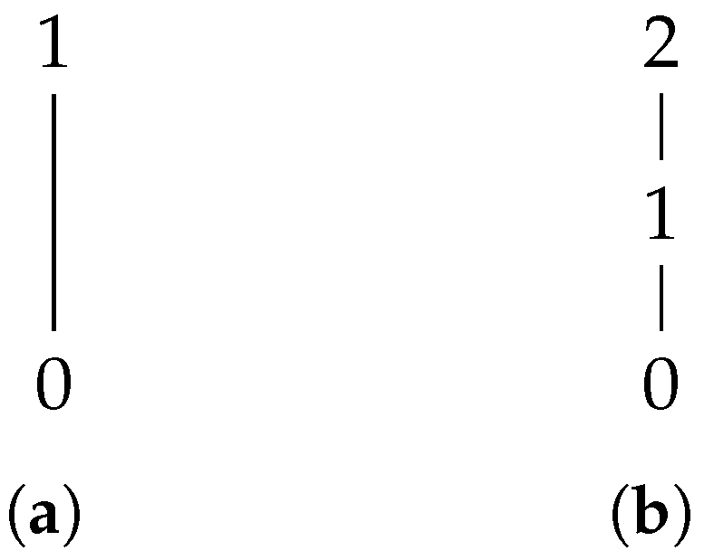
If X is 2-pointed, i.e., $X=\{\perp ,\top \}$, there is only one lattice over X. Similarly, for the 3-point situation $X=\{\perp ,e,\top \}$, there is only one lattice. The elements in X may indeed be named or symbolized in different ways, and in graphical presentations of lattices, we sometimes find it suitable to write $X=\{0,1,\dots ,n-1\}$, for the n-point set in a lattice, where 0 is the bottom element, and $n-1$ is the top element.

There is indeed only one lattice, the chain, on 2-point and 3-point sets, as shown in Figure 1.

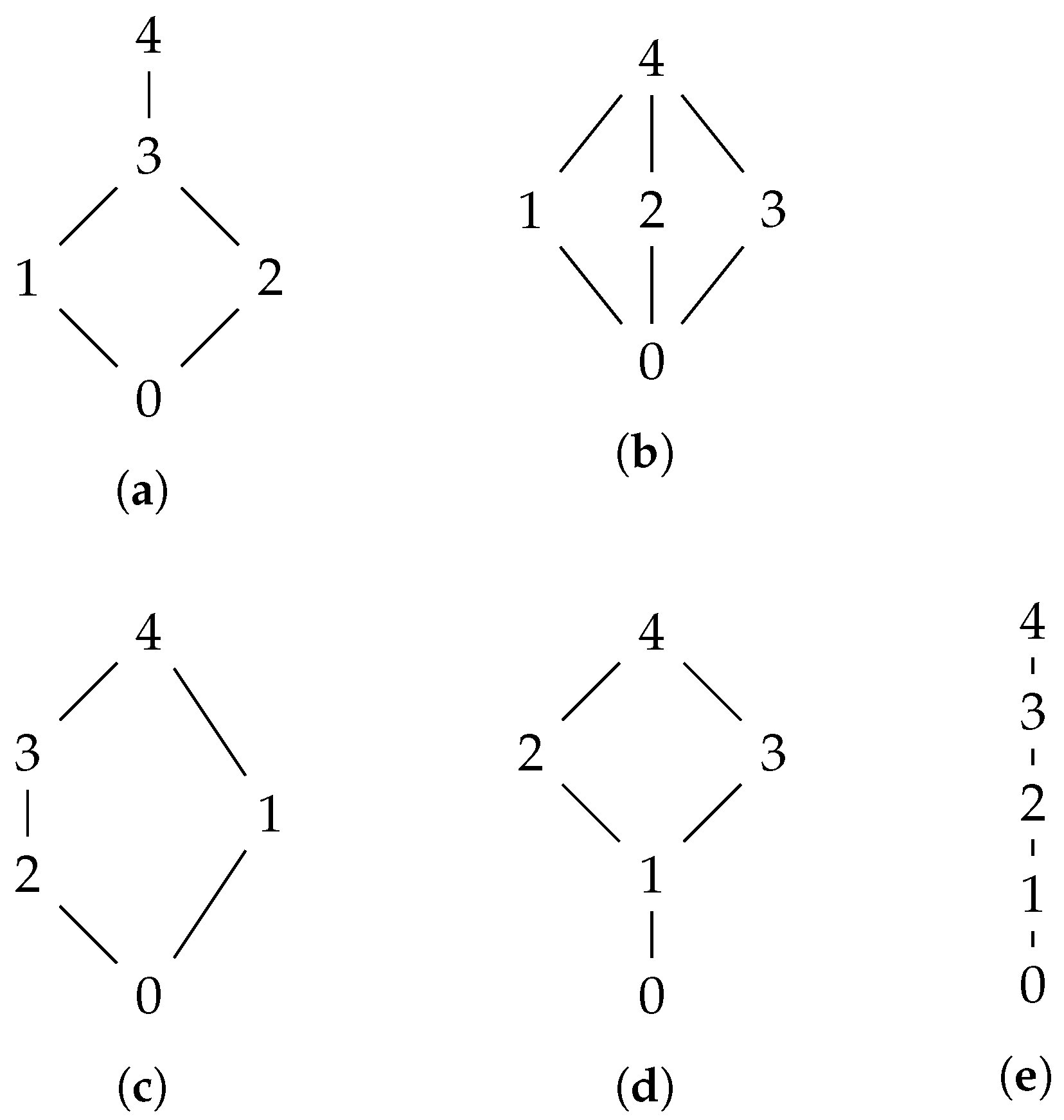
There are two lattices on a 4-point set, as shown in Figure 2.

There are 5 lattices on a 5-point set, shown in Figure 3.

Note that, in the case of the “diamond” lattice with four elements, we may see it as 3-point subchain, e.g., on the set $\{0,1,3\}$ with element ‘2’ as a “sidelined” point with respect to the subchain. This is more apparent in the case of 5-point lattices, where lattices Nr 1, 3, and 4 can be viewed as containing subchains with four elements together with one sidelined element, which is “situated” differently in the respective lattice. The sidelined elements may, particularly in some applications, be understood as a “not known” membership or truth value, and doing so, quantales thus enable us to compute with missing values.

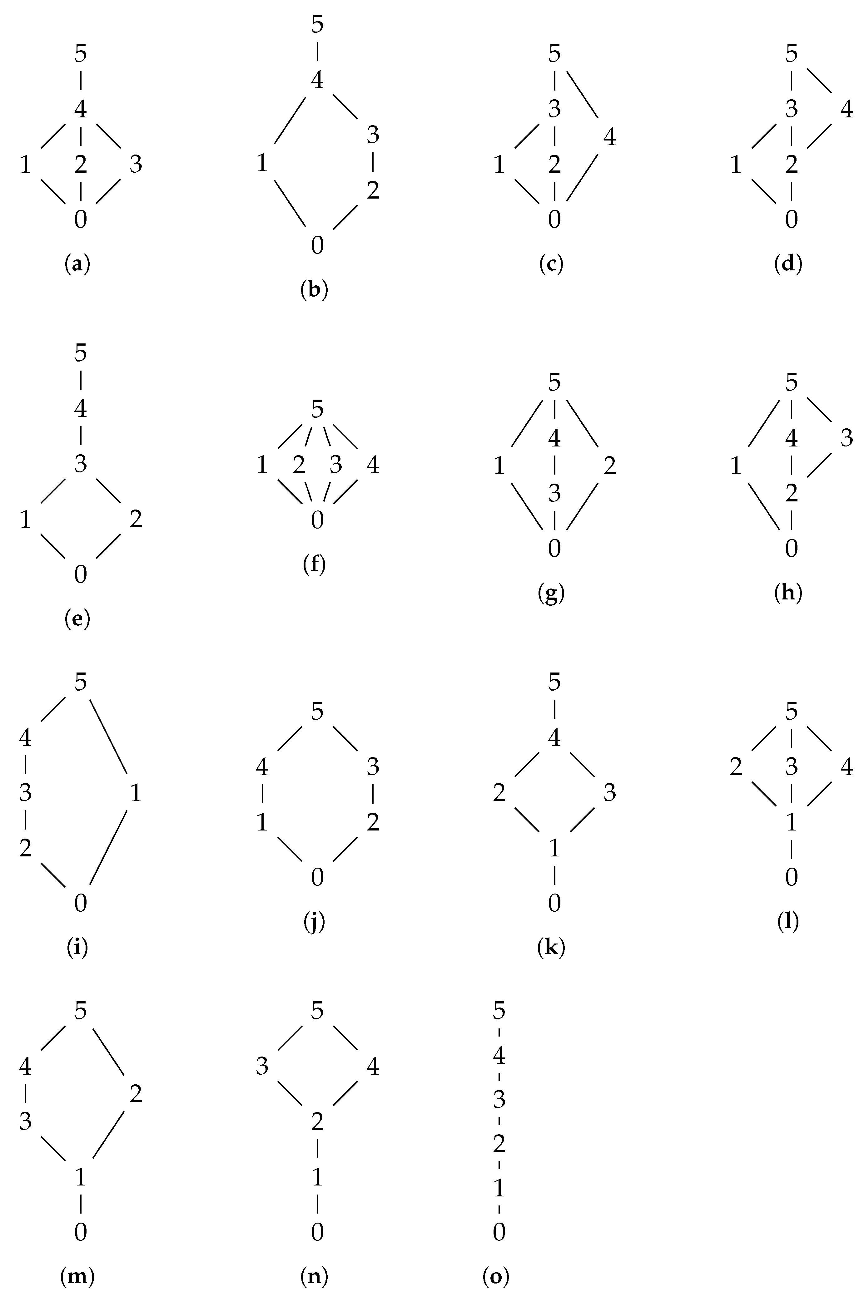
There are 15 lattices on a 6-point set, shown in Figure 4.

Note that for 6-point sets we have six lattices with five chains together with a sidelined element. These are lattices Nr 2, 5, 9, 11, 13, and 14, all with a different “location” for the sidelined element with respect to the subchain. For example, in lattice (i) Nr 9, the sidelined element 1 is below the top and above the bottom element but unordered or unrelated to all other elements. Lattice (k) Nr 11 is similar, but then only elements 2 or 3 are unordered with respect to each other. Lattices (b) Nr 2 and (e) Nr 5 have sideline elements that are in a “more pessimistic way” ordered with respect to the other elements, whereas lattices (m) Nr 13 and (n) Nr 14 are correspondingly “optimistic”.

Elements in the subchain can be renamed as desired and as best-suited for an application, e.g., when qualifying ‘problems’ of some kind, $NO$ (problem) is the top element, $COMPLETE$ (problem) is the bottom element, and $MILD$, $MODERATE$, and $SEVERE$ (problems) are in between. Using such a renaming, for instance, in lattice (b) Nr 2, elements 2 and 3 would correspond to $MILD$ and $MODERATE$, respectively, so by default, the missing or (still) unknown value, the sidelined element 1 renamed $NotKnown$, is worse than $NO$ (problem) but better that $SEVERE$ (problem).

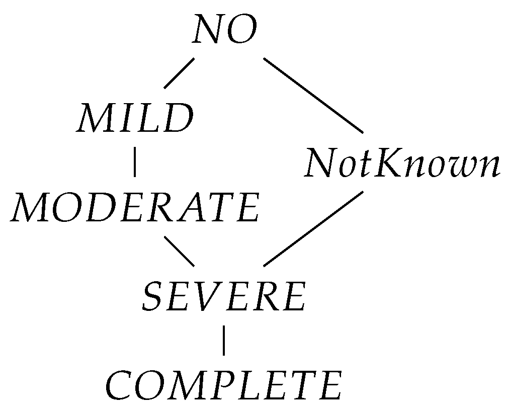
Lattice (m) Nr 13 in Figure 5 then has $NotKnown$ as “optimistically” sidelined with the 5-point scale subchain.

In [11], without graphical representations, there are meet and join tables for all 53 lattices on a 7-point set and all 222 lattices on an 8-point set.

Working with 6-point lattices of the form a “subchain of 5 with one sidelined element” is particularly useful in applications as the 5-point subchain can be viewed as extending the 3-point “traffic light” to a 5-point scale of qualifications together with an element representing “missing data”. Clearly, we may extend the “traffic light” scale in various ways, and as required by the application, keeping in mind that complexity increases and practicability becomes questionable as the number of elements in the lattice grows. Note also that we may pick out more than one sidelined element, with a correspondingly smaller subchain, and provide dedicated interpretations for such elements, i.e., depending on how we prefer to interpret the kind of values they carry. Lattice (b) in Figure 3 can be viewed as a having a 3-point subchain with two sidelined elements. In Figure 4, there are several lattices with more than one sidelined element.

We now proceed with some remarks on semigroups, and we first note that a magma $(X,\ast )$ consists of a set X and a binary operation $\ast :X\times X\to X$, not constrained by any properties whatsoever. A magma is simply a function from $X\times X$ to X.

It is important to understand how the number of structures grow as the number of points in the underlying set increase. In classical boolean logic, there are $2^{2·2}$ = 16 magmas, i.e., binary operations, on a 2-point set. There are $3^{3·3}$ = 19 683 magmas on a 3-point set, $4^{4·4}$ = 4 294 967 296 magmas on a 4-point set, $5^{5·5}$ = 298 023 223 876 953 125 on a 5-point set, and $6^{6·6}$ = 10 314 424 798 490 535 546 171 949 056 magmas on a 6-point set. The set of ${10}^{10·10}$ operators to choose from in a 10-valued logic is obviously more than overwhelming. The situation with $6^{6·6}$ is not as bad as it may seem, as we will see, in particular, when we deal with quantales. Once we require the chosen operators to fulfill certain properties, number 10 314 424 798 490 535 546 171 949 056 becomes downsized to something we can manage, while realizing how it becomes illuminating, conceptually enriching, and, most importantly, applicable.

As we realize how many binary operators, i.e., magmas, we indeed have if nothing whatsoever is required for the operators, we then recognize that the more requirements we add, the less operators we will have. Criteria and constraints involving several operators obviously further increase these numbers.

A semigroup $(X,\ast )$ is a magma where the binary operation $\ast :X\times X\to X$ satisfies $x\ast (y\ast z)=(x\ast y)\ast z$ for all $x,y,z\in X$, i.e., a semigroup is an associative magma.

A semigroup is commutative if $x\ast y=y\ast x$ for all $x,y\in X$, but as we shall see in the case of quantales, we may not always want to require a binary operation to be commutative.

Before discussing quantales, let us recall that arithmetic multiplication is commutative, and this may be the reason why we tend to take the commutative property for granted. However, non-commutative operations are also useful in practice.

We further have to be careful when using arithmetic operation as a basis to construct semigroups in finite sets of numbers, as we see in the following example.

Use ordinary multiplication for the operator $·:\{0,\dots ,5\}\times \{0,\dots ,5\}\to \{0,\dots ,25\}$ to yield

Table 1. Arithmetic multiplication with numbers in $\{0,\dots ,5\}$.

·	0	1	2	3	4	5
0	0	0	0	0	0	0
1	0	1	2	3	4	5
2	0	2	4	6	8	10
3	0	3	6	9	12	15
4	0	4	8	12	16	20
5	0	5	10	15	20	25

.

Now use the rounding $round\left({\displaystyle \frac{a·b}{5}}\right)$ to obtain a binary operator $\ast :\{0,\dots ,5\}\times \{0,\dots ,5\}\to \{0,\dots ,5\}$ to yield the corresponding

Table 2. Binary operation with numbers in $\{0,\dots ,5\}$ based on rounded adaptations.

∗	0	1	2	3	4	5
0	0	0	0	0	0	0
1	0	0	0	1	1	1
2	0	0	1	1	2	2
3	0	1	1	2	2	3
4	0	1	2	2	3	4
5	0	1	2	3	4	5

.

Note that choosing between rounding “point half” values up or down is not relevant in this example as there are no such “point half” values. However natural and practical rounding may be, the resulting operator will not satisfy associativity since, e.g., $(2\ast 2)\ast 3=1\ast 3=1\ne 0=2\ast 1=2\ast (2\ast 3)$, making the operator less appropriate for use in applications.

We now proceed to discuss quantales [9]. A quantale $(X,\ast ,\wedge ,\vee ,\perp ,\top )$ is a semigroup $(X,\ast )$ and a complete lattice $(X,\wedge ,\vee ,\perp ,\top )$, fulfilling the condition that the semigroup operation is join-preserving in both variables, i.e., the following conditions are fulfilled:

$$\begin{array}{cc}\hfill x\ast (\underset{a\in A\subseteq X}{\bigvee }a)& =\underset{a\in A\subseteq X}{\bigvee }(x\ast a)\hfill \\ \hfill (\underset{a\in A\subseteq X}{\bigvee }a)*x& =\underset{a\in A\subseteq X}{\bigvee }(a\ast x)\hfill \end{array}$$

for all $x\in X$ and all $A\subseteq X$.

Note the convention $\bigvee Ø=\perp$, which means that

$$x \ast \perp = \perp \ast x = \perp$$

for all $x\in X$. In some applications this condition may be too restrictive.

Note that a distributive lattice is a quantale with the join as the semigroup operation. However, this is a very special kind of a quantale.

While there are 5 semigroups on a 2-point set, 24 semigroups on a 3-point set, 188 semigroups on a 4-point set, 1915 semigroups on a 5-point set, and 28 634 semigroups on a 6-point set [12], for quantales, there are 2 quantales on a 2-point set, 12 quantales on a 3-point sets, 129 quantales on a 4-point set, 1852 quantales on a 5-point set, and 33 391 quantales on a 6-point set [11].

Table 3. Number of quantales per lattice with 6 elements [11].

Lattice (Nr)	Number of Quantales
1	509
2	2707
3	930
4	1268
5	2157
6	262
7	1547
8	806
9	2972
10	1239
11	2040
12	542
13	2830
14	2253
15	11 329

shows the number of quantales per lattice in the case of 6-point lattices.

A unital quantale $(X,\ast ,e,\wedge ,\vee ,\perp ,\top )$ is a quantale where $(X,\ast ,e)$ is a monoid and where the unit e satisfies

$$x\ast e=e\ast x=x$$

for all $x\in X$. In applications, unital quantales are useful when the sidelined elements are viewed as units.

There are 2830 quantales for the 6-point lattice Nr 13, 57 of which are unital with the sidelined ‘not known’ is the unit. We then have a reasonable condition

$$x\ast NotKnown=NotKnown\ast x=x$$

for all values x in the generic 5-point scale, i.e., computing with unknown values does not affect the overall computation. One of the 57 semigroups, listed as quantale 6.13.1160 in [11] as a unital quantale, is shown in

Table 4. Number of quantales per lattice with 6 elements.

∗	$\mathit{COMPL}$	$\mathit{SEV}$	$\mathit{MOD}$	$\mathit{MILD}$	$\mathit{NO}$	$\mathit{NotKnown}$
$COMPL$	$COMPL$	$COMPL$	$COMPL$	$COMPL$	$COMPL$	$COMPL$
$SEV$	$COMPL$	$COMPL$	$SEV$	$SEV$	$SEV$	$SEV$
$MOD$	$COMPL$	$COMPL$	$MILD$	$MILD$	$MILD$	$MOD$
$MILD$	$COMPL$	$COMPL$	$MILD$	$MILD$	$MILD$	$MILD$
$NO$	$COMPL$	$SEV$	$MILD$	$MILD$	$NO$	$NO$
$NotKnown$	$COMPL$	$SEV$	$MOD$	$MILD$	$NO$	$NotKnown$

.

Note how this semigroup operation in quantale 6.13.1160 is non-commutative. Indeed, we have $SEV\ast MILD=COMPL$, whereas $MILD\ast SEV=SEV$.

In [10], quantales appear under the name cl-semigroup. Inspired by Birkhoff, Goguen’s “L” in L-fuzzy sets is generally a quantale, and such a structure is called a closg for a complete lattice ordered semigroup by Goguen.

We may underline that a completely distributive lattice is indeed a special case of a quantale and the unit interval $[0,1]$ is a very special case of a quantale.

The study of quantales has a long history. Some historical remarks are provided in [9].

4. Fuzzy Sets and Relations of Higher Types

In Section 1, we pointed out how (1) and (2) lead to two different definitions for fuzzy sets of higher types. We can now formulate these alternative definitions using recursive expressions.

If, for the range of fuzzy sets, we write ${\mathbf{R}}_1=[0,1]$ for the type 1 range, we may write ${\mathbf{R}}_2={[0,1]}^{{\mathbf{R}}_1}$, or alternatively, ${\mathbf{R}}_2={{\mathbf{R}}_1}^{[0,1]}$, for the type 2 range. In both cases, ${\mathbf{R}}_2={[0,1]}^{[0,1]}$, i.e., for type 2 fuzzy sets we have only one definition.

The alternative definitions become apparent when we generally have

$${\mathbf{R}}_n={[0,1]}^{{\mathbf{R}}_{n-1}}$$

(7)

or, alternatively,

$${\mathbf{R}}_n={{\mathbf{R}}_{n-1}}^{[0,1]}$$

(8)

for the type n range, $n=2,3,\dots$.

The set of fuzzy sets of type n over a set X is thus

$${{\mathbf{R}}_n}^X={\left({[0,1]}^{{\mathbf{R}}_{n-1}}\right)}^X$$

(9)

or, alternatively

$${{\mathbf{R}}_n}^X={\left({{\mathbf{R}}_{n-1}}^{[0,1]}\right)}^X$$

(10)

Goguen [4] wrote intuitively about “fuzzy fuzzy sets of X” and how “there is no end to the possible levels of fuzzification”. He further remarked on the difference between $X^{\left(Y^Z\right)}$ and ${\left(X^Y\right)}^Z$, and preferred (Goguen in [4] writes that “when we write ${X^Y}^Z$, we shall intend the stronger form $X^{\left(Y^Z\right)}$”) to use $X^{\left(Y^Z\right)}$, which corresponds to alternative (9), with the simple argument that L, the lattice of fuzzy values, appears in the base of the powerset $L^X$ of L-fuzzy sets over X. Goguen did not, however, provide practical examples to justify their preference.

As we now realize that there are indeed alternative ways to define higher types of fuzzy sets, we are obviously interested in comparing notations used for fuzzy sets of higher types, respectively, e.g., in [1,2,13,14,15,16,17,18], and indeed, in order to identify which alternative interpretation is preferred.

Before comparing notations, let us see how the set and function representations of fuzzy sets play out in the respective alternative definitions of fuzzy sets of higher types. In order to make expressions more transparent, we will use Q instead of the unit interval [0,1], and we will first distinguish between Q appearing as base and the exponent in $Q^Q$ by using $Q_b$ for the base and $Q_e$ for the exponent. Note that, indeed, $Q_b$ and $Q_e$ need not necessarily represent one and the same algebraic structure for the set of membership values, but for the purpose of seeing how set and function representations of fuzzy sets play out, we need not prescribe whether or not $Q_b$ and $Q_e$ represent the same structure. In fact, Zadeh in [1,2] introduced the higher types by first describing the situation for $Q_b=\{0,1\}$.

The range of fuzzy sets of type 2 is thus

$${Q_b}^{Q_e}$$

(11)

and the range for fuzzy sets of type n, $n=2,3,\dots$, is

$${\mathbf{R}}_{e,n}={Q_b}^{{\mathbf{R}}_{e,n-1}}$$

(12)

with ${\mathbf{R}}_{e,1}=Q_e$, or, alternatively,

$${\mathbf{R}}_{b,n}={{\mathbf{R}}_{b,n-1}}^{Q_e}$$

(13)

with ${\mathbf{R}}_{b,1}=Q_b$.

Note that if $Q_b$ is a quantale, then so is ${\mathbf{R}}_{e,n}$ and ${\mathbf{R}}_{b,n}$.

The set of fuzzy sets of type n over a set X is thus

$${{\mathbf{R}}_{e,n}}^X={\left({Q_b}^{{\mathbf{R}}_{e,n-1}}\right)}^X$$

(14)

or, alternatively,

$${{\mathbf{R}}_{b,n}}^X={\left({{\mathbf{R}}_{b,n-1}}^{Q_e}\right)}^X$$

(15)

Note how these recursive expressions make use of only $Q_b$ and $Q_e$. For instance, for n = 4, (12) and (13) become, respectively,

$${\mathbf{R}}_{e,4}={Q_b}^{\left({Q_b}^{\left({Q_b}^{Q_e}\right)}\right)}$$

and

$${\mathbf{R}}_{b,4}={\left({\left({Q_b}^{Q_e}\right)}^{Q_e}\right)}^{Q_e}$$

Obviously, once the range for a fuzzy set of a selected type n has been determined by one of the alternatives, different algebraic structures $Q_i$, $i=1,\dots ,n$, may be used in the recursive definitions, and we then obtain the following definitions for the range of fuzzy sets of type n, $n=2,3,\dots$

$${\mathbf{R}}_{e,n}={Q_n}^{{\mathbf{R}}_{e,n-1}}$$

(16)

with ${\mathbf{R}}_{e,1}=Q_1$, or, alternatively,

$${\mathbf{R}}_{b,n}={{\mathbf{R}}_{b,n-1}}^{Q_n}$$

(17)

with ${\mathbf{R}}_{b,1}=Q_1$, and the definition of the set of fuzzy sets of type n over a set X is

$${{\mathbf{R}}_{e,n}}^X={\left({Q_n}^{{\mathbf{R}}_{e,n-1}}\right)}^X$$

(18)

or, alternatively,

$${{\mathbf{R}}_{b,n}}^X={\left({{\mathbf{R}}_{b,n-1}}^{Q_n}\right)}^X$$

(19)

Now these recursive expressions make use of a wider variety of structures. For instance, for n=4, (16) and (17) become, respectively,

$${\mathbf{R}}_{e,4}={Q_4}^{\left({Q_3}^{\left({Q_2}^{Q_1}\right)}\right)}$$

and

$${\mathbf{R}}_{b,4}={\left({\left({Q_1}^{Q_2}\right)}^{Q_3}\right)}^{Q_4}$$

Note that the algebraic structure of both ${{\mathbf{R}}_{e,n}}^X$ and ${{\mathbf{R}}_{b,n}}^X$ is inherited solely from the algebraic structure of its base without any “algebraic involvement” of X. In the set $Q^X$ of fuzzy sets of type 1, the algebraic operations in $Q^X$ are inherited from Q. For instance, a join operation ${\wedge }_Q$ in Q, which for element $x_1,x_2\in Q$ provides $x_1{\wedge }_Q{x}_2$ in Q, is used to define a corresponding join operation ${\wedge }_{Q^X}$ in $Q^X$, so that for any fuzzy sets ${\mu }_1,{\mu }_2:X\to Q$ and any $x\in X$, we have

$$\left({\mu }_1{\wedge }_{Q^X}{\mu }_2\right)\left(x\right)={\mu }_1\left(x_1\right){\wedge }_Q{\mu }_2\left(x_2\right)$$

In the case of type 2 fuzzy sets, the algebraic structure of ${\left({Q_b}^{Q_e}\right)}^X$ is then inherited solely from the algebraic structure of ${Q_b}^{Q_e}$, but it is an open question what the algebraic structure of ${Q_b}^{Q_e}$ actually is. It may in turn inherit its algebraic structure solely from $Q_b$, in particular, if and when ${Q_b}^{Q_e}$ is viewed as a set of fuzzy sets. In this case, the algebraic structure of $Q_e$ is indeed ignored. This ignorance is justified if for type 2 fuzzy sets we have the underlying idea that “the membership value is a fuzzy set”. Then ${Q_b}^{Q_e}$ is viewed as a set of fuzzy sets, and then the structure of $Q_e$ is ignored. On the other hand, if we say “the membership value is fuzzy”, or, “the membership value is a higher type of membership value”, then ${Q_b}^{Q_e}$ can be viewed as something other than just a set of fuzzy sets. For instance, if ${Q_b}^{Q_e}$ is taken not as the set of all functions from $Q_e$ to $Q_b$ but instead as the set of all join-preserving algebra homomorphisms, $Q_e$ to $Q_b$, then the set ${Q_b}^{Q_e}$ is different, and so is its algebraic structure. Join preservation means that a function $f:Q_e\to Q_b$, in the finite case, fulfills the condition

$$f\left(x_1{\vee }_e{x}_2\right)=f\left(x_1\right){\vee }_{b}f\left(x_2\right)$$

where ${\vee }_e$ and ${\vee }_b$ are the join operations, respectively, in $Q_e$ and $Q_b$. For example, if $Q_e$ and $Q_b$ are the same and taking a 3-point quantale Q over the 3-point lattice as a chain, then the set and lattice of join-preserving functions, often written $[Q,Q]$ and not to be confused with the base structure ignoring power $Q^Q$, will have lattice (k) Nr 11, shown in Figure 4, as its underlying lattice.

The set and lattice $[Q,Q]$ equipped with function composition as a semigroup operation makes $[Q,Q]$ a quantale.

In the infinite case we have the corresponding condition

$$f(\bigvee A)=\underset{x\in A}{\bigvee }f\left(x\right)$$

It is important to underline the distinction between $Q^Q$ as a structure, ignoring power from $[Q,Q]$ as the set of join-preserving functions, simply from the viewpoint of the numbers of elements in respective sets. In $Q^Q$, where the base Q is viewed as a quantale and the power Q as just a set, the number of fuzzy sets over Q, the domain, equals $3^3$, i.e., 27, and as the size of Q grows, the number of fuzzy sets in

$$Q^{\left(Q{\dots }^{\left(Q^Q\right)\dots }\right)}$$

is incomprehensible. On the other hand, and for fuzzy sets of type n, with n being smaller, and many of the quantales $Q_1,\dots ,Q_n$ in

$${Q_n}^{\left(Q_{n-1}{\dots }^{\left({Q_2}^{Q_1}\right)\dots }\right)}$$

being small—some even being 2-pointed or 3-pointed, for whatever reason provided in applications—the number of elements as functions is much smaller and also classifiable by algebraic properties.

Going beyond 2 to higher types of fuzzy sets means that the “structure ignorance” will be differently located depending on whether we prefer to use ${\mathbf{R}}_{b,n}$ or ${\mathbf{R}}_{e,n}$. In this paper, we do not dwell in more detail on the join-preserving functions. The situation on 3-point quantales is discussed in [19].

It is also important to observe some detail concerning the set representation of higher-type fuzzy sets. Given a fuzzy set of type 2

$$\mu :X\to {Q_b}^{Q_e},$$

we now obtain the set representation as a subset

$$A_{\mu }\subseteq X\times {Q_b}^{Q_e}$$

given by

$$A_{\mu }=\{(x,\mu \left(x\right))\mid x\in X,\mu \left(x\right):Q_e\to Q_b\}$$

(20)

Because of Cartesian closedness, we will have

$${\left({Q_b}^{Q_e}\right)}^X\cong {Q_b}^{X\times Q_e}$$

and $\mu$ will therefore produce

$${\mu }^{♮}:X\times Q_e\to Q_b,$$

defined by ${\mu }^{♮}(x,\alpha )=\mu \left(x\right)\left(\alpha \right)$, with a corresponding set representation as a subset

$$A_{{\mu }^{♮}}\subseteq (X\times Q_e)\times Q_b$$

given by

$$A_{{\mu }^{♮}}=\{((x,\alpha ),{\mu }^{♮}(x,\alpha ))\mid (x,\alpha )\in X\times Q_e,{\mu }^{♮}:X\times Q_e\to Q_b\}$$

(21)

which can also be written as

$$A_{{\mu }^{♮}}=\{((x,\alpha ),\beta )\mid (x,\alpha )\in X\times Q_e,\beta ={\mu }^{♮}(x,\alpha )\in Q_b\}$$

(22)

The generalization to type n is now as follows and is indeed in the “structure ignorance” situation. Alternative (18) unfolds as

$${\left({Q_n}^{{\mathbf{R}}_{e,n-1}}\right)}^X\cong {Q_n}^{X\times {\mathbf{R}}_{e,n-1}}={Q_n}^{X\times {Q_{n-1}}^{{\mathbf{R}}_{e,n-2}}}={Q_n}^{X\times {Q_{n-1}}^{\left({Q_{n-2}}^{{\mathbf{R}}_{e,n-3}}\right)}}=...$$

(23)

which gives the congruence

$${\left({Q_n}^{{\mathbf{R}}_{e,n-1}}\right)}^X\cong {Q_n}^{X\times {Q_{n-1}}^{\left(Q_{n-2}{\dots }^{\left({Q_2}^{Q_1}\right)\dots }\right)}},$$

(24)

and alternative (19) unfolds as

$${\left({{\mathbf{R}}_{b,n-1}}^{Q_n}\right)}^X\cong {{\mathbf{R}}_{b,n-1}}^{X\times Q_n}\cong \dots \cong {Q_1}^{(\dots (((X\times Q_n)\times Q_{n-1})\times Q_{n-2})\times \dots )\times Q_2}$$

(25)

providing the congruence

$${\left({{\mathbf{R}}_{b,n-1}}^{Q_n}\right)}^X\cong {Q_1}^{X\times \left({\Pi }_{i=0}^{n-2}{Q}_{n-i}\right)}$$

(26)

Note how congruences (24) and (26) show that a fuzzy set of type n can in fact be viewed as congruent with a fuzzy set of type 2, but with quite different views of reductions with respect to what happens in the exponent.

The set representation of (24) is now

$$A_{{\mu }^{♮}}=\{((x,\varphi ),\beta )\mid (x,\varphi )\in X\times {Q_{n-1}}^{\left(Q_{n-2}{\dots }^{\left({Q_2}^{Q_1}\right)\dots }\right)},\beta ={\mu }^{♮}(x,\varphi )\in Q_n\},$$

(27)

where

$$\varphi :\left(Q_{n-2}{\dots }^{\left({Q_2}^{Q_1}\right)\dots }\right)\to Q_{n-1}$$

is a function, and the set representation of (26) is

$$A_{{\mu }^{♮}}=\{((x,\overline{\alpha }),\beta )\mid (x,\overline{\alpha })\in X\times \left({\Pi }_{i=0}^{n-2}{Q}_{n-i}\right),\beta ={\mu }^{♮}(x,\overline{\alpha })\in Q_1\}$$

(28)

where $\overline{\alpha }\in {\Pi }_{i=0}^{n-2}{Q}_{n-i}$ is an $n-1$-tuple.

Note in both (27) and (28) how the data structures in the exponent cannot detach any substructure that is not connected with an element x in X. In other words, when in [1,2] Zadeh says “membership values are allowed to be fuzzy set”,we should understand it as “membership values connected with elements x in X are allowed to be fuzzy sets”.

We have now arrived at a key point of this paper, namely, that, concerning the intuitive idea for “fuzzy fuzzy”, we are in position to distinguish between “a fuzzy set is fuzzy”, as defined by (9), and “fuzzy is a fuzzy set”, defined by (10).

Now we are in a position to go into detail concerning the comparison of notations used for fuzzy sets of higher types in [1,2], [13,14], [15,16], and [17,18].

Zadeh’s “point of departure” in [1,2] to understand operations on fuzzy sets of type 2 is to start with type 2 fuzzy sets of form

$$\mu :X\to {\{0,1\}}^{[0,1]}$$

(29)

and further restricting $\mu \left(x\right)$ to be a subinterval of the interval $[0,1]$. This enables Zadeh to use level sets and convex fuzzy sets of type 1 in order to arrive at a definition for intersections of fuzzy sets of type 2. In [1,2], Zadeh indeed defines a fuzzy set of type n, $n=2,3,\dots$, to have its membership function ranging over fuzzy sets of type $n-1$, but Zadeh does not provide the recursive definition, and he also provides no detail beyond that for fuzzy sets of type 2, so one cannot say how [1,2] intended to view fuzzy sets of higher types from the viewpoint of (9) and (10).

Mizumoto and Tanaka [13] defined fuzzy sets of type 2 as

$${\mu }_A:X\to {[0,1]}^J,$$

saying that J may be the unit interval or a subset thereof, or even a finite subset of the unit interval. “By analogy”, they say fuzzy sets of type n can be defined as

$${\mu }_A:X\to {{{[0,1]}^{J_1}}^{⋰}}^{J_{n-1}},$$

(30)

where $J_1,\dots ,J_{n-1}$ are subsets of $[0,1]$. Using a set X like $\{x_1,x_2,x_3\}$, and a fuzzy set A is expressed as

$$A=low/x_1+middle/x_2+high/x_3$$

The fuzzy grades $low$, $middle$, and $high$ are said to be fuzzy sets over $J=\{0,0.1,\dots ,0.9,1\}$, with, for instance, $low$ expressed as

$$low=1/0+0.9/0.1+0.7/0.2+0.4/0.3$$

Further, $notlow$ is defined as

$$notlow=0.1/0.1+0.3/0.2+0.6/0.3+1/(0.4+0.5\dots +1)$$

As we have remarked before, Zadeh’s summation notation of fuzzy sets may be misused and the subexpression “$1/(0.4+0.5\dots +1)$” is certainly not within the realm of intended use in the summation notation, even if a reader most probably will understand it “correctly”. Clearly, that subexpression is intended as an abbreviation for “$1/0.4+1/0.5+\dots +1/1$”.

We can see how A is the fuzzy set $A:X\to {[0,1]}^J$, and $A\left(x_1\right)=low$. Further, $low$ is intended to be the fuzzy set $low:J\to [0,1]$, even if $low$ is defined as $low:J\to J$. Mizumoto and Tanaka then proceeds to provide a wide range of properties for fuzzy sets of type 2, but the paper does not contain any further remarks on fuzzy sets beyond type 2. It is therefore unclear how [13] would understand (30) from the viewpoint of being either of form (9) or (10).

As Hisdal points out in [15], Zadeh introduced fuzzy sets of higher types informally in [20]. Hisdal then states that fuzzy sets of higher type “were defined by them exactly in ([2] definition 3.1)”. We may not agree perfectly with Hisdal’s “exactly”, and indeed, Hisdal’s own re-definition is formulated in the same style and with basically the same content as Zadeh’s definition. Hisdal’s (3.2.2) in subSection 3.2 is according to (10), and generally in accordance with (15), as unfolded by Cartesian closedness in (25), which is confirmed in her subSection 3.3. Hisdal in her “numerical representation” of a fuzzy set of type n says that type n fuzzy sets reduce to being fuzzy sets of type 1, since she writes her “N-dimensional universe” as

$$V\times M^{t1}\times M^{t2}\times \dots \times M^{t(N-1)}$$

where $M^{tn}$, as Hisdal says, “may be the interval $[0,1]$ or a subset of this interval”.

In [16] we see a variation of (22) using the following set representation to define fuzzy sets of type 2:

$$A_{{\mu }^{♮}}=\{((x,\alpha ),{\mu }^{♮}(x,\alpha ))\mid x\in X,\alpha \in J_x\subseteq [0,1]\}$$

(31)

From a formal point of view, the use of the index ‘x’ in the set $J_x$ is superfluous. Finite subsets $J_i$ of membership values in $[0,1]$ seems in [13] to be used to indicate that the elements in $J_i$ are the only ones “used in practice”. The use of $J_x$ in [16] is adopted also because it supports graphical representations, i.e., so that

$$J_x=\{\alpha \in [0,1]\mid {\mu }^{♮}(x,\alpha )>0\}$$

Fuzzy sets of type higher than 2 do not appear in [16], and obviously, the “shading technique” works well in graphical representation for type 2 fuzzy sets.

These graphical representation styles are in [21] extended to horizontal and vertical “type 3 slicing techniques” for fuzzy sets of type 3.

A state-of-the-art definition of type 3 fuzzy sets can be found, e.g., in [17,18,22]. A type 3 fuzzy set is defined as a trivariate function

$$\mu :X\times [0,1]\times [0,1]\to [0,1]$$

i.e., in accordance with (26) for $n=3$ where $Q_1=Q_2=Q_3=[0,1]$. The set representation of $\mu$ is

$$A_{{\mu }^{♮}}=\{((x,u,v),\mu (x,u,v))\mid (x,u,v)\in X\times [0,1]\times [0,1]\}$$

i.e., in accordance with (28).

In [22] there is broader treatment of notations, but still overlooking the two alternatives, and indeed in the type n definition favouring the alternative that was promoted already by Hisdal in 1981.

Clearly, when there is a desire to present higher-type fuzzy sets graphically, certain data structures need to be introduced in order to manage the many-dimensionality of the surfaces representing the higher-type fuzzy set. Notational clarifications as presented, e.g., in [22], certainly support graphical representations of higher-order fuzzy sets, but in this paper we still do not see that these clarifications provide the precise recursive definition that indeed reveals that there are alternative understandings of the “Mizumoto power expression”.

5. Fuzzy Sets of Higher Types in Design Structure Matrices

As an application of quantales for fuzzy sets and relations of higher types we will look at the design structure matrix (DSM), originally presented in [23]. The DSM can be viewed as a many-valued relation where the positions in the matrix may have different dedicated sets of qualifications [24]. DSMs have been used in a variety of applications [25]. Many-valued and many-sorted aspects of DSMs were presented in [26].

A two-valued DSM is a relation $R\subseteq X\times X$ on a domain as a finite set $X=\{e_1,\dots ,e_n\}$ of labels. Related elements $e_i$ and $e_j$, $e_{i}R{e}_j$, are said to interact, where interaction is directed, i.e., a DSM relation is typically not symmetric.

Basic DSM domains are those for Components, People, and Activities, for which label sets can be denoted, respectively, by $X_{Co}$, $X_{Pe}$, and $X_{Ac}$. Examples are drawn mostly from the manufacturing industry where the domains are combined in multidomain matrices (MDM).

A many-valued DSM viewed in its function representation $f:X\times X\to Y$ makes use of a set Y of attributes or qualifications, and Y often includes the algebraic structure, e.g., being an ordered set of qualifications or enabling operation with attributes.

A DSM is in applications graphically presented as a table with rows and columns, and it is often viewed as a square n-by-n matrix as defined in linear algebra, which in turn invites to understand calculations based on matrix manipulation as in linear algebra. However, a relational view of a DSM similarly invites using relational algebra for computing with many-valued relations $f:X\times X\to Y$.

A two-valued DSM may use the check mark “✓” to indicate that two elements are related. A DSM empty cell means that two elements are not related, and then Y may be given as $\{0,1\}$ or $\{0,✓\}$, or similar. However, Y can be any type of a set, structured or unstructured.

A relation in DSM

$$\delta :X\times X\to Q$$

represents a fuzzy relation of type 1, and can be seen as a fuzzy set of type 1, where the domain of $\delta$ is the product $X\times X$. This view of a DSM can immediately be extended to fuzzy relations of type n as

$$\rho :(X\times X)\times Q^{n-1}\to Q$$

according to alternative (24), i.e., for any $x_1,x_2\in X$, we obtain fuzzy sets

$${\tilde{\rho }}_{x_1,x_2}:Q^{n-1}\to Q$$

In the case of multiple domains $X_{d_1},\dots ,X_{d_m}$, a fuzzy set of type n can then be represented as

$$\tilde{\delta }:X_{d_1}\times \dots \times X_{d_m}\to Q^{Q^{n-1}}$$

In [26] we described a fuzzy set model for the “documentation of interaction between elements”, described in [27] using the set

$$\{Detrimental,Undesired,Indifferent,Desired,Required\}$$

to represent a scale set $\{-2,-1,0,1,2\}$ of scores, respectively, for $Spatial$, $Energy$, $Information$, and $Materials$. We may now set

$$J_i=\{-2,-1,0,1,2\},i=Spatial,Energy,Information,Materials$$

and obtain a DSM as

$$\delta :X\times X\to J_{Spatial}\times J_{Energy}\times J_{Information}\times J_{Materials}$$

whenever we are certain about the qualification of the relation between two elements in a DSM domain. A corresponding uncertain qualification may then be represented as

$$\tilde{\delta }:X\times X\to Q^{J_{Spatial}\times J_{Energy}\times J_{Information}\times J_{Materials}}$$

which is a fuzzy set of type 5.

We may also note how an MDM needs to relate, or “map” elements between domains. If elements in Y are symbols in the form of numbers, it invites application developers to compute with numbers, even if elements in Y might be closer to be interpretable as truth values or “membership grades” in a many-valued setting. If, on the other hand, elements in Y are understood as being non-numerical symbols, and Y is equipped with an algebraic structure, then it invites computation with these symbols algebraically.

6. Logic with Fuzzy or Fuzzy Logic

For a Q-fuzzy set $\mu :X\to Q$ we have so far discussed structure only concerning the range Q, leaving the domain X as it is, namely, a set of points, but obviously, the domain X is also equipped with structure, at least potentially, and it is often much more complicated than the structure of Q. However, fuzzy set theory in its starting point makes no assumptions nor proposals whatsoever concerning the structure of the domain X. This was pointed out also by Goguen [4], saying “X generally has some structure beyond that of a set”, but then also saying that their notion of L-fuzzy sets makes no assumption about the structure on X. Goguen spoke generally about examples using vector and Hilbert spaces as structures on X, and he also mentioned topological and metric spaces to capture concepts of “nearness” in X. Goguen’s suggestions are certainly reasonable and justifiable, and they should be explored.

In this section, with a focus on logic, we suggest to focus more on elements in X as being “expressions” in the form of terms created by some underlying signature of sorts and operators, as we typically do in first-order logic.

Elements in X being terms means that X is a “set of terms”, which we informally may denote as “$TX$”, with T being a constructor along with the powerset constructor $\mathsf{P}$ and the fuzzy powerset constructor $\mathsf{Q}$. Note, however, the fundamental difference, as “$TX$” is informally a “set of terms”, whereas $\mathsf{Q}X$ is the set of Q-fuzzy sets over X, where X is a set of elements, i.e., X is unstructured.

Now note, still informally, that we may and even should be curious about “fuzzy sets over $TX$”, i.e., fuzzy sets where we provide membership values to expressions rather than simply to elements.

This curiosity was the starting point for developing the notion of “fuzzy terms” [28], and in this section, we give a brief overview on how to make the notion of the “term constructor” T more precise and on how we formally “compose” the constructors $\mathsf{Q}$ and T in order to arrive at fuzzy terms.

Before going into detail, we should be aware that uncertainty of terms can be introduced in different ways, so that we can make a distinction between “logic with fuzzy” and “fuzzy logic”, depending on whether logical expressions are constructed over the ordinary category of sets and functions or the category of fuzzy sets and fuzzy morphisms [4].

In order to explain this distinction more formally, let us begin with a simple example involving the expression “$2+3$”. Both “2” and “3” may be uncertain and represented by fuzzy sets, so that the fuzzy set of “$2+3$” can be constructed, e.g., using the extension principle applied to real number addition. This indeed creates a “fuzzy addition”, based on the original addition on the real line, but we should note that in this case the original addition itself is not considered to be uncertain.

In order to illuminate uncertainty of operation, let us take a folding meter stick, i.e., a carpenter’s ruler, one meter long. The “operation” of producing “one more metre” can be repeated, e.g., when measuring the length of a field of play in football. While walking across the field, producing “metre operations” one by one in sequence, an error will accumulate, but not because “1” is fuzzy, but indeed because the stick that produces “1” is fuzzy. Similarly, if an addition “$2+3$” is uncertain, it may not necessarily be “2” or “3” to blame, but the uncertainty may in fact reside in the operation “+”.

Here we indeed intuitively realize how there is a fundamental distinction between “computing with fuzzy”, where the operation “+” is certain while “2” and “3” are uncertain, and “fuzzy computing”, where “+” may be uncertain while “2” and “3” are certain. Within the fuzzy community and the fuzzy literature, what is frequently called “fuzzy computing” is in fact in the style of “computing with fuzzy”, i.e., not allowing the operators themselves to be uncertain than as non-fuzzy operators by the extension principle, providing a corresponding “fuzzy operator” enabled to operate with fuzzy objects.

The formal explanation of the distinction is suitably explained using the language of category theory. A primer of category theory for “fuzzy terms” is found in [28], and treatments of category theory in general can be found in many textbooks, e.g., in [29] or [30].

The powerset of all subsets of X can be seen as coming from the powerset functor$\mathsf{P}:\mathtt{Set}\to \mathtt{Set}$. For a set X, i.e., an object in $\mathtt{Set}$, $\mathsf{P}X$ is the powerset of X. We may now, for a quantale Q, introduce the functor $\mathsf{Q}:\mathtt{Set}\to \mathtt{Set}$, where $\mathsf{Q}X$ is $Q^X$, i.e., the set of all Q-fuzzy sets over X.

Fuzzy terms are in [28] introduced using a formal term functor construction first for ordinary terms over a signature $\Sigma =(S,\Omega )$, consisting of a set S of sorts (or types) and a set $\Omega$ of operators. The term functor

$${\mathsf{T}}_{\Sigma }:{\mathtt{Set}}_S\to {\mathtt{Set}}_S$$

over the sorted category ${\mathtt{Set}}_S$, produces terms over $\Sigma$ using variables in a sorted set $X_S={\left(X_{\mathtt{s}}\right)}_{\mathtt{s}\in S}$. The sorted set ${\mathsf{T}}_{\Sigma }{X}_S$ of terms contains all terms constructed using operators in $\Omega$ and the variables in the sorted set $X_S$. Note indeed that the “set of all terms” is the sorted set

$${\mathsf{T}}_{\Sigma }{X}_S={\left({\mathsf{T}}_{\Sigma ,\mathtt{s}}{X}_S\right)}_{\mathtt{s}\in S}$$

and we may therefore consider fuzzy sets

$${\mu }_{\mathtt{s}\in S}:{\mathsf{T}}_{\Sigma ,\mathtt{s}}{X}_S\to {\mathbf{R}}_{\square ,n}$$

over ${\mathsf{T}}_{\Sigma ,\mathtt{s}}{X}_S$, separately for each $\mathtt{s}\in S$, where ${\mathbf{R}}_{\square ,n}$ is either ${\mathbf{R}}_{e,n}$ or ${\mathbf{R}}_{b,n}$, potentially also with quantales in ${\mathbf{R}}_{\square ,n}$, provided specifically for each $\mathtt{s}\in S$, thus opening up a very wide spectrum of alternatives for application development.

See [28] for full details concerning the categorical term construction over multisorted signatures.

Note indeed how “variables” must respect the sorts, so that we have variables of type $s\in S$. If the sort set contains connected sorts, e.g., with truth values and numbers, we have to separate “variables for truth values” from “variables for numbers”. Note also that variables themselves are terms.

Returning to the informal view on “set of terms” with the informal notation $TX$, we are immediately tempted to explore applications involving fuzzy sets like $\mu :TX\to Q$. This essentially means we are in position to replace X with $TX$ in (18) and (19). We also immediately see how $Q^{TX}$ is the same as $QTX$, i.e., coming from the composed functor $\mathsf{Q}\circ \mathsf{T}$. In the many-sorted case, (18) and (19) have to be treated using sorted sets, details of which are outside the scope of this section.

Working with X just as a set of elements is similarly adopted in probability theory, where a set of “samples” is just a set of elements, even if “sample” may have an intuitive meaning and potential structure, as pointed out already by Kolmogorov [31]. Probability theory often speaks about the “event space”, where an “event” is a subset of “samples”, and the “space” structure is that of a $\sigma$-algebra.

In the following we recall some rudimentary examples of signatures used in [28].

A signature for natural numbers, or “Peano numbers”, is typically given by $\mathtt{NAT}=\left(\right\{\mathtt{nat}\},\{\mathtt{0}:\to \mathtt{nat},\mathtt{succ}:\mathtt{nat}\to \mathtt{nat}\left\}\right)$, which indeed is a fundamental example syntactically producing the natural numbers. This signature could be extended, e.g., with an operator for addition. The term set ${\mathsf{T}}_{\mathtt{NAT}}Ø$ consists of the “Peano numbers” $\mathtt{0},\mathtt{succ}\left(\mathtt{0}\right),\mathtt{succ}\left(\mathtt{succ}\right(\mathtt{0}\left)\right),\dots$.

The signature for boolean truth values is given by $\mathtt{BOOL}=\left(\right\{\mathtt{bool}\},\Omega )$, with $\Omega$ containing the constants $\mathtt{false}:\to \mathtt{bool},\mathtt{true}:\to \mathtt{bool}$, together with additional binary operators, like for “AND” we would add the meet operation $\wedge :\mathtt{bool}\times \mathtt{bool}\to \mathtt{bool}$. The sorted set of variables is now just a single set X since the sort set in the signature consists of only one element. The term set ${\mathsf{T}}_{\mathtt{BOOL}}X$ consists of expressions (terms) like x, $\mathtt{true}$, $\wedge (x_1,\mathtt{true})$, $\wedge (\wedge (x_2,\mathtt{false}),\mathtt{true})$, and so on, with $x,x_1,x_2\in X$.

A signature $\mathtt{NATORD}=\left(\right\{\mathtt{nat},\mathtt{bool}\},\{\mathtt{0}:\to \mathtt{nat},\mathtt{succ}:\mathtt{nat}\to \mathtt{nat},\mathtt{false}:\to \mathtt{bool},\mathtt{true}:\to \mathtt{bool},\le :\mathtt{nat}\times \mathtt{nat}\to \mathtt{bool}\left\}\right)$, can be introduced as a many-sorted situation where the operator ≤ needs both $\mathtt{nat}$ and $\mathtt{bool}$. Again, this signature can be extended, e.g., to $\mathtt{NATADDORD}$, by adding the operator $+:\mathtt{nat}\times \mathtt{nat}\to \mathtt{nat}$ (reserved for addition, but still semantically or equationally undefined) to the set of operators in $\mathtt{NATORD}$. Similarly, logical operators could be included, and so on.

Computing with fuzzy now corresponds to the functor composition, informally written as

$$\mathsf{Q}\circ \mathsf{T}:\mathtt{Set}\to \mathtt{Set}$$

where we need to work with sorted categories. The composition can be extended to a monad composition $\mathbf{Q}\circ \mathbf{T}$, which enables variable substitution to work as expected, i.e., substitutions can be composed [28].

Note that a variable substitution involving ordinary terms is, informally written, a function $\sigma :X\to \mathsf{T}X$. In the $\mathtt{NAT}$ signature, the term $\wedge (\wedge (x_2,\mathtt{false}),\mathtt{true})$ can be seen as the result of a substitution, where $\wedge (x_2,\mathtt{false})$ has been substituted into $x_1$ in $\wedge (x_1,\mathtt{true})$. Strictly speaking, when variables for terms in “$\mathsf{T}X$” are substituted by terms, we will end up with terms in “$\mathsf{T}\mathsf{T}X$”, but because of the impotency “$\mathsf{T}$$\mathsf{T}$X=$\mathsf{T}$X”, all “terms over terms” are still “just terms”.

Variable substitution works perfectly well [28] also for terms in “$\mathsf{Q}$$\mathsf{T}$X”, using the multiplication of the monad as kind of a “flattening operator”, so that variable substitution using “fuzzy sets of terms” can be managed. A variable substitution in this case is (informally) a function

$$\sigma :X\to \mathsf{Q}\mathsf{T}X$$

and now, in composition of substitutions, we cannot rely on idempotency, since “fuzzy terms over fuzzy terms” are not simply “just fuzzy terms”. Substitution leads to terms residing in $\mathsf{Q}\mathsf{T}\mathsf{Q}\mathsf{T}X$, which requires having a “flattening” transformation, categorically a natural transformation as a multiplication in the corresponding composed monad $\mathbf{Q}$$\mathbf{T}$ between the functor compositions $\mathsf{Q}\mathsf{T}\mathsf{Q}\mathsf{T}$ and $\mathsf{Q}\mathsf{T}$.

Fuzzy computing, on the other hand, corresponds to the term functor over the Goguen category, i.e., informally written as

$$\mathsf{T}:\mathtt{Set}\left(Q\right)\to \mathtt{Set}\left(Q\right)$$

where we similarly need to work with sorted categories. See [28] for full details concerning the categorical term construction over Goguen categories. It is needless to say variable substitution in “fuzzy computing” is quite complicated but indeed perfectly manageable.

Computing with fuzzy and fuzzy computing shows how we are moving away from working just with sets of points to working with sets of expressions, and, again intuitively said, with fuzzy sets of expressions not to be confused with sets of fuzzy expressions.

Generally speaking, logic is a structure and indeed a very complicated one. Logic as a structure contains signatures, terms, sentences (formulae), structured sets of sentences, entailment, semantics (universal algebra), satisfaction, axioms, theories and proof calculi, so fuzzy logic, also as a structure, and a many-valued structure, potentially contains fuzzifications but not trivial ones, of all parts of logic, i.e., we potentially have fuzzy signatures, fuzzy terms, fuzzy sentences, fuzzy structured fuzzy sets of fuzzy sentences, fuzzy entailment, fuzzy algebra, fuzzy satisfaction, fuzzy axiom, fuzzy theories, and fuzzy proof calculi.

Depending on our choice concerning construction of “fuzzy terms” we will end up either working with “logic with fuzzy”, i.e., using fuzzy sets of ordinary terms as the basis for the logic, or working with “fuzzy logic”, i.e., using fuzzy terms over $\mathtt{Set}\left(Q\right)$ as a basis for logical expressions where operators in the signature are allowed to be uncertain.

The overall framework, still not fully developed in all parts, is explained in [32,33].

We conclude this section with the remark that the underlying algebraic structure for membership values in the Goguen category

$$\mathtt{Set}\left(Q\right)$$

can be provided also in Goguen categories

$$\mathtt{Set}\left({\mathbf{R}}_{\square ,n}\right)$$

using fuzzy sets of higher type.

7. Summary, Conclusions, and Future Work

For fuzzy sets of higher type we have proposed to include structure in both the domain and range of fuzzy sets

$${\mu }_{\mathtt{s}\in S}:{\mathsf{T}}_{\Sigma ,\mathtt{s}}{X}_S\to {\mathbf{R}}_{\square ,n}$$

(32)

as compared to fuzzy sets having no structure in the domain and the range using the unit interval

$$\mu :X\to [0,1]$$

as proposed in [3] for fuzzy sets of type 1, and similarly for fuzzy sets of type 2 in [1,2] according to

$$\mu :X\to {[0,1]}^{[0,1]}$$

based on which the extension to fuzzy sets of type n was proposed but rather informally, and with informally represented power expressions, in [13].

The recursive representation

$${\mathbf{R}}_{\square ,n}$$

of higher-type uncertainty in the domain of a fuzzy set shows that we have alternative definitions for fuzzy sets of type n once $n>2$.

Even if quite naively speaking, let us nevertheless remind ourselves that $2^{\left(3^4\right)}$ is “no less than” 2 417 851 639 229 258 349 412 352 whereas ${\left(2^3\right)}^4$ is “only” 4096, i.e., shows intuitively that there is expectedly much more on both the number of functions as well as the complexity of structure in the range of the higher-type fuzzy functions when we adopt the (18) definition as compared to adopting the (19) definition, the latter indeed having been a standard choice in the literature of fuzzy sets of higher types, whereas Goguen’s choice, in [4], seemingly leans more towards (24).

Generally speaking, even with (26) and fewer choices, the use of a continuum, the unit interval, adds complexity. On the other hand, even with an overwhelming number of choices enabled by (24) for quantales with larger numbers of elements, finite structures, particularly in very small numbers of elements in bases and powers, will nevertheless add complexity, often allowing for flexibility when developing applications.

Note in ${\left({Q_b}^{Q_e}\right)}^X\cong {Q_b}^{X\times Q_e}$ that we indeed have a congruence situation since the algebraic structure is inherited only from $Q_b$, However, when we come to higher types beyond 2, in particular for ${\mathbf{R}}_{e,n}$, and whenever we consider tensors of algebraic structures in order to arrive at properties that show the connection between powers and products, we have a “point of departure” for developing connections between the two alternatives of ${\mathbf{R}}_n$.

As conclusions of this paper we should mainly note how we have to deal with alternative definitions of fuzzy sets of type n whenever $n>2$. Further, the Cartesian closedness property of powersets enables us to view fuzzy sets of higher types as actually of lower type than formally defined. Doing so increases dimensionality in the underlying the universe of discourse, in particular when dealing with fuzzy relations.

Moving from a set X of points to “sets of terms”

$${\mathsf{T}}_{\Sigma ,\mathtt{s}}{X}_S$$

enables us to analyze situations involving uncertainty of expressions rather than just uncertainty of value.

In applications it is indeed often important to work with vagueness potentially appearing within a wide range of different structures, not just concerning data as values and functions, but also to consider imprecision appearing in devices and operations that produce new data. In this respect the notion of “fuzzy terms” plays a crucial role.

Note that (32) opens up even more possibilities to define higher types of fuzzy sets in a mixed way. As we have already pointed out, we may add restrictions, e.g., to ${\mathbf{R}}_{e,n}$, so that certain subexpressions $\left({Q_b}^{\left(Q_e\right)}\right)$ in ${\mathbf{R}}_{e,n}$ with $Q_b$ in the base being a quantale and $\left(Q_e\right)$ in the exponent being a power of quantales can be replaced to being subexpressions $[Q_b,\left(Q_e\right)]$, i.e., consisting of join-preserving functions between $Q_b$ and $\left(Q_e\right)$. As Goguen [4] pointed out, the domain X of a fuzzy set could embrace structure, e.g., by being a topology or a metric space. In (32) the domain is the sorted set ${\mathsf{T}}_{\Sigma ,\mathtt{s}}{X}_S$ of all terms over a signature, and we realize that any functor $\mathsf{F}:\mathtt{Set}\to \mathtt{Set}$ can be used to suggest a structure for the domain of a fuzzy set. In fact, for a set X we may use $\mathsf{F}X$ as a candidate for the domain of a fuzzy set. As a special case we may use the Q-powerset functor to provide $QX$, i.e., $Q^X$, as the domain in fuzzy sets

$$\tau :Q^X\to Q$$

(33)

Note how fuzzy sets in (33) are elements of $Q^{\left(Q^X\right)}$, not to be confused with fuzzy sets

$$\nu :X\to Q^Q$$

(34)

of type 2 as elements of ${\left(Q^Q\right)}^X$.

Generally speaking, functions in (34) are intuitively certain forms of fuzzifiers, whereas functions in (33) are certain forms of defuzzifiers. A defuzzifier as a “choice function” would rather be of the form $\iota :Q^X\to X$, whereas a fuzzifier may also appear as a function $\kappa :Q\to Q^Q$.

Using (33), for a fuzzy set $\mu :X\to Q$ of type 1, we have $\tau \left(\mu \right)\in Q$. Note how $QX$ is in fact a Q-powerset of terms where the underlying term functor $\mathsf{T}$ is equipped with the empty signature, and therefore $\mathsf{T}X=X$, which gives $\mathsf{Q}\mathsf{T}X=QX$ using the composed functor $\mathsf{Q}\circ \mathsf{T}$. In this context it may also be useful to recall the evaluation maps

$$ϵ:Q^X\times X\to Q$$

given by

$$ϵ(\mu ,x)=\mu \left(x\right)$$

which is similar to $\beta$-reduction in $\lambda$-calculus.

Finally we may add that the theory of fuzzy sets of higher types has a long history, and it is surprising to see how the fuzzy community has been reluctant to deal with higher types beyond 2. This paper hopefully shows that the underlying reason for this reluctance may not be only due to complexity as understood from graphical representations but in fact as arising from absence of notational strictness and the involvement of structure in both the domain and range of fuzzy sets.

Formal notations in this paper have focused on fuzzifications with higher-type fuzzy sets. These notations may also be well suited for future studies on formal notations for defuzzifications and type reductions for fuzzy sets of higher types.

Future work on fuzzy sets of higher types is recommended to also look more into real applications and to consider quantales or other algebraic structures as alternatives for membership value representation as compared to only using the unit interval.