Towards Analysis of Covariance Descriptors via Bures–Wasserstein Distance

Abstract

A brain–computer interface (BCI) provides a direct communication pathway between the human brain and external devices, enabling users to control them through thought. It records brain signals and classifies them into specific commands for external devices. Among various classifiers used in BCI, those directly classifying covariance matrices using Riemannian geometry find broad applications not only in BCI, but also in diverse fields such as computer vision, natural language processing, domain adaption, and remote sensing. However, the existing Riemannian-based methods exhibit limitations, including time-intensive computations, susceptibility to disturbances, and convergence challenges in scenarios involving high-dimensional matrices. In this paper, we tackle these issues by introducing the Bures–Wasserstein (BW) distance for covariance matrices analysis and demonstrating its advantages in BCI applications. Both theoretical and computational aspects of BW distance are investigated, along with algorithms for Fréchet Mean (or barycenter) estimation using BW distance. Extensive simulations are conducted to evaluate the effectiveness, efficiency, and robustness of the BW distance and barycenter. Additionally, by integrating BW barycenter into the Minimum Distance to Riemannian Mean classifier, we showcase its superior classification performance through evaluations on five real datasets.

1. Introduction

A brain–computer interface (BCI) builds a bridge between the human brain and external devices by translating brain signals into instructions for external devices to execute the user’s imagined actions. The core of BCI system is the classifier that classify the brain signals into one of the commands for the external devices. These brain signals are typically captured through multi-channel electroencephalography (EEG) [1,2], functional magnetic resonance imaging (fMRI) [3,4], and other neuroimaging techniques, which leads to BCI data being mostly spatial and temporal. To capture the spatial and temporal pattern of BCI data, covariance matrices (also called covariance descriptors) are extensively employed, and BCI classifiers are trained to directly classify covariance matrices in the Riemannian geometry based framework [5,6,7]. In addition to BCI, covariance matrices find widespread application in various domains for representing complex data structures, such as computer vision [8,9,10], natural language processing [11,12], domain adaption [13,14], remote sensing [15,16], and many others [17,18,19].

Earlier research has frequently considered covariance matrices as positive definite (PD) matrices and analyzed them on the Riemannian manifold ${\mathbb{P}}_n$ of $n\times n$ PD matrices using metrics such as Affine-Invariant (AI) Riemannian metric, Log-Euclidean metric, etc. Among various metrics, the AI metric is particularly popular due to its favorable mathematical properties. Therefore, we provide a brief introduce to the key concepts related to AI distance here. For two PD matrices A and B, the AI distance is

$$d_{AI}(A,B)={\parallel log\left(A^{-1/2}B{A}^{-1/2}\right)\parallel }_F=(\sum _{i=1}^n{log}^2{\lambda }_i\left(A^{-1}B\right){)}^{1/2},$$

(1)

where ${\parallel ·\parallel }_F$ denotes the Frobenius norm and ${\lambda }_i\left(A^{-1}B\right),i=1,\dots ,n$, are the eigenvalues of $A^{-1}B$. Any two points on ${\mathbb{P}}_n$ are joined by the following geodesic:

$$A{♯}_{t}B=A^{1/2}{\left(A^{-1/2}B{A}^{-1/2}\right)}^t{A}^{1/2},t\in [0,1].$$

(2)

Each point $A{♯}_{t}B$ is also called the t-weighted geometric mean of A and B. In particular, the mid-point of the geodesic is denoted as

$$A♯B=A{♯}_{{\displaystyle \frac{1}{2}}}B=A^{1/2}{\left(A^{-1/2}B{A}^{-1/2}\right)}^{1/2}{A}^{1/2}.$$

(3)

An essential metric for analyzing a set of matrices is the Fréchet Mean, also known as the barycenter, which measures the central tendency of a set of matrices on the manifold. The barycenter not only allows the quantification of the spread-out pattern of matrices in terms of variance, but also facilitates the construction of classifiers for matrices. Various statistical and computational methodologies, utilizing the AI metric, have been developed [5,6,7,20,21,22,23,24] for the analysis of PD matrices (e.g., covariance matrices), including tasks such as barycenter estimation and matrix classification. However, computing AI distance involves the calculation of the inverse of the matrix and the eigenvalues, as shown in (1), which can be time-consuming and computationally unstable especially for large matrices. Moreover, rather than strictly adhering to positive definiteness, the covariance matrix is indeed positive semi-definite (PSD). As the dimension of the matrix increases, the likelihood of encountering very small eigenvalues increases significantly, rendering the use of AI distance impractical. To address this issue, researchers typically regularize the input covariance matrices using regularization techniques such as the one proposed by Ledoit and Wolf [25]. However, in the context of real-time BCI devices, computational efficiency is crucial. The computation of AI distance is time-consuming, and additional processing time is required for the matrix regularization.

To address the aforementioned limitations, this paper introduces the Bures–Wasserstein (BW) distance, an efficient and geometrically meaningful metric for the analysis of PSD matrices. Unlike the AI metric, the definition of BW distance, BW geodesic, and BW mean (4)–(5) can be extended to the closure of ${\mathbb{P}}_n$, i.e., ${\overline{\mathbb{P}}}_n$, the set of $n\times n$ PSD matrices, by viewing ${\overline{\mathbb{P}}}_n={\mathrm{M}}_n/{\mathrm{U}}_{\mathrm{n}}$ since ${\overline{\mathrm{GL}}}_n={\mathrm{M}}_n$.

$$\begin{array}{c}\hfill d_{BW}(A,B)={\left[\mathrm{tr}(A+B)-2\mathrm{tr}{\left(A^{1/2}B{A}^{1/2}\right)}^{1/2}\right]}^{1/2}={\left[\mathrm{tr}(A+B)-2\mathrm{tr}{\left(AB\right)}^{1/2}\right]}^{1/2}.\end{array}$$

(4)

$$A{\diamond }_{t}B={(1-t)}^{2}A+t^{2}B+t(1-t)[{\left(AB\right)}^{1/2}+{\left(BA\right)}^{1/2}],t\in [0,1].$$

(5)

The Wasserstein mean of A and B is denoted as $A\diamond B=A{\diamond }_{{\displaystyle \frac{1}{2}}}B.$ The BW metric was first introduced by Rao as a Riemannian metric on the space of probability measures [26]. In the case of zero-mean multivariate Gaussian distributions, the BW distance measures the cost of optimally transporting one distribution into another, where the cost is measured by how much effort it takes to shift and reshape their covariance matrices. Compared to AI distance and other Riemannian metrics, the BW distance has a clear probabilistic interpretation, computational efficiency, and yields interpretable interpolation paths and barycenters. These advantages make it widely applicable in various fields such as signal processing, brain connectivity analysis, optimal transport theory [27,28], optimizations, and quantum information theory [29,30,31].

In this paper, we advocate for the direct analysis of covariance matrices on the complete metric space ${\overline{\mathbb{P}}}_n$ of PSD matrices coupled with the BW distance. We first establish the mathematical foundation for the BW distance by studying its mathematical properties and deriving the retractions functions on ${\overline{\mathbb{P}}}_n$. Subsequently, we propose three algorithms to estimate the BW barycenter of a set of matrices. Extensive simulations are performed to assess the efficacy and robustness of both the BW distance and the BW barycenter. By integrating BW distance into the Minimum Distance to Riemannian Mean classifier, we further validate the superiority of the BW distance over the AI distance using five real datasets.

The subsequent sections are structured as follows. In Section 2, we establish the mathematical properties of BW distance and the retraction maps, and propose three algorithms for estimating the barycenter of matrices. In Section 3, we present the simulation results, discussing the efficiency and robustness of BW distance and barycenter estimation, and providing a comprehensive comparison with the widely adopted AI distance. In Section 4, the classification comparison on five real datasets is discussed. In Section 5, we summarize our contributions and conclude this paper.

2. Methodology

In this section, we first study the mathematical properties of the BW metric, and then introduce three algorithms to estimate the barycenter of PSD matrices on ${\overline{\mathbb{P}}}_n$ under the BW metric. With the estimated barycenter, we further illustrate how to incorporate the barycenter in handling classification problems.

2.1. Mathematical Properties of the BW Metric

The mathematical properties of AI metrics on ${\mathbb{P}}_n$ and their applications to data science have drawn extensive investigation. In comparison, the mathematical properties of the BW metric and their applications receive fewer studies (e.g., [32,33,34,35,36,37,38,39,40,41]). Here, we discuss some properties of the BW metric on ${\overline{\mathbb{P}}}_n$ to enrich our understanding of the metric and the barycenter, and compare the properties of the AI metric to find the differences between these two metrics.

Let ${\mathrm{M}}_n$ (resp. ${\mathrm{GL}}_{\mathrm{n}}$, ${\mathrm{U}}_{\mathrm{n}}$) denote the set of $n\times n$ real general (resp. nonsingular, orthogonal) matrices. Given $X\in {\mathrm{M}}_n$, let $\left|X\right|={\left(X^{*}X\right)}^{1/2}$ be the PSD part in the polar decomposition of X. Two $n\times n$ Hermitian matrices A and B satisfy the Löwner order:

$$A\le B\iff B-A\mathrm{is}\mathrm{PSD}.$$

(6)

Denote the t-arithmetic mean:

$$A{\nabla }_{t}B=(1-t)A+tB.$$

(7)

Let ${\parallel X\parallel }_F=\sqrt{\mathrm{tr}\left(X^{*}X\right)}$ be the Frobenius norm of $X\in {\mathrm{M}}_n$. The following are basic properties of the AI mean and the AI geodesic of two PD matrices [32,42,43].

Theorem 1.

Let $A,B,C,D\in {\mathbb{P}}_n$ and let $s,u,t\in [0,1]$. The following are satisfied.

1.

$A{♯}_{t}B=B{♯}_{1-t}A$.

2.

${\left(A{♯}_{t}B\right)}^{-1}=A^{-1}{♯}_t{B}^{-1}$.

3.

$\left(aA\right){♯}_t\left(bB\right)=a^{1-t}{b}^t\left(A{♯}_{t}B\right)$ for any $a,b>0$.

4.

$det\left(A{♯}_{t}B\right)={\left(\det A\right)}^{1-t}{\left(\det B\right)}^t$.

5.

$M\left(A{♯}_{t}B\right)M^{*}=\left(MA{M}^{*}\right){♯}_t\left(MB{M}^{*}\right)$ for nonsingular M.

6.

$\left(A{♯}_{s}B\right){♯}_t\left(A{♯}_{u}B\right)=A{♯}_{(1-t)s+tu}B$.

7.

$A^{-1}♯\left(BAB\right)=B.$

8.

In the Löwner order, if $A\le C$ and $B\le D$, then $A{♯}_{t}B\le C{♯}_{t}D.$

9.

${\left(A^{-1}{\nabla }_t{B}^{-1}\right)}^{-1}\le A{♯}_{t}B\le A{\nabla }_{t}B$.

Some of the above properties can be extended to the barycenter of multiple PD matrices using the AI metric. Moreover, the following result holds.

Theorem 2.

Let $C,A_1,\dots ,A_m\in {\mathbb{P}}_n$, $t,{\omega }_1,\dots ,{\omega }_m\in [0,1]$, and ${\sum }_{j=1}^m{w}_j=1$. The following Löwner order relations hold:

$$\begin{array}{ccc}\hfill C{♯}_t\left(\sum _{j=1}^m{\omega }_j{A}_j\right)& \ge & \sum _{j=1}^m{\omega }_j\left(C{♯}_t{A}_j\right),\hfill \end{array}$$

(8)

Proof. 

The Löwner order inequality (8) obviously holds for $t=0,1.$ Now assume that $t\in (0,1).$ By (2), the relation (8) is equivalent to

$${\left[C^{-1/2}\left(\sum _{j=1}^m{\omega }_j{A}_j\right)C^{-1/2}\right]}^t={\left(\sum _{j=1}^m{\omega }_j{C}^{-1/2}{A}_j{C}^{-1/2}\right)}^t\ge \sum _{j=1}^m{\omega }_j{\left(C^{-1/2}{A}_j{C}^{-1/2}\right)}^t,$$

(9)

which can be derived from the concavity of the function $A\mapsto A^t$ for $t\in (0,1)$ (see ([32], Theorem 4.2.3)).    □

Some basic properties of the BW metric are studied in [36,38,39], which can be stated in ${\overline{P}}_n$ as follows.

Theorem 3.

Let $A,B\in {\overline{\mathbb{P}}}_n$ and let $s,t,u\in [0,1]$. The following are satisfied.

1.

$A{\diamond }_{t}B=B{\diamond }_{1-t}A$.

2.

When $A,B\in {\mathbb{P}}_n$, ${\left(A{\diamond }_{t}B\right)}^{-1}=A^{-1}{\diamond }_t{B}^{-1}$ if and only if $A=B$.

3.

$\left(aA\right){\diamond }_t\left(aB\right)=a\left(A{\diamond }_{t}B\right)$ for any $a>0$.

4.

$\left(A{\diamond }_{s}B\right){\diamond }_t\left(A{\diamond }_{u}B\right)=A{\diamond }_{(1-t)s+tu}B$.

5.

$det\left(A{\diamond }_{t}B\right)\ge {(detA)}^{1-t}{(detB)}^t$.

6.

In the Löwner order, $A{\diamond }_{t}B\le A{\nabla }_{t}B$.

In the case $A,B\in {\mathbb{P}}_n$, besides the expression (5), the BW geodesic can be expressed by the AI geodesic as follows (see [36], Lemma 2.4):

$$A{\diamond }_{t}B=\left[I{\nabla }_t(A^{-1}♯B)\right]A\left[I{\nabla }_t(A^{-1}♯B)\right].$$

(10)

The AI geodesic and the BW geodesic have order relations. Given an $n\times n$ Hermitian matrix A, let

$$\lambda \left(A\right)=({\lambda }_1\left(A\right),\dots ,{\lambda }_n\left(A\right))$$

(11)

denote the n-tuple of eigenvalues of A in descending order. The weakly log-majorization order between two matrices $A,B\in {\mathbb{P}}_n$ is as follows:

$$A{\prec }_{wlog}B\iff \prod _{i=1}^k{\lambda }_i\left(A\right)\le \prod _{i=1}^k{\lambda }_i\left(B\right),k=1,2,\dots ,n.$$

(12)

It is known that for all $t\in [0,1]$, $A{♯}_{t}B$ is weakly log-majorized by $A{\diamond }_{t}B$ [44].

A fundamental difference between the AI metric, given by (1) and (2), and the BW metric, defined by (4) and (5), is as follows: for any scalar $c>0$, matrices $A,B\in {\mathbb{P}}_n$, and $t\in [0,1]$:

$$\begin{array}{cccc}\hfill d_{AI}(cA,cB)& =d_{AI}(A,B),\hfill & \hfill \left(cA\right){♯}_t\left(cB\right)& =c\left(A{♯}_{t}B\right),\hfill \end{array}$$

(13)

$$\begin{array}{cccc}\hfill d_{BW}(cA,cB)& =c^{1/2}{d}_{BW}(A,B),\hfill & \hfill \left(cA\right){\diamond }_t\left(cB\right)& =c\left(A{\diamond }_{t}B\right).\hfill \end{array}$$

(14)

The relations in (14) indicate that while the AI geodesic between matrices $cA$ and $cB$ is scaled by the factor c, the AI distance remains invariant under this scaling by c. Such properties, especially when $c\gg 1$ or ${\displaystyle \frac{1}{c}}\gg 1$, may not align well with real-world scenarios involving covariance matrices. In contrast, the relationships in (14) suggest that the BW metric provides a more realistic representation when scaling is involved. Moreover, the factor $c^{1/2}$ in the BW distance of $cA$ and $cB$ hints that $d_{BW}(A,B)$ may be a normed space distance between $A^{1/2}$ and $B^{1/2}$. Indeed, Bhatia, Jain, and Lim showed that ([33], Theorem 1) for $A,B\in {\mathbb{P}}_n$:

$$d_{BW}(A,B)=\underset{U\in {\mathrm{U}}_n}{inf}{\parallel A^{1/2}-B^{1/2}U\parallel }_F.$$

(15)

We extend the formula (5) of $A{\diamond }_{t}B$ to all $A,B\in {\overline{P}}_n$ and $t\in \mathbb{R}$ in the following discussion.

Theorem 4.

For $A,B\in {\overline{\mathbb{P}}}_n$ and $t\in \mathbb{R}$,

1.

$A{\diamond }_{t}B=B{\diamond }_{1-t}A={|(1-t)A^{1/2}+t{U}^{*}{B}^{1/2}|}^2$, where U is a certain orthogonal matrix occurring in a polar decomposition of $B^{1/2}{A}^{1/2}$, i.e., $B^{1/2}{A}^{1/2}=U\left|B^{1/2}{A}^{1/2}\right|=U{\left(A^{1/2}B{A}^{1/2}\right)}^{1/2}$.

2.

$|{\left(A{\diamond }_{t}B\right)}^{1/2}{A}^{1/2}|=|(1-t)A+t|B^{1/2}{A}^{1/2}\left|\right|$. In particular, if $(1-t)A+t|B^{1/2}{A}^{1/2}|$ is PSD (such as when $t\in [0,1]$), then $|{\left(A{\diamond }_{t}B\right)}^{1/2}{A}^{1/2}|=(1-t)A+t\left|B^{1/2}{A}^{1/2}\right|$.

Theorem 5.

Let $A,B\in {\overline{\mathbb{P}}}_n$.

1.

If $r,t\in \mathbb{R}$ and $(1-t)A+t|B^{1/2}{A}^{1/2}|\in {\overline{\mathbb{P}}}_n$, then

$$A{\diamond }_r\left(A{\diamond }_{t}B\right)=A{\diamond }_{rt}B.$$

2.

If $r,s,t\in \mathbb{R}$ satisfy that $(1-x)A+x|B^{1/2}{A}^{1/2}|\in {\overline{\mathbb{P}}}_n$ for $x\in \{s,t\}$, then

$$\left(A{\diamond }_{s}B\right){\diamond }_r\left(A{\diamond }_{t}B\right)=A{\diamond }_{(1-r)s+rt}B.$$

• Let U be an orthogonal matrix in the polar decomposition of $B^{1/2}{A}^{1/2}$. When $A,B\in {\mathbb{P}}_n$, Bhatia, Jain, and Lim showed that (see [33], Theorem 1): $d_{BW}(A,B)={\parallel A^{1/2}-B^{1/2}U\parallel }_F$, which can be extended to the following property of BW distance.

Theorem 6.

For $A,B\in {\overline{\mathbb{P}}}_n$ and $t\in \mathbb{R}$, if $(1-t)A+t|B^{1/2}{A}^{1/2}|$ is PSD (e.g., when $t\in [0,1]$), then

$$d_{BW}(A,A{\diamond }_{t}B)=\left|t\right|d_{BW}(A,B).$$

• The tangent space at a PD matrix $A\in {\mathbb{P}}_n$ can be identified with the space ${\mathbb{H}}_n$ of $n\times n$ real symmetric matrices. The logarithm function projects a neighborhood of A to a neighborhood of 0 in ${\mathbb{H}}_n$ such that for $B\in {\mathbb{P}}_n$: ${log}_{A}B={\left.{\displaystyle \frac{d}{dt}}\right|}_{t=0}\left(A{\diamond }_{t}B\right).$ The inverse of logarithm function is the exponential function, which maps a neighborhood of 0 in ${\mathbb{H}}_n$ to a neighborhood of A in ${\mathbb{P}}_n$. Both functions, illustrated in Figure 1A, can be extended to the boundary of ${\overline{\mathbb{P}}}_n$ under mild conditions (for a PSD matrix A, the domain of the exponential function at A only covers part of ${\mathbb{H}}_n$; seeTheorem 8). With the logarithm and exponential functions, many methods that work in Euclidean tangent space are applicable to the manifold. Therefore, the following derivation of the log and exp functions is imperative for further analysis.

Lemma 1.

For $A,B\in {\overline{\mathbb{P}}}_n$, $X\in {\mathbb{H}}_n$ such that ${exp}_{A}X$ is well-defined, $U\in {\mathrm{U}}_{\mathrm{n}}$, and $t\in \mathbb{R}$,

$$\begin{array}{cccc}\hfill d_{BW}(U^{*}AU,U^{*}BU)& =d_{BW}(A,B),\hfill & \hfill \left(U^{*}AU\right){\diamond }_t\left(U^{*}BU\right)& =U^{*}\left(A{\diamond }_{t}B\right)U,\hfill \\ \hfill {log}_{U^{*}AU}\left(U^{*}BU\right)& =U^{*}\left({log}_{A}B\right)U,\hfill & \hfill {exp}_{U^{*}AU}\left(U^{*}XU\right)& =U^{*}\left({exp}_{A}X\right)U.\hfill \end{array}$$

• The spectral decomposition implies that every $A\in {\overline{\mathbb{P}}}_n$ can be written as $A=U\Lambda U^{*}$ in which $U\in {\mathrm{U}}_{\mathrm{n}}$ is real orthogonal and $\Lambda$ is nonnegative diagonal with eigenvalues of A as its diagonal entries. Lemma A1 in Appendix A suggests that the BW metric in the vicinity of A can be effectively transformed to correspond with that around the diagonal matrix $\Lambda$. This transformation plays a pivotal role in simplifying the computations that follow.

The log function on ${\mathbb{P}}_n$ under BW metric has been explored in existing literature [33,37,40]. Here, we add the singular case and an approximation of ${log}_A(A+tX)$ when $tX$ is nearby 0 as follows.

Theorem 7.

For any $A,B\in {\overline{\mathbb{P}}}_n$, $X\in {\mathbb{H}}_n$, and $t\in \mathbb{R}$ sufficiently close to 0, we have

$$\begin{array}{ccc}\hfill {log}_A\left(B\right)& =& {\left(AB\right)}^{1/2}+{\left(BA\right)}^{1/2}-2A\hfill \end{array}$$

(16)

$$\begin{array}{ccc}& =& A(A^{-1}♯B)+(A^{-1}♯B)A-2A(\mathrm{if}A\in {\mathbb{P}}_n),\hfill \end{array}$$

(17)

$$\begin{array}{ccc}\hfill {log}_A(A+tX)& =& tX+O\left(t^2\right).\hfill \end{array}$$

(18)

• The exponential map under the BW metric has been described in [35,41]. In this work, we present a succinct formulation of the exponential map, explicitly delineating its precise domain. We also provide an approximation of ${exp}_A\left(X\right)$ when X is a Hermitian matrix near 0. For matrices $A=\left[a_{ij}\right],B=\left[b_{ij}\right]\in M_n$, let $A\circ B=\left[a_{ij}{b}_{ij}\right]\in M_n$ denote the Hadamard product of A and B.

Lemma 2.

Let $A=diag({\lambda }_1,\dots ,{\lambda }_n)\in {\mathbb{P}}_n$ be a positive diagonal matrix. Denote $W:={\left({\displaystyle \frac{1}{{\lambda }_i+{\lambda }_j}}\right)}_{n\times n}$. Then, for every Hermitian matrix $X\in {\mathbb{H}}_n$ such that $I_n+W\circ X$ is PSD,

$${exp}_A\left(X\right)=A+X+(W\circ X)A(W\circ X).$$

In particular, for $t\in \mathbb{R}$ sufficiently close to 0, ${exp}_A\left(tX\right)=A+tX+O\left(t^2\right).$

• Similarly, the exponential function and its approximation derived in Lemma A2 for the case of A being a positive diagonal matrix can also be further defined for general cases.

Theorem 8.

Suppose $A\in {\mathbb{P}}_n$ has the spectral decomposition $A=U\Lambda U^{*}$, where U is an orthogonal matrix and $\Lambda =\mathrm{diag}({\lambda }_1,\dots ,{\lambda }_n)$. Denote $W={\left({\displaystyle \frac{1}{{\lambda }_i+{\lambda }_j}}\right)}_{n\times n}$. Then, for every Hermitian matrix $X\in {\mathbb{H}}_n$ such that $I_n+W\circ X_U$ is PSD, where $X_U:=U^{*}XU$, we have

$${exp}_A\left(X\right)=A+X+U\left[(W\circ X_U)\Lambda (W\circ X_U)\right]U^{*}.$$

(19)

In particular, when $t\in \mathbb{R}$ is sufficiently close to zero, we have

$${exp}_A\left(tX\right)=A+tX+O\left(t^2\right).$$

2.2. Barycenter Estimation with BW Distance

When characterizing the distribution of a set of PSD matrices, two crucial properties to consider are the central tendency and the variation. Given a set of matrices $A_1,\dots ,A_m\in {\overline{P}}_n$, their centroid can be estimated using the Fréchet mean with BW distance:

$$\overline{A}(A_1,\dots ,A_m)=\underset{X\in {\overline{\mathbb{P}}}_n}{arg\; min}\sum _{i=1}^m{d}_{BW}^2(A_i,X)$$

The Fréchet mean is also known as the Karcher mean and the barycenter in the literature [33,45]. With the barycenter, we can further quantify the dispersion of matrices around their center via the Fréchet variance:

$${\sigma }^2={\displaystyle \frac{1}{m}}\sum _{i=1}^m{d}_{BW}^2(A_i,\overline{A})$$

To estimate the barycenter, we propose three methods: the Inductive Mean Algorithm, the Projection Mean Algorithm, and the Cheap Mean Algorithm. For the AI metric, we always assume that $A_1,\dots ,A_m\in {\mathbb{P}}_n$ in the following algorithms. For the BW metric, we choose $A_1,\dots ,A_m\in {\overline{\mathbb{P}}}_n$ in the Inductive Mean Algorithm and the Projection Mean Algorithm. The error tolerance in the following algorithms is denoted as $\epsilon$.

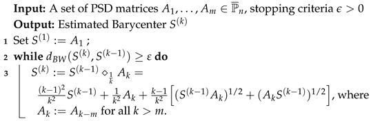
• Inductive Mean Algorithm (Algorithm 1) estimates the barycenter of $A_1,\dots ,A_m\in {\overline{P}}_n$ along the geodesic that connects two points on ${\overline{P}}_n$, as illustrated in Figure 1B with four data points as an example. The initial barycenter is set to be the first data point, $S^{\left(1\right)}:=A_1$, and then the barycenter is updated as the middle point along the geodesic that connects $S^{\left(1\right)}$ and $A_2$, i.e., $S^{\left(2\right)}:=S^{\left(1\right)}{\diamond }_{1/2}{A}_2$. In the iteration process, given $S^{(k-1)}$, the updated barycenter $S^{\left(k\right)}$ is the ${{\displaystyle \frac{1}{k}}}^{th}$ point along the geodesic connecting $S^{(k-1)}$ and $A_k$, with $A_k:=A_{k-m}$ for all $k>m$.

Algorithm 1: Inductive Mean Algorithm

By design, points in ${\left\{S^{\left(k\right)}\right\}}_{k\in \mathbb{N}}$ are confined within the compact region bound by the geodesics connecting $A_1,\dots ,A_m$, and the convergence point of ${\left\{S^{\left(k\right)}\right\}}_{k\in \mathbb{N}}$ is unique. Therefore, the Inductive Algorithm is valid for estimating the barycenter of PSD matrices. With the AI metric, the convergence of the algorithm to the corresponding Fréchet mean was proved in ([46] Theorem 5.2). With the BW metric, the computational process of the algorithm is straightforward and not sensitive to the quantity of matrices, as long as the maximal distance between two matrices in $A_1,\dots ,A_m$ is bounded. The convergence rate is uniform but relatively slow compared to the following two algorithms.

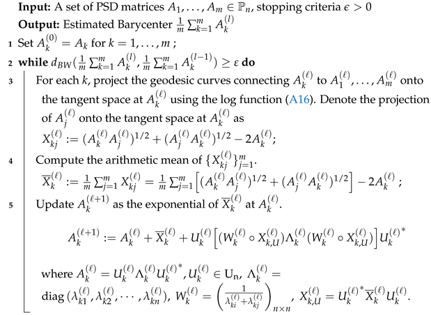
• Projection Mean Algorithm (Algorithm 2) accounts for the fact that the arithmetic center of the projections of $A_1,\dots ,A_m$ onto the tangent space at the barycenter C is exactly the projection of C (i.e., $0\in {\mathbb{H}}_n$). Inspired by this, the iteration starts with projecting the data points from ${\overline{P}}_n$ onto the tangent space at the arithmetic center of the original data. Then, the arithmetic mean of the tangent vectors is computed and projected back to ${\overline{P}}_n$ as the updated barycenter. The iteration stops when the distance between the estimated barycenter obtained in two consecutive iterations are less than the preset error tolerance $ϵ$. The details of the algorithm are summarized below.

Algorithm 2: Projection Mean Algorithm

The convergence of the Projection Mean Algorithm has been proved in the Wasserstein metric between probabilities ([47] Theorem 4.2), using a fixed point theorem approach. Here, we derive near order relations on the sequence $\{S^{\left(k\right)}\mid k\in \mathbb{N}\}$ and give a new proof for the convergence of the Projection Mean Algorithm for the BW metric.

It is well known that the Wasserstein barycenter $S:=\overline{A}(A_1,\dots ,A_m)$ is the unique matrix in ${\mathbb{P}}_n$ that satisfies the equation:

$$I={\displaystyle \frac{1}{m}}\sum _{j=1}^m[S^{-1}♯A_j].$$

(20)

We have the following property of the Projection Mean Algorithm.

Theorem 9.

For $A_1,\dots ,A_m\in {\overline{\mathbb{P}}}_n$ with at least one $A_j\in {\mathbb{P}}_n$, the sequence $\{S^{\left(k\right)}\mid k\in \mathbb{N}\}$ obtained from the Projection Mean Algorithm in the BW metric satisfies that

$${\left(S^{\left(k\right)}\right)}^{-1}♯S^{(k+1)}={\displaystyle \frac{1}{m}}\sum _{j=1}^m[{\left(S^{\left(k\right)}\right)}^{-1}♯A_j].$$

(21)

Equivalently,

$${\left(S^{\left(k\right)}{S}^{(k+1)}\right)}^{1/2}={\displaystyle \frac{1}{m}}\sum _{j=1}^m{\left(S^{\left(k\right)}{A}_j\right)}^{1/2}.$$

(22)

Proof. 

We have $S^{\left(k\right)}\in {\mathbb{P}}_n$ by induction. The Projection Mean Algorithm derives $S^{(k+1)}$ from $S^{\left(k\right)}$ through the process:

$${log}_{S^{\left(k\right)}}{S}^{(k+1)}={\displaystyle \frac{1}{m}}\sum _{j=1}^m{log}_{S^{\left(k\right)}}{A}_j.$$

Using formula (17), we have

$$\begin{array}{ccc}\hfill S^{\left(k\right)}[{\left(S^{\left(k\right)}\right)}^{-1}♯S^{(k+1)}]+[{\left(S^{\left(k\right)}\right)}^{-1}♯S^{(k+1)}]S^{\left(k\right)}& =& S^{\left(k\right)}\left[{\displaystyle \frac{1}{m}}\sum _{j=1}^m{\left(S^{\left(k\right)}\right)}^{-1}♯A_j\right]+\left[{\displaystyle \frac{1}{m}}\sum _{j=1}^m{\left(S^{\left(k\right)}\right)}^{-1}♯A_j\right]S^{\left(k\right)}.\hfill \end{array}$$

The matrix

$$C:=[{\left(S^{\left(k\right)}\right)}^{-1}♯S^{(k+1)}]-{\displaystyle \frac{1}{m}}\sum _{j=1}^m[{\left(S^{\left(k\right)}\right)}^{-1}♯A_j]$$

is Hermitian. The preceding equality shows that:

$$S^{\left(k\right)}C+C{S}^{\left(k\right)}=0.$$

So $S^{\left(k\right)}C$ is skew-Hermitian. Moreover, $S^{\left(k\right)}C$ is similar to the Hermitian matrix ${\left(S^{\left(k\right)}\right)}^{1/2}C{\left(S^{\left(k\right)}\right)}^{1/2}$, whose eigenvalues are all real. Hence, $S^{\left(k\right)}C=0$ and $C=0$. We obtain (21).

By [32], Proposition 4.1.9, $A♯B=A{\left(A^{-1}B\right)}^{1/2}$ for $A,B\in {\mathbb{P}}_n$. Apply it to (21) and we will get (22).    □

Theorem 10.

The sequence $\{S^{\left(k\right)}\mid k\in \mathbb{N}\}$ obtained from the Projection Mean Algorithm on $A_1,\dots ,A_m\in {\overline{P}}_n$ satisfies the Löwner order relations:

$${\displaystyle \frac{1}{m}}\sum _{j=1}^m{A}_j=S^{\left(0\right)}\ge S^{(k+1)},k\in \mathbb{N}.$$

(23)

Proof. 

For $n\times n$ Hermitian matrices $B_1,\dots ,B_m$ we have the Löwner order

$$\sum _{1\le i<j\le m}{(B_i-B_j)}^2\ge 0$$

(24)

which is equivalent to

$${\displaystyle \frac{1}{m}}\sum _{j=1}^m{B}_j^2\ge {\left({\displaystyle \frac{1}{m}}\sum _{j=1}^m{B}_j\right)}^2.$$

(25)

(21) can be expressed as

$${\left[{\left(S^{\left(k\right)}\right)}^{1/2}{S}^{(k+1)}{\left(S^{\left(k\right)}\right)}^{1/2}\right]}^{1/2}={\displaystyle \frac{1}{m}}\sum _{j=1}^m{\left[{\left(S^{\left(k\right)}\right)}^{1/2}{A}_j{\left(S^{\left(k\right)}\right)}^{1/2}\right]}^{1/2}.$$

(26)

So, for $k\in \mathbb{N}$ we have

$$\begin{array}{ccc}\hfill {\left(S^{\left(k\right)}\right)}^{1/2}\left({\displaystyle \frac{1}{m}}\sum _{j=1}^m{A}_j\right){\left(S^{\left(k\right)}\right)}^{1/2}& =& {\displaystyle \frac{1}{m}}\sum _{j=1}^m{\left(S^{\left(k\right)}\right)}^{1/2}{A}_j{\left(S^{\left(k\right)}\right)}^{1/2}\hfill \\ & \ge & {\left\{{\displaystyle \frac{1}{m}}\sum _{j=1}^m{\left[{\left(S^{\left(k\right)}\right)}^{1/2}{A}_j{\left(S^{\left(k\right)}\right)}^{1/2}\right]}^{1/2}\right\}}^2\hfill \\ & =& {\left(S^{\left(k\right)}\right)}^{1/2}{S}^{(k+1)}{\left(S^{\left(k\right)}\right)}^{1/2}.\hfill \end{array}$$

(27)

Therefore, ${\displaystyle \frac{1}{m}}{\sum }_{j=1}^m{A}_j\ge S^{(k+1)}$ for $k\in \mathbb{N}$.    □

• Cheap Mean Algorithm [48] (Algorithm 3) also utilizes the Log and Exp functions to project matrices between ${\overline{P}}_n$ and the tangent space. Different from the Projection Algorithm that only updates the estimated barycenter, the Cheap Mean Algorithm updates the estimated barycenter as well as the original matrices. Moreover, unlike the Projection Mean Algorithm that only spans the tangent space at the estimated barycenter $S^{\left(k\right)}$ in the iterations, the Cheap Mean Algorithm spans the tangent space at each data matrix. Specifically, for each original matrix $A_k$, which also serves as the initiation of $A_k^{\left(0\right)}$, all matrices are projected onto the tangent space spanned at $A_k$, then the arithmetic mean of the tangent vectors are projected back to ${\overline{P}}_n$ and serve as the update of $A_k$, denoted as $A_k^{\left(1\right)}$. Each data matrix is updated during the iteration process, and the iteration stops when the changes of the arithmetic mean of all updated matrices ($A_k^{(\ell )}$) is less than $ϵ$. The iterative process is outlined as follows:

Algorithm 3: Cheap Mean Algorithm

When $m=2$, the Cheap Mean Algorithm produces the true Fréchet Mean. However, when $m>2$, the Cheap Mean is only an approximation of the Fréchet Mean [48], compensated by the low computational cost of this algorithm [48,49]. Nevertheless, as shown in the following experimental results, the efficiency prowess of the Cheap Mean approach is only displayed when the number of matrices is small.

2.3. Classification with BW Barycenter

The barycenter serves not only as a statistical metric for measuring the central tendency of data, but is also extensively applied in the development of classifiers in various domains, including BCI research. Therefore, we construct a simple classifier known as the Minimum Distance to Riemannian Mean (MDRM) [50] as follows.

Suppose there are $m_k$ matrices belonging to the $k^{th}$ class, denoted as ($X_1^{\left(k\right)},\dots ,X_{m_k}^{\left(k\right)}$). Let ${\widehat{\mu }}_k$ denote the estimated barycenter of the $k^{\left(th\right)}$ class. The MDRM method compares the distance between a new matrix $X_{new}$ and the barycenter of each class, and assigns $X_{new}$ to the class whose barycenter exhibits the minimum distance.

$$k^{*}=\underset{k}{arg\; min}{d}_{\circ }(X_{new},{\widehat{\mu }}_k)$$

where $d_{\circ }(·,·)$ denote the chosen distance metric (e.g., AI and BW). It is crucial to note that the selection of metrics gives rise to distinct barycenters, and therefore, ${\widehat{\mu }}_k$ is contingent on the selected metric. Consequently, the classifier, when paired with distinct metrics, would demonstrate varying classification capabilities. With five real datasets, we aim to explore the efficacy of BW metric with this simple classifier and compare it with the widely used AI metric.

3. Simulation Results

Different metrics give rise to distinct barycenters. Although the true BW barycenter remains elusive, as there is no probability distribution defined on the manifold coupled with the BW metric yet, we can still conduct extensive simulations to thoroughly investigate the efficiency and robustness of the estimation of BW barycenter. In this section, we investigate both efficiency and robustness of the BW metric and barycenter and compare them with the AI metric and barycenter (1) via extensive simulations. Given that the AI metric is applicable only to positive definite matrices, we augment the randomly generated PSD matrices with a diagonal matrix ($O\left({10}^{-3}\right)\times I$) in order to ensure the positive definiteness of PSD matrices in our simulations.

Table 1. Simulation Parameter Settings.

Simulation Parameter	Values
n: Dimension of Matrices	$[5,10,20,30,50,100]$
m: Number of Matrices	$[5,10,20,30,50,100]$
p: Proportion of zero eigenvalues	$[0.1,0.2,0.4,0.6,0.8]$

provides a summary of the parameter settings employed in the following simulations.

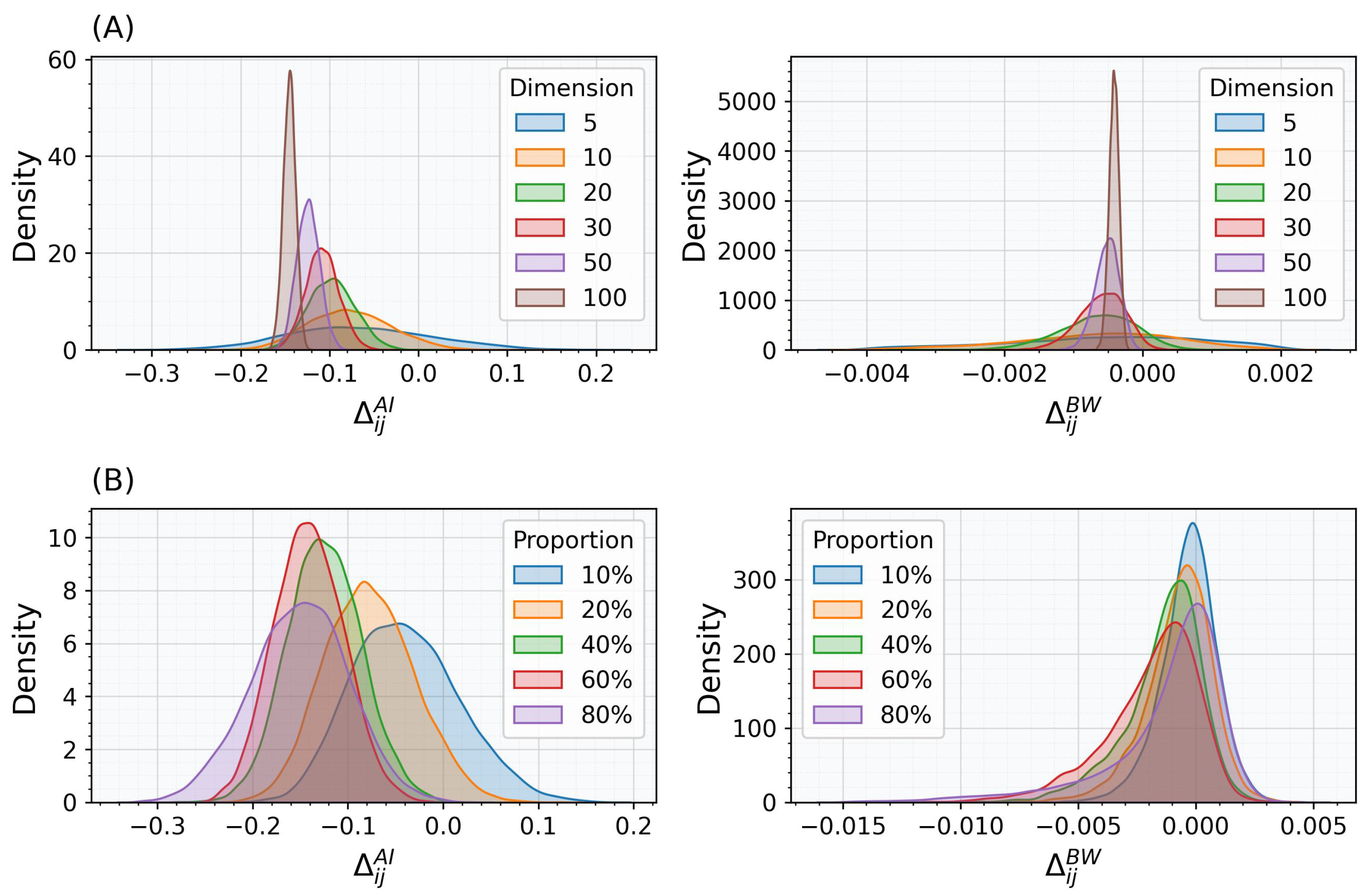
3.1. Robustness of BW Distance

When matrices are affected by slight perturbations, a robust distance measure is expected to remain unaffected, i.e., small changes in distance. In this simulation, we quantify the robustness of a distance measure as the alteration in distance values when matrices are affected by slight perturbations. Our goal is to assess the robustness of BW distance and investigate the factors that affect its robustness.

We begin by randomly generating 100 pairs of PSD matrices, denoted as $(A_i,B_i)$, $i=1,\dots ,100$, where dimension n is set to 10 and p is set to 0.2. For each pair $(A_i,B_i)$, we randomly generate 100 pairs of Hermitian perturbation matrices, denoted as $(E_{ij}^A,E_{ij}^B)$, $j=1,\dots ,100$. These perturbation matrices have spectral norms scaled to match the smallest eigenvalues of $(A_i,B_i)$, which is $O\left({10}^{-3}\right)$. The contaminated matrices $({\tilde{A}}_{ij},{\tilde{B}}_{ij})$ are then obtained by adding the perturbation matrices to $(A_i,B_i)$, resulting in ${\tilde{A}}_{ij}=A_i+E_{ij}^A$, ${\tilde{B}}_{ij}=B_i+E_{ij}^B$. The robustness of the distance measures is assessed by quantifying the difference in distances between the two matrices with and without perturbation. As AI and BW distance are different, we normalize the differences by the respective distance measure between the unperturbed matrices as follows:

$${\Delta }_{ij}^{AI}={\displaystyle \frac{d_{AI}(A_i,B_i)-d_{AI}({\tilde{A}}_{ij},{\tilde{B}}_{ij})}{d_{AI}(A_i,B_i)}},{\Delta }_{ij}^{BW}={\displaystyle \frac{d_{BW}(A_i,B_i)-d_{BW}({\tilde{A}}_{ij},{\tilde{B}}_{ij})}{d_{BW}(A_i,B_i)}}.$$

Figure 2 presents the empirical distributions of ${\Delta }_{ij}^{AI}$ and ${\Delta }_{ij}^{BW}$ with varying n in (A) and varying p in (B). Overall, ${\Delta }^{BW}$ consistently exhibits significantly smaller values compared to ${\Delta }^{AI}$, indicating the superior robustness of BW distance in the presence of perturbations. Moreover, both BW and AI distances are influenced by the matrix dimension (all p-values $<0.01$ for Kruskal–Wallis and Dunn tests), with higher dimensions resulting in reduced robustness. However, p has less impact on the robustness of both distances (significant Kruskal–Wallis test, but not all p-values are significant for Dunn tests at $0.01$ significance level). Additionally, BW distance demands considerably less computational time than AI distance, as evident from the comparison of Equations (1) and (4).

3.2. Robustness of BW Barycenter for Two Matrices

The true BW barycenter of two matrices is the midpoint along the geodesic. There is no necessity to employ an algorithm for barycenter estimation in this case. Hence, we evaluate the robustness of the BW barycenter for a pair of matrices independently. The robustness refers to whether the barycenter would be affected when the two matrices are contaminated by small perturbations. With this simulation, we aim to assess the robustness of the BW barycenter and investigate the factors that affect its robustness.

Following the same data simulation process outlined previously, we randomly generate 100 pairs of unperturbed matrices $(A_i,B_i),i=1,\dots ,100$. For each pair $(A_i,B_i)$, 100 perturbed matrices $({\tilde{A}}_{ij},{\tilde{B}}_{ij}),j=1,\dots ,100$ are generated. Then, the BW and AI barycenters for unperturbed and perturbed matrices are computed:

$$M_i^{AI}=A_i♯B_i,M_i^{BW}=A_i\diamond B_i$$

$${\tilde{M}}_{ij}^{AI}={\tilde{A}}_{ij}♯{\tilde{B}}_{ij},{\tilde{M}}_{ij}^{BW}={\tilde{A}}_{ij}\diamond {\tilde{B}}_{ij}$$

The robustness of the barycenter is quantified as the Frobenius distance between the barycenters of matrices with and without perturbations, denoted as $d_F(M_i^{\circ },{\tilde{M}}_{ij}^{\circ })$ for AI and BW measures, respectively. A smaller distance $d_F(M_i^{\circ },{\tilde{M}}_{ij}^{\circ })$ indicates greater robustness of the barycenter. Figure 3 presents the distribution of $\left\{d_F(M_i^{\circ },{\tilde{M}}_{ij}^{\circ })\right\},j=1,\dots ,100$ for three representative pairs of matrices. Case 1 represents the most prevalent scenario ($73\%$) where $d_F(M_i^{BW},{\tilde{M}}_{ij}^{BW})$ is generally smaller than $d_F(M_i^{AI},{\tilde{M}}_{ij}^{AI})$. Case 2 shows another common scenario ($25\%$) when $d_F(M_i^{BW},{\tilde{M}}_{ij}^{BW})$ is significantly smaller than $d_F(M_i^{AI},{\tilde{M}}_{ij}^{AI})$. Both case 1 and 2 signify instances where the BW barycenter exhibits greater robustness than the AI barycenter. In contrast, Case 3, which is the least common scenario ($2\%$), showcases situations where the AI barycenter displays superior robustness to the BW barycenter, albeit with a noteworthy degree of overlap between the two distributions.

For each pair of matrices, the average of $\left\{d_F(M_i^{\circ },{\tilde{M}}_{ij}^{\circ })\right\}$, denoted as $\overline{d_F(M_i^{\circ },{\tilde{M}}_{ij}^{\circ })}$, are calculated for AI and BW, respectively, to represent the average deviation of the barycenter when matrices are affected by perturbations. To compare which barycenter is less affected by the perturbation, i.e., the one having smaller $\overline{d_F(M_i^{\circ },{\tilde{M}}_{ij}^{\circ })}$, we record the relative difference ${\delta }_i$ as follows:

$$\overline{d_F(M_i^{\circ },{\tilde{M}}_{ij}^{\circ })}={\displaystyle \frac{1}{100}}\sum _{j=1}^{100}{d}_F(M_i^{\circ },{\tilde{M}}_{ij}^{\circ }),{\delta }_i={\displaystyle \frac{\overline{d_F(M_i^{AI},{\tilde{M}}_{ij}^{AI})}-\overline{d_F(M_i^{BW},{\tilde{M}}_{ij}^{BW})}}{\overline{d_F(M_i^{BW},{\tilde{M}}_{ij}^{BW})}}}.$$

A positive ${\delta }_i$ signifies that the BW barycenter exhibits greater robustness compared to AI. Figure 4A,B presents the distribution of $\left\{\delta \right\}$ with varying n and p, respectively. The line plot in the top right corner describes the median of each $\left\{\delta \right\}$ distribution. Overall, a substantial portion of $\delta$ fall on the positive side, irrespective of n and p, while occurrences of negative $\delta$ are rare. This pattern indicates that the BW barycenter tends to be more robust than the AI barycenter.

With an increase in the matrix dimension n, the distribution of ${\delta }_i$ becomes more tightly clustered around 0, accompanied by a consistent decrease in the median. In simpler terms, the advantage in robustness of the BW barycenter over AI is more pronounced for lower-dimensional matrices (significant Kruskal–Wallis test and majority pairwise comparisons of Dunn test are significant at significant level $0.05$). Unlike n, the distribution of $\delta$ exhibits similar shapes and comparable medians across varying p (not significant Kruskal–Wallis test). Consequently, it appears that p exerts minimal influence on the discrepancies in robustness between BW and AI barycenters.

3.3. Properties of BW Barycenter for More than Two Matrices

Now we consider a collection of PSD matrices $A_1,\dots ,A_m,m>2$ and estimate their barycenter using the proposed algorithms. Our goal is to evaluate the efficiency, accuracy, and robustness of the BW barycenter estimation.

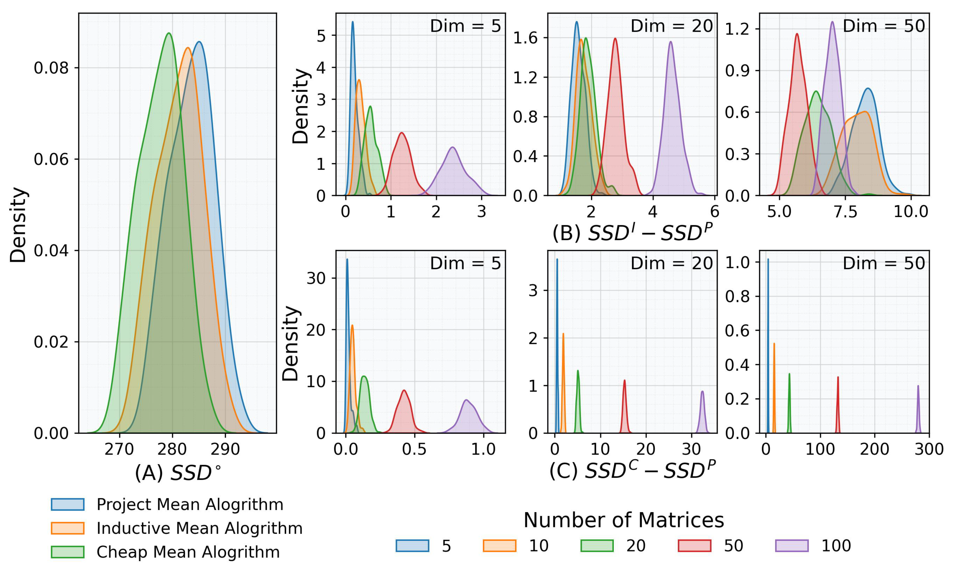
3.3.1. Efficiency of Barycenter Estimation with BW Distance

The three algorithms are applied to multiple sets of randomly generated PSD matrices to estimate both the BW and AI barycenters. Figure 5 presents the average runtime (in seconds) on a logarithmic scale for various numbers and dimensions of matrices. For each combination of dimension of matrices n and number of matrices m, 100 sets of matrices are generated.

Both the Projection and Cheap Mean Algorithms require more time to execute as n or m increases, whereas the Inductive Algorithms is primarily only affected by n. The BW Projection Algorithm (abbreviation of Projection Algorithm with BW distance) proves to be the most efficient regardless of n or m, followed by the AI Projection Algorithm in second place. The gap between the two diminishes as n increases. It is also worth emphasizing that the AI Projection Algorithm could experience convergence difficulties, especially when n substantially surpasses m [49]. For evidence, see Section 4.

3.3.2. Accuracy of Barycenter Estimation with BW Distance

The barycenter of a set of matrices, although unknown, is defined as the point that minimizes the sum of squared BW distances from each matrix to itself. This makes the sum of squared distances (SSD) a suitable metric for measuring the accuracy of the barycenter estimation, where a smaller SSD indicates a more accurate estimation of the barycenter.

A set of PSD matrices are randomly generated, with p being 0.2 and varying m and n. Three algorithms are employed to estimate the barycenters using the same stopping criteria $\epsilon ={10}^{-3}$. Denote the barycenter estimated via the Inductive, Projection, and Cheap Mean Algorithm as $M^I$, $M^P$, and $M^C$, respectively. For each barycenter $M^{\circ }$, the corresponding $SS{D}^{\circ }$ is calculated as $SS{D}^{\circ }={\sum }_{i=1}^m{d}_{BW}^2(A_i,M^{\circ })$. Figure 6A shows the distribution of three $SS{D}^{\circ }$ across 100 iterations with n being 10 and m being 100. $SS{D}^P$ is significantly smaller than the other two. For easy comparison, we present the difference between $SS{D}^I$ and $SS{D}^P$ in Figure 6B and difference between $SS{D}^C$ and $SS{D}^P$ in Figure 6C.

Overall, both $SS{D}^I-SS{D}^P$ and $SS{D}^C-SS{D}^P$ are positive, indicating that the Projection Mean Algorithm consistently proves to be the most accurate, regardless of n and m. $SS{D}^C-SS{D}^P$ generally exhibits a larger scale than $SS{D}^I-SS{D}^P$, implying that the Inductive Mean Algorithm tends to outperform the Cheap Mean Algorithm, except for low-dimensional matrices $n=5$. Additionally, the Cheap Mean Algorithm exhibits reduced accuracy with increasing number and dimension of matrices.

3.3.3. Robustness of Barycenter Estimation with BW Distance

The robustness of barycenter estimation refers to how the estimated barycenter is affected by perturbations introduced to the matrices. To assess this, we use the Frobenius distance between the two barycenters estimated with and without perturbations as the evaluation metric, with the assumption that a smaller distance indicates a more robust barycenter. Given that the Projection Algorithm is the most precise and efficient, it is employed for estimating the barycenters in this simulation for both the AI and BW metric. In the cases where AI Projection encounters convergence issues, we resort to AI Inductive for barycenter estimation.

In each iteration i ($i=1,\dots ,100$), a set of PSD matrices $\{A_i^1,\dots ,A_i^m\}$ is randomly generated, and the contaminated matrices $\{{\tilde{A}}_{ij}^1,\dots ,{\tilde{A}}_{ij}^m,j=1,\dots ,100\}$ are derived by adding randomly generated Hermitian perturbation matrices $E_{ij}^k$ to $A_i^k$. Let $M_i^{BW}$ and $M_i^{AI}$ denote the estimated barycenters of unperturbed matrices $\{A_i^1,\dots ,A_i^m\}$, and ${\tilde{M}}_{ij}^{BW}$ and ${\tilde{M}}_{ij}^{AI}$ represent the barycenters of perturbed matrices $\{{\tilde{A}}_{ij}^1,\dots ,{\tilde{A}}_{ij}^m\}$. The robustness of barycenter is then assessed via $d_F(M_i^{\circ },{\tilde{M}}_{ij}^{\circ })$. Figure 7A presents the distribution of $\left\{d_F(M_i^{BW},{\tilde{M}}_{ij}^{BW})\right\}$ and Figure 7B presents the distribution of $\{d_F(M_i^{AI},{\tilde{M}}_{ij}^{AI})-d_F(M_i^{BW},{\tilde{M}}_{ij}^{BW})\}$. It is observed that as n or m increases, BW barycenters exhibit significantly greater robustness than AI barycenters (confirmed by a significant Kruskal–Wallis test and pairwise Wilcoxon Rank Sum test).

4. Real Data Results

In addition to simulations, we also investigate the effectiveness of employing BW distance and BW barycenter in real-world applications. One scalp EEG data collected in a lab and four publicly accessible BCI datasets are utilized to evaluate the improvement in classification performance achieved through the implementation of BW distance.

Two datasets from BCI competition III [51,52,53] and two from BCI competition IV [54,55,56] are utilized in order to ensure a comprehensive representation of scenarios commonly encountered in EEG-based BCI applications. In BCI III, dataset IIIa comprises 60-channel EEG recordings from three subjects who performed motor imagery tasks involving four classes (left hand, right hand, foot, and tongue). Dataset IVa consists of 118-channel EEG recordings from five subjects engaged in two motor imagery tasks (right hand and foot). In BCI IV, dataset IIa includes 22-channel EEG recordings from nine subjects performing four motor imagery tasks (left hand, right hand, feet, and tongue), while dataset IIb contains 3-channel EEG recordings from nine subjects engaged in two tasks (left hand and right hand). For the sake of comparability across all datasets, the two datasets with four classes were narrowed down to two classes, i.e., right hand and left hand, so that the classification on all datasets are framed as a binary task. Besides BCI data, one scalp EEG data collected from human spatial cognition laboratory at the University of Arizona is also incorporated. In total, 16 participants were recruited to perform predesigned tasks. Written informed consent was obtained from participants. The study was approved by the Institutional Review Board at the University of Arizona and is conducted in accordance with relevant guidelines and regulations. The EEG data is a 64-channel scalp EEG with binary labels. Further information regarding the experimental design can be found in [2,57]. Details regarding the five datasets are summarized in

Table 2. The configurations and classifications of BCI datasets.

	BCI III		BCI IV		Lab Data
	Dataset IIIa	Dataset IVa	Dataset IIa	Dataset IIb
Number of subjects	3	5	9	9	16
Number of channels	60	118	22	3	64
Trials per class	30/45	28–224	72	60/70/80	9–17
Sampling rate	250 Hz	1000 Hz	250 Hz	250 Hz	500 Hz
Filter Band	8–30 Hz	8–30 Hz	8–30 Hz	8–30 Hz	1–30 Hz
Classification Performance
Accuracy (BW)	0.68	0.72	0.70	0.66	0.99
Accuracy (BW with LWF)	0.59	0.65	0.76	0.58	0.89
Accuracy (AI)	0.58	0.62	0.66	0.66	0.88
Accuracy (AI with LWF)	0.63	0.71	0.75	0.58	0.90

. In general, the matrix dimensions across these five datasets range from 3 to 118, and the number of matrices varies from 10 to 200. This provides a broad and inclusive representation of the cases encountered in EEG-based BCI data analysis.

Let $S_{n\times T}$ represent the BCI (or EEG) data, with n denoting the number of electrode channels and T indicating the duration of each trial. Following the preprocessing procedures outlined in the previous works [5,6,58,59,60], the raw BCI undergo bandpass filtration within the 8–30 Hz range utilizing a fifth-order Butterworth filter. Similarly, the lab EEG data undergoes a bandpass filter of 1–30 Hz and independent component analysis [57]. Subsequently, the covariance matrix of the filtered signals during each trial is computed, denoted as $X_{n\times n}$. Then, a MDRM classifier is trained to directly classify the matrix $X_{n\mathrm{x}n}$ into one of the classes. Using six-fold cross validation repeated 10 times, Table 2 presents the average classification accuracy for the five datasets. The barycenters in the MDRM classifiers are estimated using the Projection Algorithm with the AI and BW metrics, respectively. Since covariance regularization is widely used in EEG preprocessing, we apply the Lediot–Wolf shrinkage method [61] (LWF) to explore the effect of regularization coupled with the two metrics, respectively.

Overall, it is evident that classifiers with BW barycenter yields higher accuracy when LWF is not applied. For BCI III IIIa, BCI III Iva, and the lab data, applying LWF decreases the accuracy of BW MDRM (abbreviation of MDRM classifier with BW barycenter) and increases the accuracy of AI MDRM. However, the increased accuracy of AI MDRM with LWF still falls short compared to BW MDRM without LWF. This, coupled with the extra cost of introducing LWF as an additional preprocessing step, suggests that preserving and modeling the positive semidefiniteness of matrices could be a superior option to regularization. On the other hand, AI and BW MDRM both produce decreased accuracy for BCI IV IIb, while both producing increased accuracy for BCI IV IIa. Although these two cases experience completely opposite changes, the performance of AI MDRM did not exceed its BW counterpart.

Moreover, using the AI metric in MDRM encountered convergence difficulties that using the BW metric did not encounter in our real data experiment. To measure the convergence process of the Projection Algorithms with the AI and BW metric, we recorded the sum of squared distances (SSD) after each iteration. The ’foot’ class of three subjects (av, aw, and ay) from the BCI III IVa dataset that share the same dimension of matrix ($n=118$) but have different number of matrices ($m=84$ for av, 56 for aw, and 28 for ay) were selected as representative cases for demonstration. The change in SSD is shown in Figure 8. In addition to the fact that the BW metric yielded significantly lower SSD than the AI metric, the numerically significant oscillatory behavior exhibited by using the AI metric suggests that the mean might be bouncing around in a neighborhood, while fast convergence is achieved by using the BW metric on the same data.

5. Conclusions

In this paper, we establish the mathematical framework for the BW distance by delving into its properties and the retraction maps of ${\overline{\mathbb{P}}}_n$. Given a set of PSD matrices, we propose three algorithms to estimate their barycenter, which characterize the central tendency of a set of matrices and is widely used in the construction of classifiers. Extensive simulation experiments reveal that BW distance and barycenter exhibit superior efficiency and robustness compared to AI distance, especially when dealing with high-dimensional matrices which are frequently encountered in high-dimensional data analysis. Moreover, validation with five real datasets further confirms the superiority of BW distance and BW barycenter. BW distance demonstrates higher classification accuracy and substantially reduced computational cost, especially for high-dimensional matrices. Therefore, when analyzing high-dimensional data, we highly recommend employing BW distance along with the Projection Mean Algorithm for the barycenter estimation. This approach eliminates the need for matrix regularization, substantially reduces computational time, and can achieve comparable or even superior classification performance compared to the AI metric. While we validate the proposed method using BCI data, it is adaptable to various other fields, including computer vision, remote sensing, and biomedical imaging.

References

1. Schirrmeister, R.T.; Springenberg, J.T.; Fiederer, L.D.J.; Glasstetter, M.; Eggensperger, K.; Tangermann, M.; Hutter, F.; Burgard, W.; Ball, T. Deep learning with convolutional neural networks for EEG decoding and visualization. Hum. Brain Mapp. 2017, 38, 5391–5420. [Google Scholar] [CrossRef]
2. Zheng, J.; Liang, M.; Sinha, S.; Ge, L.; Yu, W.; Ekstrom, A.; Hsieh, F. Time-frequency analysis of scalp EEG with Hilbert-Huang transform and deep learning. IEEE J. Biomed. Health Inform. 2021, 26, 1549–1559. [Google Scholar] [CrossRef] [PubMed]
3. Qiu, A.; Lee, A.; Tan, M.; Chung, M.K. Manifold learning on brain functional networks in aging. Med. Image Anal. 2015, 20, 52–60. [Google Scholar] [CrossRef] [PubMed]
4. Varoquaux, G.; Baronnet, F.; Kleinschmidt, A.; Fillard, P.; Thirion, B. Detection of brain functional-connectivity difference in post-stroke patients using group-level covariance modeling. In Proceedings of the Medical Image Computing and Computer-Assisted Intervention–MICCAI 2010: 13th International Conference, Beijing, China, 20–24 September 2010; Proceedings, Part I 13. Springer: Berlin/Heidelberg, Germany, 2010; pp. 200–208. [Google Scholar]
5. Barachant, A.; Bonnet, S.; Congedo, M.; Jutten, C. Riemannian Geometry Applied to BCI Classification. In Proceedings of the Latent Variable Analysis and Signal Separation, St. Malo, France, 27–30 September 2010; Vigneron, V., Zarzoso, V., Moreau, E., Gribonval, R., Vincent, E., Eds.; Springer: Berlin/Heidelberg, Germany, 2010; pp. 629–636. [Google Scholar]
6. Barachant, A.; Bonnet, S.; Congedo, M.; Jutten, C. Classification of Covariance Matrices Using a Riemannian-Based Kernel for BCI Applications. Neurocomput. 2013, 112, 172–178. [Google Scholar] [CrossRef]
7. Miah, A.S.M.; Islam, M.R.; Molla, M.K.I. EEG classification for MI-BCI using CSP with averaging covariance matrices: An experimental study. In Proceedings of the 2019 International Conference on Computer, Communication, Chemical, Materials and Electronic Engineering (IC4ME2), Rajshahi, Bangladesh, 1–12 July 2019; IEEE: Piscataway, NJ, USA, 2019; pp. 1–5. [Google Scholar]
8. Chen, K.X.; Ren, J.Y.; Wu, X.J.; Kittler, J. Covariance descriptors on a Gaussian manifold and their application to image set classification. Pattern Recognit. 2020, 107, 107463. [Google Scholar] [CrossRef]
9. Porikli, F.; Tuzel, O.; Meer, P. Covariance tracking using model update based on lie algebra. In Proceedings of the 2006 IEEE Computer Society Conference on Computer Vision and Pattern Recognition (CVPR’06), New York, NY, USA, 17–22 June 2006; IEEE: Piscataway, NJ, USA, 2006; Volume 1, pp. 728–735. [Google Scholar]
10. Sivalingam, R.; Boley, D.; Morellas, V.; Papanikolopoulos, N. Tensor sparse coding for region covariances. In Proceedings of the Computer Vision–ECCV 2010: 11th European Conference on Computer Vision, Heraklion, Crete, Greece, 5–11 September 2010; Proceedings, Part IV 11. Springer: Berlin/Heidelberg, Germany, 2010; pp. 722–735. [Google Scholar]
11. Jagarlamudi, J.; Udupa, R.; Daumé III, H.; Bhole, A. Improving bilingual projections via sparse covariance matrices. In Proceedings of the 2011 Conference on Empirical Methods in Natural Language Processing, Edinburgh, UK, 27–29 July 2011; pp. 930–940. [Google Scholar]
12. Zhang, W.; Fung, P. Discriminatively trained sparse inverse covariance matrices for speech recognition. IEEE/ACM Trans. Audio Speech Lang. Process. 2014, 22, 873–882. [Google Scholar] [CrossRef]
13. Cui, Z.; Li, W.; Xu, D.; Shan, S.; Chen, X.; Li, X. Flowing on Riemannian Manifold: Domain Adaptation by Shifting Covariance. IEEE Trans. Cybern. 2014, 44, 2264–2273. [Google Scholar] [CrossRef]
14. Zhang, Z.; Wang, M.; Huang, Y.; Nehorai, A. Aligning infinite-dimensional covariance matrices in reproducing kernel hilbert spaces for domain adaptation. In Proceedings of the IEEE Conference on Computer Vision and Pattern Recognition, Salt Lake City, UT, USA, 18–23 June 2018; pp. 3437–3445. [Google Scholar]
15. He, N.; Fang, L.; Li, S.; Plaza, A.; Plaza, J. Remote sensing scene classification using multilayer stacked covariance pooling. IEEE Trans. Geosci. Remote Sens. 2018, 56, 6899–6910. [Google Scholar] [CrossRef]
16. Eklundh, L.; Singh, A. A comparative analysis of standardised and unstandardised principal components analysis in remote sensing. Int. J. Remote Sens. 1993, 14, 1359–1370. [Google Scholar] [CrossRef]
17. Yang, D.; Gu, C.; Dong, Z.; Jirutitijaroen, P.; Chen, N.; Walsh, W.M. Solar irradiance forecasting using spatial-temporal covariance structures and time-forward kriging. Renew. Energy 2013, 60, 235–245. [Google Scholar] [CrossRef]
18. Meyer, K. Factor-analytic models for genotype× environment type problems and structured covariance matrices. Genet. Sel. Evol. 2009, 41, 21. [Google Scholar] [CrossRef]
19. Huang, Z.; Wang, R.; Shan, S.; Chen, X. Face recognition on large-scale video in the wild with hybrid Euclidean-and-Riemannian metric learning. Pattern Recognit. 2015, 48, 3113–3124. [Google Scholar] [CrossRef]
20. Arsigny, V.; Fillard, P.; Pennec, X.; Ayache, N. Geometric means in a novel vector space structure on symmetric positive-definite matrices. SIAM J. Matrix Anal. Appl. 2007, 29, 328–347. [Google Scholar] [CrossRef]
21. Jayasumana, S.; Hartley, R.; Salzmann, M.; Li, H.; Harandi, M. Kernel methods on the Riemannian manifold of symmetric positive definite matrices. In Proceedings of the IEEE Conference on Computer Vision and Pattern Recognition, Portland, OR, USA, 23–28 June 2013; pp. 73–80. [Google Scholar]
22. Huang, Z.; Wang, R.; Shan, S.; Li, X.; Chen, X. Log-euclidean metric learning on symmetric positive definite manifold with application to image set classification. In Proceedings of the International Conference on Machine Learning, PMLR, Lille, France, 6–11 July 2015; pp. 720–729. [Google Scholar]
23. Lin, Z. Riemannian geometry of symmetric positive definite matrices via Cholesky decomposition. SIAM J. Matrix Anal. Appl. 2019, 40, 1353–1370. [Google Scholar] [CrossRef]
24. Pennec, X. Manifold-valued image processing with SPD matrices. In Riemannian Geometric Statistics in Medical Image Analysis; Elsevier: Amsterdam, The Netherlands, 2020; pp. 75–134. [Google Scholar]
25. Ledoit, O.; Wolf, M. A well-conditioned estimator for large-dimensional covariance matrices. J. Multivar. Anal. 2004, 88, 365–411. [Google Scholar] [CrossRef]
26. Kotz, S.; Johnson, N.L. (Eds.) Breakthroughs in Statistics: Methodology and Distribution; Springer Series in Statistics; Perspectives in Statistics; Springer: New York, NY, USA, 1992; Volume II, pp. xxii+600. [Google Scholar]
27. Villani, C. Topics in Optimal Transportation; Graduate Studies in Mathematics; American Mathematical Society: Providence, RI, USA, 2003; Volume 58, pp. xvi+370. [Google Scholar] [CrossRef]
28. Villani, C. Optimal Transport: Old and New; Grundlehren der Mathematischen Wissenschaften [Fundamental Principles of Mathematical Sciences]; Springer: Berlin/Heidelberg, Germany, 2009; Volume 338, pp. xxii+973. [Google Scholar] [CrossRef]
29. Hayashi, M. Quantum Information Theory: Mathematical Foundation, 2nd ed.; Graduate Texts in Physics; Springer: Berlin/Heidelberg, Germany, 2017; pp. xli+636. [Google Scholar] [CrossRef]
30. Bengtsson, I.; Życzkowski, K. Geometry of Quantum States: An Introduction to Quantum Entanglement, 2nd ed.; Cambridge University Press: Cambridge, UK, 2017; pp. xv+619. [Google Scholar] [CrossRef]
31. Oostrum, J.v. Bures-Wasserstein geometry for positive-definite Hermitian matrices and their trace-one subset. Inf. Geom. 2022, 5, 405–425. [Google Scholar] [CrossRef]
32. Bhatia, R. Positive Definite Matrices; Princeton Series in Applied Mathematics; Princeton University Press: Princeton, NJ, USA, 2007; pp. x+254. [Google Scholar]
33. Bhatia, R.; Jain, T.; Lim, Y. On the Bures—Wasserstein distance between positive definite matrices. Expo. Math. 2019, 37, 165–191. [Google Scholar] [CrossRef]
34. Bhatia, R.; Jain, T.; Lim, Y. Inequalities for the Wasserstein mean of positive definite matrices. Linear Algebra Its Appl. 2019, 576, 108–123. [Google Scholar] [CrossRef]
35. Thanwerdas, Y.; Pennec, X. O(n)-invariant Riemannian metrics on SPD matrices. Linear Algebra Its Appl. 2023, 661, 163–201. [Google Scholar] [CrossRef]
36. Hwang, J.; Kim, S. Two-variable Wasserstein means of positive definite operators. Mediterr. J. Math. 2022, 19, 110. [Google Scholar] [CrossRef]
37. Thanwerdas, Y. Riemannian and Stratified Geometries of Covariance and Correlation Matrices. Ph.D. Thesis, Université Côte d’Azur, Nice, France, 2022. [Google Scholar]
38. Kim, S.; Lee, H. Inequalities of the Wasserstein mean with other matrix means. Ann. Funct. Anal. 2020, 11, 194–207. [Google Scholar] [CrossRef]
39. Hwang, J.; Kim, S. Bounds for the Wasserstein mean with applications to the Lie-Trotter mean. J. Math. Anal. Appl. 2019, 475, 1744–1753. [Google Scholar] [CrossRef]
40. Massart, E.; Absil, P.A. Quotient geometry with simple geodesics for the manifold of fixed-rank positive-semidefinite matrices. SIAM J. Matrix Anal. Appl. 2020, 41, 171–198. [Google Scholar] [CrossRef]
41. Malagò, L.; Montrucchio, L.; Pistone, G. Wasserstein Riemannian geometry of Gaussian densities. Inf. Geom. 2018, 1, 137–179. [Google Scholar] [CrossRef]
42. Kubo, F.; Ando, T. Means of positive linear operators. Math. Ann. 1980, 246, 205–224. [Google Scholar] [CrossRef]
43. Lee, H.; Lim, Y. Metric and spectral geometric means on symmetric cones. Kyungpook Math. J. 2007, 47, 133–150. [Google Scholar]
44. Gan, L.; Huang, H. Order relations of the Wasserstein mean and the spectral geometric mean. Electron. J. Linear Algebra 2024, 40, 491–505. [Google Scholar] [CrossRef]
45. Yger, F.; Berar, M.; Lotte, F. Riemannian Approaches in Brain-Computer Interfaces: A Review. IEEE Trans. Neural Syst. Rehabil. Eng. 2017, 25, 1753–1762. [Google Scholar] [CrossRef]
46. Lim, Y.; Pálfia, M. Weighted inductive means. Linear Algebra Appl. 2014, 453, 59–83. [Google Scholar] [CrossRef]
47. Álvarez Esteban, P.C.; del Barrio, E.; Cuesta-Albertos, J.; Matrán, C. A fixed-point approach to barycenters in Wasserstein space. J. Math. Anal. Appl. 2016, 441, 744–762. [Google Scholar] [CrossRef]
48. Bini, D.A.; Iannazzo, B. A note on computing matrix geometric means. Adv. Comput. Math. 2011, 35, 175–192. [Google Scholar] [CrossRef]
49. Jeuris, B.; Vandebril, R.; Vandereycken, B. A survey and comparison of contemporary algorithms for computing the matrix geometric mean. Electron. Trans. Numer. Anal. 2012, 39, 379–402. [Google Scholar]
50. Barachant, A.; Bonnet, S.; Congedo, M.; Jutten, C. Multiclass Brain–Computer Interface Classification by Riemannian Geometry. IEEE Trans. Biomed. Eng. 2012, 59, 920–928. [Google Scholar] [CrossRef]
51. Blankertz, B.; Muller, K.R.; Krusienski, D.J.; Schalk, G.; Wolpaw, J.R.; Schlogl, A.; Pfurtscheller, G.; Millan, J.R.; Schroder, M.; Birbaumer, N. The BCI competition III: Validating alternative approaches to actual BCI problems. IEEE Trans. Neural Syst. Rehabil. Eng. 2006, 14, 153–159. [Google Scholar] [CrossRef]
52. Schlögl, A. GDF-A general dataformat for biosignals. arXiv 2006, arXiv:cs/0608052. [Google Scholar]
53. Dornhege, G.; Blankertz, B.; Curio, G.; Muller, K.R. Boosting bit rates in noninvasive EEG single-trial classifications by feature combination and multiclass paradigms. IEEE Trans. Biomed. Eng. 2004, 51, 993–1002. [Google Scholar] [CrossRef] [PubMed]
54. Tangermann, M.; Müller, K.R.; Aertsen, A.; Birbaumer, N.; Braun, C.; Brunner, C.; Leeb, R.; Mehring, C.; Miller, K.J.; Mueller-Putz, G.; et al. Review of the BCI competition IV. Front. Neurosci. 2012, 6, 55. [Google Scholar]
55. Brunner, C.; Leeb, R.; Müller-Putz, G.; Schlögl, A.; Pfurtscheller, G. BCI Competition 2008–Graz Data Set A; IEEE DataPort: Piscataway, NJ, USA, 2008; Volume 16, pp. 1–6. [Google Scholar] [CrossRef]
56. Leeb, R.; Brunner, C.; Müller-Putz, G.; Schlögl, A.; Pfurtscheller, G. BCI Competition 2008–Graz Data Set B; Graz University of Technology: Graz, Austria, 2008; Volume 16, pp. 1–6. [Google Scholar]
57. Liang, M.; Starrett, M.J.; Ekstrom, A.D. Dissociation of frontal-midline delta-theta and posterior alpha oscillations: A mobile EEG study. Psychophysiology 2018, 55, e13090. [Google Scholar] [CrossRef]
58. Lotte, F.; Guan, C. Regularizing common spatial patterns to improve BCI designs: Unified theory and new algorithms. IEEE Trans. Biomed. Eng. 2010, 58, 355–362. [Google Scholar] [CrossRef]
59. Barachant, A.; Bonnet, S.; Congedo, M.; Jutten, C. BCI Signal Classification using a Riemannian-based kernel. In Proceedings of the 20th European Symposium on Artificial Neural Networks, Computational Intelligence and Machine Learning (ESANN 2012), Bruges, Belgium, 25–27 April 2012; pp. 97–102. [Google Scholar]
60. Congedo, M.; Barachant, A.; Bhatia, R. Riemannian geometry for EEG-based brain–computer interfaces; a primer and a review. Brain-Comput. Interfaces 2017, 4, 155–174. [Google Scholar] [CrossRef]
61. Ledoit, O.; Wolf, M. Honey, I shrunk the sample covariance matrix. J. Portf. Manag. 2004, 30, 110–119. [Google Scholar] [CrossRef]
Figure 1. (A) Manifold and its tangent space at point A P ¯ n . (B) Illustration of the Inductive Algorithm.
Mathematics 13 02157 g001
Figure 2. Empirical distributions of Δ i j A I and Δ i j B W under different dimension of matrices (A) and proportion of zero eigenvalues (B).
Mathematics 13 02157 g002
Figure 3. Empirical distributions of d F ( M i B W , M ˜ i j B W ) and d F ( M i A I , M ˜ i j A I ) for three representative pairs of matrices.
Mathematics 13 02157 g003
Figure 4. Distributions of δ i with (A) varying matrix dimension n ( p = 0.2 ), (B) varying proportion of zero eigenvalues p ( n = 20 ).
Mathematics 13 02157 g004
Figure 5. Comparison of efficiency of Barycenter estimation algorithms coupled with BW and AI distance.
Mathematics 13 02157 g005
Figure 6. Accuracy of BW barycenter estimation. (A) Distribution of { S S D } , with n being 10 and m being 100. (B) Distribution of { S S D I S S D P } with varying n and m. (C) Distribution of { S S D C S S D P } with varying n and m.
Mathematics 13 02157 g006
Figure 7. Robustness of BW barycenter estimation. (A) Distribution of { d F ( M B W , M ˜ B W ) } , with n being 20 and varying m. (B) Distribution of { d F ( M A I , M ˜ A I ) d F ( M B W , M ˜ B W ) } with varying n and m. All distributions are significantly different from each other (all p-values < 0.05 ).
Mathematics 13 02157 g007
Figure 8. Change of sum of squared distances obtained by the Projection Mean Algorithm with the AI and BW metrics on the BCI III IVa dataset.
Mathematics 13 02157 g008