Emission Control in an n-Firm Oligopoly Game with Product Differentiation

Abstract

Is it possible to control NPS (non-point source) pollution whose sources, sizes, and origins are difficult to identify? This study provides a positive answer in a non-cooperative n-firm oligopoly model in which the firms determine levels of differentiated goods and abatement technologies. It first derives a Cournot–Nash equilibrium in which the firms maximize their profit and emit pollution under the ambient charge scheme, combining rewards from the total NPS concentration less than a given standard with the penalties above. The effect of the ambient charge is then analytically shown in homogeneous and heterogeneous duopoly and triopoly. Further, possible controllability is numerically examined in the case of $n\ge 4$.

1. Introduction

The U.S. Environmental Protection Agency (EPA) classifies pollution into two significant categories: point-source (PS) pollution and non-point-source (NPS) pollution. PS pollution originates from identifiable and localized sources, such as pipes, ditches, or containers that discharge pollutants into the environment. According to the Clean Water Act, these are discernible and confined conveyances, excluding agricultural storm water and return flows from irrigation. In contrast, NPS pollution is diffuse and more complicated to trace. It arises from multiple sources and typically occurs when runoff from rain or snowmelt carries pollutants like oil, rubber particles, pesticides, and sediment into nearby water bodies. Urban and rural areas alike contribute to NPS pollution: In cities, runoff flows over impervious surfaces, collecting contaminants. In rural areas, it may come from agriculture, deforestation, or abandoned mines. Although the regulator can measure pollutant concentrations in the environment, it cannot easily identify individual sources or their emissions due to the complex and stochastic nature of NPS pollution. Although PS pollution can be regulated by monitoring each firm’s emissions and applying targeted incentives or penalties, NPS pollution lacks such transparency. Conventional environmental policy tools, like emission-based taxes or quotas, do not work effectively for NPS cases. Consequently, managing NPS pollution has become an urgent and challenging environmental issue, leading to the development of various modeling approaches for better prediction and control.

Several modeling strategies have emerged to understand and manage NPS pollution. Empirical models rely on observational data and are relatively simple but do not capture the physical movement of contaminants. Physically based models use mathematical equations to represent pollution processes but require extensive data. Simulation-based optimization models combine environmental simulation with optimization techniques to handle the complexity of NPS regulation. The present study adopts this third approach, integrating theoretical oligopoly models with environmental concerns. It is a variant of the pioneering work of Cournot (1960) [1]. There are many different variants of oligopolies. One of the most important extensions is the inclusion of environmental issues. In recent decades, more and more attention has been given to environmental policies to control environmental degradation. Although numerous studies have explored regulatory strategies for PS pollution, environmental regulations for NPS pollution have not been well analyzed in the literature.

Segerson (1988) [2] proposes ambient-based regulation where taxes or subsidies are imposed depending on whether observed pollution concentrations meet a predetermined standard. Firms then choose their pollution control technologies and output levels accordingly. Later works have examined how such ambient charges affect firm behavior and environmental outcomes in various market structures. Ganguli and Raju (2012) [3] investigate a perverse effect: increased ambient charges could sometimes raise the total pollution level in Bertrand duopoly competition. Ishikawa et al. (2019) [4] construct an n-firm Bertrand model and show that the ambient charge effect is negative in duopoly and triopoly and that, for $n\ge 4$, the sign of the effect depends on the number of the firms involved and the degree of substitutability.

On the other hand, in Cournot duopoly settings with homogenous products, Raju and Ganguli (2013) [5] show that a higher ambient charge results in a decrease in NPS pollution. Sato (2017) [6] also showed that ambient charges are effective policy measures in the same framework. Extensions by Matsumoto et al. (2017) [7] explore multi-stage and dynamic oligopoly models to assess the effectiveness of ambient-based policies, revealing that factors such as the number of firms, the degree of product substitutability, and technology heterogeneity significantly influence outcomes. Matsumoto et al. (2020) [8] make another extension to consider how much the ambient charge tax can control NPS pollution in a three-stage game. It is shown that the sub-game perfect equilibrium is obtained, in which the optimal tax is determined to maximize the social welfare at the first stage; the profit-maximizing firms adopt the optimal abatement technologies in the second stage and the optimal productions in the third stage.

In an n-firm Cournot model, Matsumoto and Szidarovszky (2021) [9] replace the linear demand function with the hyperbolic demand function and obtain that the ambient charge is effective for controlling the total amount of NPS pollution when the average marginal production cost is less than the average emission coefficient. Matsumoto and Szidarovszky (2022) [10] assume that the regulator cannot observe the exact concentrations, implying that each firm considers random profit with expectations maximized by minimizing variances or standard deviations. The effects of the environmental tax rate on industry output, prices, and pollution emission levels are analyzed.

Recently, Matsumoto and Szidarovszky (2025) [11] considered a two-stage Cournot duopoly model in which the regulator sets an optimal tax rate maximizing social welfare, the firms select abatement technology in the first stage, and the firms determine their output in the second stage. This study extends the ambient charge effect to a Cournot n-firm oligopoly. Each firm maximizes its profit as a bivariable function, with decision variables being the ambient technology and production level. The profit of each firm includes the revenue, the production cost, the ambient charge (or reward), and the technology installment cost. We determine the Cournot equilibrium and show that the ambient charge effectively controls NPS pollution in homogeneous and heterogeneous cases.

This paper is structured as follows: Section 2 determines the equilibrium and shows how the market size affects the optimal ambient technology, output level, and price. Section 3 considers the symmetric case when the firms are homogeneous and verifies the effect of ambient charges on emission concentration. Section 4 analyzes the asymmetric case where the firms are heterogeneous. It is divided into three sub-sections. Section 4.1 and Section 4.2 analytically confirm that the ambient charge is effective in duopoly and triopoly. Section 4.3 exhibits numerical examples that the ambient charge is still effective in the case of $n\ge 4$. Section 5 offers concluding remarks and further research directions.

2. n-Firm Oligopoly Model

We recapitulate the main structure of the n-firm oligopoly model constructed by [7] We then determine the linear price (i.e., inverse demand) function. (As seen in [12], the price functions in (2) can be derived by maximizing the following form of utility:

$$U\left(\mathit{q}\right)={\sum }_{i=1}^n{\alpha }_i{q}_i-{\displaystyle \frac{1}{2}}\left({\sum }_{i=1}^n{q}_i^2+2\gamma {\sum }_{i=1}^{n-1}{\sum }_{j=i+1}^n{q}_i{q}_j\right)-{\sum }_{i=1}^n{p}_i{q}_i.$$

(1)

${\alpha }_i$ is, from a consumer’s view point, a proxy for the quality of good i because an increase in ${\alpha }_i$ positively affects the utility level of good k, which is

$$p_k={\alpha }_k-q_k-\gamma {\sum }_{j\ne k}^n{q}_j\mathrm{for}k=1,2,\dots ,n,$$

(2)

in which n is the number of differentiated products or the number of firms, $q_k$ is the quantity of good k, $p_k$ is its price, $\gamma$ is the substitution parameter measuring the degree of differentiation between the goods, and ${\alpha }_k$ denotes the maximum price of good k. It is assumed that the production cost function of firm k is linear and has no fixed cost. $c_k>0$ denotes the marginal production cost. To avoid negative optimal production, we impose the traditional assumption that ${\alpha }_k-c_k$ is positive. We can call this difference the market size of firm k and denote it by ${\beta }_k$. Each firm produces output and emits pollution. It is assumed that one unit of production emits one unit of pollution. Let ${\varphi }_k$ denote the pollution abatement technology of firm k $\left(0\le {\varphi }_k\le 1\right)$ with a pollution-free technology if ${\varphi }_k=0$ and a fully discharged technology if ${\varphi }_k=1$. If firm k believes that the competitors’ outputs will remain unchanged, then its profit is

$${\pi }_k(q_k,{\varphi }_k)=\left({\beta }_k-q_k-\gamma {\sum }_{j\ne k}^n{q}_j\right)q_k-{(1-{\varphi }_k)}^2-\theta \left({\sum }_{j=1}^n{\varphi }_j{q}_j-\overline{R}\right)$$

(3)

where $\overline{R}$ is the ambient standard set by a regulator, $\theta$ is the ambient tax rate and ${(1-{\varphi }_i)}^2$ is the installation cost of technology. The rate $\theta$ is measured in some monetary unit per emission. It is positive and can be larger than unity (e.g., USD/ton, EUR/kg, etc.). In this study, we assume that $0<\gamma \le 1$ to confine our analysis to the case in which the goods are substitutes:

Assumption 1.

$0<\gamma <1$.

Firm k strategically selects optimal output and abatement technology levels, $q_k$ and ${\varphi }_k$, to maximize its profit. Differentiating (3) with respect to $q_k$ and ${\varphi }_k$ presents the first-order conditions for interior maxima as follows:

$${\displaystyle \frac{\partial {\pi }_k}{\partial q_k}}={\beta }_k-2q_k-\gamma Q_{-k}-\theta {\varphi }_k=0$$

(4)

and

$${\displaystyle \frac{\partial {\pi }_k}{\partial {\varphi }_k}}=-\theta q_k+2\left(1-{\varphi }_k\right)=0.$$

(5)

where $Q_{-k}={\sum }_{j\ne k}{q}_j$ is the output of the rest of the industry. Solving (5) for ${\varphi }_k$ yields

$${\varphi }_k=1-{\displaystyle \frac{\theta }{2}}{q}_k.$$

(6)

If $\theta >0$, then ${\varphi }_k<1$. Hence, we know that an environmental tax has a deterrent effect on individual emission. The second-order conditions are

$${\displaystyle \frac{{\partial }^2{\pi }_k}{\partial q_k^2}}=-2<0,{\displaystyle \frac{{\partial }^2{\pi }_k}{\partial {\varphi }_k^2}}=-2<0,{\displaystyle \frac{{\partial }^2{\pi }_k}{\partial q_k^2}}{\displaystyle \frac{{\partial }^2{\pi }_k}{\partial {\varphi }_k^2}}-{\left({\displaystyle \frac{{\partial }^2{\pi }_k}{\partial q_k\partial {\varphi }_k}}\right)}^2=4-{\theta }^2>0$$

where the last inequality holds if $\theta <2$.

Using (5), we rewrite the first-order conditions (4) for the optimal output as

$$\left(4-{\theta }^2\right)q_k+2\gamma Q_{-k}=2\left({\beta }_k-\theta \right)\mathrm{for}k=1,2,\dots ,n$$

or in a vector form as

$$\mathit{Bq}=\mathit{A}$$

(7)

where

$$\mathit{q}={\left(q_k\right)}_{(n,1)},\mathit{A}={\left(2\left({\beta }_k-\theta \right)\right)}_{(n,1)}$$

and

$$\mathit{B}={\left(B_{ij}\right)}_{(n,n)}\mathrm{with}{B}_{ii}=4-{\theta }^2\mathrm{and}{B}_{ij}=2\gamma \mathrm{for}i\ne j.$$

Since $\mathit{B}$ is invertible, solving (7) yields the Cournot outputs:

$$\mathit{q}={\mathit{B}}^{-1}\mathit{A}$$

(8)

where the diagonal and off-diagonal elements of ${\mathit{B}}^{-1}$ are, respectively,

$${\displaystyle \frac{4-{\theta }^2+2\left(n-2\right)\gamma }{\left(4-{\theta }^2+2\left(n-1\right)\gamma \right)\left(4-{\theta }^2-2\gamma \right)}}$$

and

$${\displaystyle \frac{-2\gamma }{\left(4-{\theta }^2+2\left(n-1\right)\gamma \right)\left(4-{\theta }^2-2\gamma \right)}}.$$

Note that all calculations in this paper are performed with the help of Mathematica, version 14.2. Next, to guarantee $4-{\theta }^2-2\gamma =(2-{\theta }^2)+2(1-\gamma )>0$ for analytical simplicity, we impose the following condition under which the denominators of the above elements are positive, and the second-order conditions are fulfilled:

Assumption 2.

$\theta <\sqrt{2}$

The Cournot equilibrium output of firm k is

$$q_k^C={\displaystyle \frac{2\left[\left(4-{\theta }^2+2\left(n-2\right)\gamma \right){\beta }_k-2\gamma {\beta }_{-k}-\theta \left(4-{\theta }^2-2\gamma \right)\right]}{\left(4-{\theta }^2+2\left(n-1\right)\gamma \right)\left(4-{\theta }^2-2\gamma \right)}}$$

(9)

where we introduce a new notation, ${\beta }_{-k}={\sum }_{j\ne k}^n{\beta }_j$. From (5) and (9), we also obtain the optimal abatement technology of firm k:

$${\varphi }_k^C=1-{\displaystyle \frac{\theta }{2}}{q}_k^C.$$

(10)

The right-hand side of Equation (10) with (9) is expressed in a form that will facilitate later calculations:

$${\displaystyle \frac{\theta \left[2\gamma {\beta }_{-k}-\left(4-{\theta }^2+2\left(n-2\right)\gamma \right){\beta }_k\right]+2(2+(n-1)\gamma )\left(4-{\theta }^2-2\gamma \right)}{\left(4-{\theta }^2+2\left(n-1\right)\gamma \right)\left(4-{\theta }^2-2\gamma \right)}}.$$

(11)

Solving (10) for $q_k^C$ yields a simplified form of the optimal output:

$$q_k^C=\left(1-{\varphi }_k^C\right){\displaystyle \frac{2}{\theta }}.$$

The Cournot output is non-negative if ${\varphi }_k^C\le 1$ and not greater than the upper bound, $2/\theta$, if ${\varphi }_k^C\ge 0$.

We will search for the parametric conditions under which the optimal level of the abatement technology is positive and not greater than unity. With (11), we solve ${\varphi }_k^C=0$ and ${\varphi }_k^C=1$ for ${\beta }_{-k}$ to have

$${\beta }_{-k}=f_0\left({\beta }_k\right)\equiv {\displaystyle \frac{4-{\theta }^2+2\gamma (n-2)}{2\gamma }}{\beta }_k-{\displaystyle \frac{\left(2+(n-1)\gamma \right)\left(4-{\theta }^2-2\gamma \right)}{\gamma \theta }}$$

(12)

and

$${\beta }_{-k}=f_1\left({\beta }_k\right)\equiv {\displaystyle \frac{4-{\theta }^2+2\gamma (n-2)}{2\gamma }}{\beta }_k-{\displaystyle \frac{\theta \left(4-{\theta }^2+2\gamma \right)}{2\gamma }}.$$

(13)

These equations are developed as an n-dimensional simultaneous system of linear equations in ${\beta }_k$:

$${\beta }_{-k}-A{\beta }_k=B\mathrm{for}k=1,2,\dots n$$

(14)

and

$${\beta }_{-k}-A{\beta }_k=C\mathrm{for}k=1,2,\dots n$$

(15)

where $A, B$ and C are defined as

$$\begin{array}{c}A={\displaystyle \frac{4-{\theta }^2+2\gamma (n-2)}{2\gamma }},\hfill \\ B=-{\displaystyle \frac{\left(2+(n-1)\gamma \right)\left(4-{\theta }^2-2\gamma \right)}{\gamma \theta }},\hfill \\ C=-{\displaystyle \frac{\theta \left(4-{\theta }^2+2\gamma \right)}{2\gamma }}.\hfill \end{array}$$

Solving, respectively, (14) and (15) for ${\beta }_k$ yields the maximum and minimum values of $\beta$ denoted as ${\beta }_M$ and ${\beta }_m$:

$${\beta }_M={\displaystyle \frac{2\left[2+(n-1)\gamma \right]}{\theta }}\mathrm{and}{\beta }_m=\theta .$$

(16)

Equations (12) and (14) are alternative forms of ${\varphi }_k^C=0,$ and Equations (13) and (15) are alternative forms of ${\varphi }_k^C=1$. Conditions ${\varphi }_k^C=0$ or ${\varphi }_k^C=1$ hold if ${\beta }_k={\beta }_M$ or ${\beta }_k={\beta }_m$ for $k=1,2,\dots ,n$. Since ${\beta }_M>{\beta }_m,0\le {\varphi }_k^C\le 1$ holds if ${\beta }_m\le {\beta }_k\le {\beta }_M$. We summarize the feasible conditions for the optimal solutions as follows:

Theorem 1.

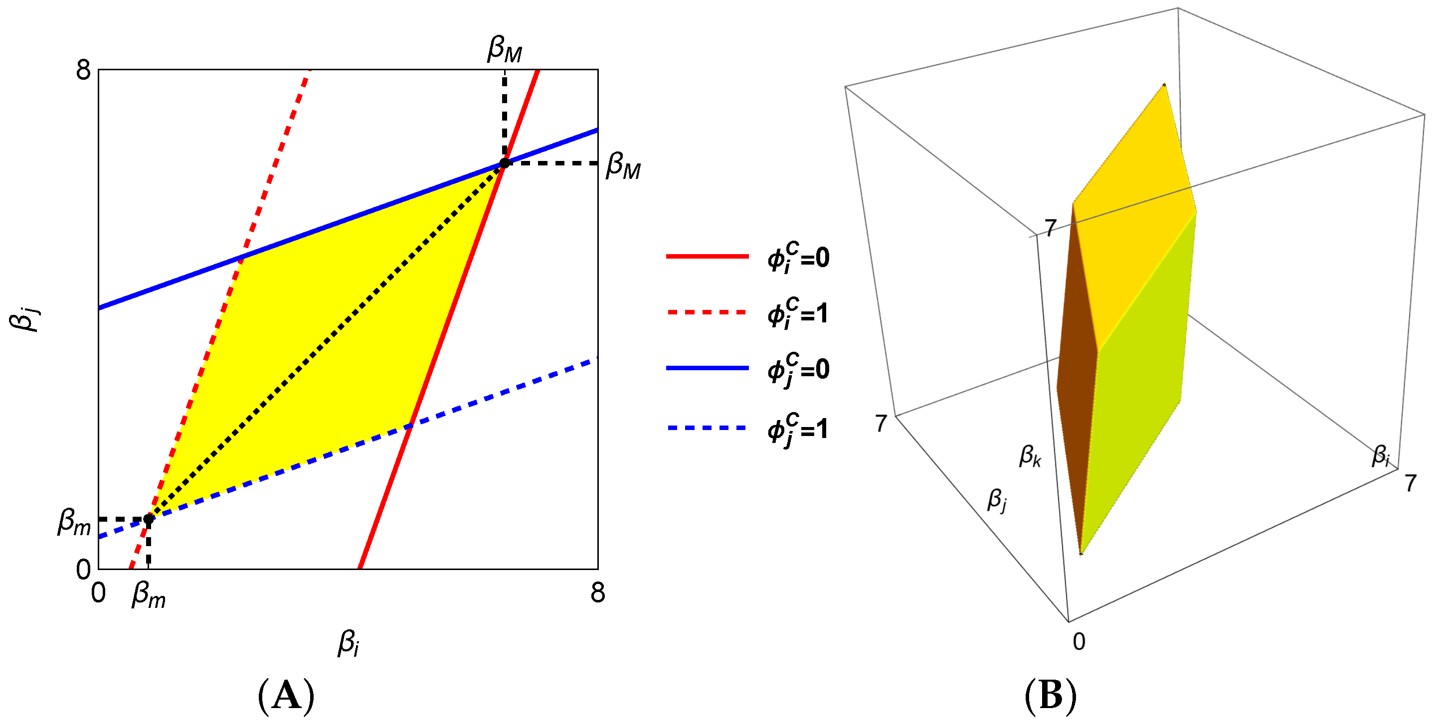
The optimal productions and optimal abatement technologies satisfy the feasible conditions, $0\le {\varphi }_k^C\le 1$ and $0\le q_k^C\le \theta /2$, if the market sizes are in the set, for $k=1,2,\dots ,n$, as follows:

$$M_n=\{\left.\left({\beta }_1,{\beta }_2,\dots {\beta }_n\right)\right|f_1\left({\beta }_k\right)\le {\beta }_{-k}\le f_0\left({\beta }_k\right)\mathrm{and}{\beta }_m\le {\beta }_k\le {\beta }_M\}$$

In the case of duopoly (i.e., $n=2$), the set $M_2$ is the diamond-shaped yellow region in Figure 1A, surrounded by the solid red and dotted red lines of ${\varphi }_i^C=0$ and ${\varphi }_i^C=1$ and by the solid blue and dotted blue lines of ${\varphi }_j^C=0$ and ${\varphi }_j^C=1.$ Notice that the solid blue and red curves intersect at ${\beta }_i={\beta }_j={\beta }_M$ and so do the dotted blue and red curves at ${\beta }_i={\beta }_j={\beta }_m$. If the two firms are homogeneous (i.e., ${\beta }_i={\beta }_j$), the feasible region is shrunk to the dotted diagonal between ${\beta }_m$ and ${\beta }_M.$ In the case of triopoly (i.e., $n=3$), the feasible region $M_3$ is described by the hexahedron with diamond-shaped faces, as seen in Figure 1B.

Figure 1. Feasible regions with $\gamma =3/5\mathrm{and}\theta =4/5$. (A) $n=2$. (B) $n=3$.

From (9) and (10), we have the following:

$$q_k^C-{\overline{q}}^C={\displaystyle \frac{2}{4-{\theta }^2-2\gamma }}({\beta }_k-\overline{\beta })$$

and

$${\varphi }_k^C-{\overline{\varphi }}^C=-{\displaystyle \frac{\theta }{2}}\left(q_k^C-{\overline{q}}^C\right)$$

where the corresponding averages are defined as

$$\overline{\beta }={\displaystyle \frac{1}{n}}{\sum }_{j=1}^n{\beta }_j,{\overline{q}}^C={\displaystyle \frac{1}{n}}{\sum }_{j=1}^n{q}_j^C\mathrm{and}{\overline{\varphi }}^C={\displaystyle \frac{1}{n}}{\sum }_{j=1}^n{\varphi }_j^C.$$

The following results concerning the optimal decisions among the firms are familiar:

Theorem 2.

Firm $k$ with a larger market size than the average produces more output and adopts more efficient abatement technology than the corresponding averages:

$${\beta }_k⋛\overline{\beta }\mathit{implies}{q}_k^C⋛{\overline{q}}^C\mathit{and}{\varphi }_k^C⋚{\overline{\varphi }}^C.$$

3. Ambient Charge Effect: Homogeneous Firms

We now turn the attention to the effects caused by a change in the ambient charge rate on the total amount of NPS pollution. Let us begin with a simple case in which the firms are homogeneous. To this end, we impose the homogeneous assumption in this section:

Assumption 3.

${\beta }_k=\beta$ for $k=1,2,\dots ,n$.

Inserting ${\beta }_k=\beta$ into (9) and (10) yields the Cournot equilibrium output and optimal abatement technology:

$$q^C\left(\theta \right)={\displaystyle \frac{2(\theta -\beta )}{4+2(n-1)\gamma +{\theta }^2}}\mathrm{and}{\varphi }^C\left(\theta \right)={\displaystyle \frac{4+2(n-1)\gamma -\beta \theta }{4+2(n-1)\gamma +{\theta }^2}}.$$

The feasibility condition, $0<{\varphi }^C<1$, is transformed as

$$\theta <\beta <{\displaystyle \frac{4+2(n-1)\gamma }{\theta }}$$

under which the Cournot output is positive and bounded above, as follows:

$$0<q^C\left(\theta \right)<{\displaystyle \frac{2}{\theta }}.$$

The total amount of production pollution is the sum of individual pollutions:

$$E_n^C\left(\theta \right)=n{\varphi }^C\left(\theta \right)q^C\left(\theta \right).$$

(17)

To see how a change in the pollution tax rate affects the total amount, we differentiate $E_n^C\left(\theta \right)$ with respect to $\theta$ and obtain, after arranging the terms, the following form of the derivative:

$${\displaystyle \frac{d{E}_n^C}{d\theta }}=-{\displaystyle \frac{2n{\phi }_n\left(\beta \right)}{{\left(4+2(n-1)\gamma -{\theta }^2\right)}^3}}$$

(18)

where ${\phi }_n\left(\beta \right)$ is quadratic in $\beta$:

$${\phi }_n\left(\beta \right)={\mathit{a}}_n{\beta }^2+{\mathit{b}}_n\beta +{\mathit{k}}_n$$

with

$${\mathit{a}}_n=4+(2n-1)\gamma +3{\theta }^2>0,$$

$${\mathit{b}}_n=-2\theta \left[12+6(n-1)\gamma -{\theta }^2\right]<0$$

$${\mathit{k}}_n=2\left[2+(n-1)\gamma \right]\left[4+2(n-1)\gamma +3{\theta }^2\right]>0.$$

Since the quadratic and constant coefficients of ${\phi }_n\left(\beta \right)$ are positive, ${\phi }_n\left(\beta \right)$ is convex in $\beta$ and ${\phi }_n\left(0\right)>0.$ Its discriminant is

$$D_{\phi }=-4{\left(4+2(n-1)\gamma -{\theta }^2\right)}^3<0.$$

Hence, ${\phi }_n\left(\beta \right)>0$ for $\beta \ge 0.$ Therefore, we have the following from (18):

Theorem 3.

Under Assumptions 1, 2, and 3, the ambient charge is effective in controlling the total amount of NPS pollution when the firms are homogeneous:

$${\displaystyle \frac{d{E}_n^C}{d\theta }}=-{\displaystyle \frac{2n\left({\mathit{a}}_n{\beta }^2+{\mathit{b}}_n\beta +{\mathit{k}}_n\right)}{{\left(4+2(n-1)\gamma -{\theta }^2\right)}^3}}<0\mathit{for}\mathit{integer}n\ge 2.$$

By continuity, the negative derivative in Theorem 3 implies that the ambient charge is still effective even if the firms are heterogeneous, provided that their heterogeneities are small enough. We will next move to the general heterogeneous firms in the following section.

4. Ambient Charge Effect: Heterogeneous Firms

We remove Assumption 3 and consider the $\theta$-effect on the total amount of NPS pollution when the firms are heterogeneous. The total amount of production pollution is the sum of the following individual pollutions:

$${\mathit{E}}_n^C\left(\theta \right)={\sum }_{k=1}^n{\varphi }_k^C\left(\theta \right)q_k^C\left(\theta \right).$$

Differentiating ${\mathit{E}}_n^C\left(\theta \right)$ with respect to $\theta$ yields the following form

$${\displaystyle \frac{d{\mathit{E}}_n^C}{d\theta }}=-{\displaystyle \frac{2F_n\left({\mathit{\beta }}_n\right)}{{\left(4+2(n-1)\gamma -{\theta }^2\right)}^3{\left(4-2\gamma -{\theta }^2\right)}^3}}$$

(19)

where ${\mathit{\beta }}_n$ is a row vector defined as

$${\mathit{\beta }}_n=\left({\beta }_1,{\beta }_2,\dots ,{\beta }_n\right),$$

and $F_n\left({\mathit{\beta }}_n\right)$ in the denominator of (19) is

$$F_n\left({\mathit{\beta }}_n\right)=A_n{\sum }_{k=1}^n{\beta }_k^2+B_n{\sum }_{k=1}^n{\beta }_k+C_n{\sum }_{k=1}^{n-1}{\sum }_{j=k+1}^n{\beta }_k{\beta }_j+K_n$$

(20)

and the parametric forms of $A_n,B_n$, $C_n$ and $K_n$ are given in Appendix A as they are too long to be presented here. Furthermore, it is demonstrated in the Results A1 and A2 that under Assumptions 1 and 2,

$$A_n>0,B_n<0,C_n<0\mathrm{and}{K}_n>0\mathrm{for}\mathrm{any}n\ge 2$$

The right-hand side form of (20) is rewritten as the sum of the quadratic polynomials for $k=1,2,\dots ,n-2$, as shown below. If we have to have uniformity of notation, $F_n\left({\mathit{\beta }}_n\right)$ should be $F_n^n\left({\mathit{\beta }}_n\right)$:

$$\begin{array}{c}{F}_n\left({\mathit{\beta }}_n\right)=A_n{\beta }_n^2+\left(B_n+C_n{\displaystyle \sum _{i=1}^{n-1}}{\beta }_i\right){\beta }_n+F_n^{n-1}\left({\mathit{\beta }}_{n-1}\right),\hfill \\ F_n^{n-k}\left({\mathit{\beta }}_{n-k}\right)=A_n{\beta }_{n-k}^2+\left(B_n+C_n{\displaystyle \sum _{i=1}^{n-k}}{\beta }_i\right){\beta }_{n-k}+F_n^{n-(k+1)}\left({\mathit{\beta }}_{n-(k+1)}\right),\hfill \\ F_n^1\left({\beta }_1\right)=A_n{\beta }_1^2+B_n{\beta }_1+K_n\hfill \end{array}$$

(21)

where $A_n>0$ implies that $F_n\left({\mathit{\beta }}_n\right)$ is convex in ${\beta }_n$ and so are $F_n^{n-k}\left({\mathit{\beta }}_{n-k}\right)$ in ${\beta }_{n-k}$ for $k=1,2,\dots ,n-1$. We aim to show $F_n\left({\mathit{\beta }}_n\right)>0$ for $n\ge 2$, with which the derivative (19) is negative since its denominator and numerator are positive for any $n\ge 2$. However, the form in (20) is too complex to determine its sign, so we start with the most simplified case in Section 4.1, where the firms are duopoly. We then consider the triopoly firms in Section 4.2 and move to a general oligopoly in Section 4.3 to show, first, that $F_n^{n-k}\left({\mathit{\beta }}_{n-k}\right)>0$ for ${\mathit{\beta }}_{n-k}\ge 0$ for each $k=1,2,\dots ,k-1$, and secondly that $F_n\left({\mathit{\beta }}_n\right)>0$ for ${\beta }_n$.

4.1. Duopoly: $n=2$

We begin with a duopoly case. Substituting $n=2$ into (21) yields

$$F_2({\beta }_1,{\beta }_2)=A_2{\beta }_2^2+\left(B_2+C_2{\beta }_1\right){\beta }_2+F_2^1\left({\beta }_1\right)$$

(22)

with

$$F_2^1\left({\beta }_1\right)=A_2{\beta }_1^2+B_2{\beta }_1+K_2.$$

(23)

The parameters have the following forms:

$$\begin{array}{c}{A}_2=16(4-{\gamma }^2)(4+{\gamma }^2)+192{\gamma }^2{\theta }^2-48(2+{\gamma }^2){\theta }^4+\left(32-3{\theta }^2\right){\theta }^4,\hfill \\ B_2=-2\theta (12+6\gamma +{\theta }^2){(4-2\gamma -{\theta }^2)}^3,\hfill \\ C_2=-8\gamma \left[16(4-{\gamma }^2)+12(4+{\gamma }^2){\theta }^2-36{\theta }^4+5{\theta }^6\right],\hfill \\ K_2=4(2+\gamma )(4+2\gamma +3{\theta }^2){(4-2\gamma -{\theta }^2)}^3.\hfill \end{array}$$

(24)

In this subsection, we will demonstrate first that $F_2^1\left({\beta }_1\right)>0$ for ${\beta }_1\ge 0$ and then that $F_2({\beta }_1,{\beta }_2)>0$ for ${\beta }_1\ge 0$ and ${\beta }_2\ge 0$.

$F_2({\beta }_1,{\beta }_2)$ in (22) is quadratic in ${\beta }_2$, and its discriminant is

$$D_{F_2}\left({\beta }_1\right)={\left(B_2+C_2{\beta }_1\right)}^2-4A_2{F}_2^1\left({\beta }_1\right).$$

Using (23) allows us to rewrite $D_{F_2}\left({\beta }_1\right)$ as

$$D_{F_2}\left({\beta }_1\right)=-\left(4A_2^2-C_2^2\right){\beta }_1^2-2B_2(2A_2-C_2){\beta }_1+D_{F_2^1}(\gamma ,\theta ).$$

(25)

Here, $D_{F_2^1}(\gamma ,\theta )$ denotes the discriminant of $F_2^1\left({\beta }_1\right)$ as follows:

$$D_{F_2^1}(\gamma ,\theta )=B_2^2-4A_2{K}_2.$$

We first focus on $F_2^1\left({\beta }_1\right)$:

Lemma 1.

Under Assumptions 1 and 2, $F_2^1\left({\beta }_1\right)>0$ for any ${\beta }_1\ge 0$.

Proof. 

With the parameters in (24), the discriminant of $F_2^1\left({\beta }_1\right)$ is expanded as

$$D_{F_2^1}(\gamma ,\theta )=-4{(4+2\gamma -{\theta }^2)}^3{(4-2\gamma -{\theta }^2)}^3{g}_2^1(\gamma ,\theta )$$

where $4+2\gamma -{\theta }^2>0,4-2\gamma -{\theta }^2>0$ and

$$g_2^1(\gamma ,\theta )=16(2-\gamma )(4+{\gamma }^2)+12(4+8\gamma -{\gamma }^2){\theta }^2+\left[12(4+\gamma )-{\theta }^2\right]{\theta }^4>0.$$

Hence, $D_{F_2^1}(\gamma ,\theta )<0$. $F_2^1\left({\beta }_1\right)$ with $A_2>0$ is convex in ${\beta }_1$ and $F_2^1\left(0\right)=K_2>0$. Therefore, $F_2^1\left({\beta }_1\right)>0$ for any ${\beta }_1\ge 0$. This completes the proof. □

We now turn to show $F_2({\beta }_1,{\beta }_2)>0$:

Lemma 2.

$F_2({\beta }_1,{\beta }_2)>0$ for ${\beta }_1\ge 0$ and ${\beta }_2\ge 0$.

Proof. 

As is seen in (25), the discriminant of $F_2({\beta }_1,{\beta }_2)$ is quadratic in ${\beta }_1$. Let us denote the right-hand form of (25) by $f_2\left({\beta }_1\right)$ for simplicity. The bracketed part of the quadratic coefficient of $f_2\left({\beta }_1\right)$ is positive because it is factorized, as follows:

$$4A_2^2-C_2^2=\left(2A_2-C_2\right)\left(2A_2+C_2\right)$$

where $2A_2-C_2>0$ and

$$2A_2+C_2=2\left(4+2\gamma +3{\theta }^2\right){\left(4-2\gamma -{\theta }^2\right)}^3>0.$$

Hence, $f_2\left({\beta }_1\right)$ is concave in ${\beta }_1$ and $f_2\left(0\right)=D_{F_2^1}(\gamma ,\theta )<0$ due to Lemma 1. Then, the discriminant of $f_2\left({\beta }_1\right)$ with respect to ${\beta }_1$ is

$$\begin{array}{cc}\hfill D_{f_2}(\gamma ,\theta )/4& =B_2^2{(2A_2-C_2)}^2+\left(4A_2^2-C_2^2\right)D_{F_2^1}(\gamma ,\theta )\hfill \\ \hfill & =-4A_2(2A_2-C_2)\left[\left(2A_2+C_2\right)K_2-B_2^2\right]\hfill \end{array}$$

where the square-bracketed term in the second line is positive:

$$\left(2A_2+C_2\right)K_2-B_2^2=4{(4+2\gamma -{\theta }^2)}^3{(4-2\gamma -{\theta }^2)}^3>0.$$

Thus, $D_{f_2}(\gamma ,\theta )<0$, which then implies $f_2\left({\beta }_1\right)=D_{F_2}\left({\beta }_1\right)<0$ for ${\beta }_1\ge 0$. With $A_2>0$, $F_2({\beta }_1,{\beta }_2)$ is convex in ${\beta }_2$, and $F_2({\beta }_1,0)=F_2^1\left({\beta }_1\right)>0$ due to Lemma 1. Therefore, the negative discriminant implies $F_2({\beta }_1,{\beta }_2)>0$ for ${\beta }_1\ge 0$ and ${\beta }_2\ge 0$. This completes the proof. □

The denominator of Equation (19) is positive due to Assumptions 1 and 2. Hence, Lemma 2 immediately yields the following:

Theorem 4.

Given Assumptions 1 and 2, the ambient charge is effective in controlling the total amount of NPS pollution when the market is in duopoly (i.e., $n=2$):

$${\displaystyle \frac{d{\mathit{E}}_2^C}{d\theta }}=-{\displaystyle \frac{2F_2({\beta }_1,{\beta }_2)}{{\left(4+2\gamma -{\theta }^2\right)}^3{\left(4-2\gamma -{\theta }^2\right)}^3}}<0.$$

4.2. Triopoly: $n=3$

Substituting $n=3$ into (21) yields

$$F_3({\beta }_1,{\beta }_2,{\beta }_3)=A_3{\beta }_3^2+\left[B_3+C_3\left({\beta }_1+{\beta }_2\right)\right]{\beta }_3+F_3^2({\beta }_1,{\beta }_2),$$

$$F_3^2({\beta }_1,{\beta }_2)=A_3{\beta }_2^2+\left(B_3+C_3{\beta }_1\right){\beta }_2+F_3^1\left({\beta }_1\right),$$

$$F_3^1\left({\beta }_1\right)=A_3{\beta }_1^2+B_3{\beta }_1+K_3.$$

Here, the parameters are

$$\begin{array}{c}{A}_3=32(2-\gamma )(1+\gamma )(4+4\gamma +3{\gamma }^2)+24\left(4+20\gamma +7{\gamma }^2\right){\theta }^2\hfill \\ -12(8+10\gamma +11{\gamma }^2){\theta }^4+\left[\left(32+18\gamma \right)-3{\theta }^2\right]{\theta }^4,\hfill \\ B_3=-2\theta (12+12\gamma +{\theta }^2){(4-2\gamma -{\theta }^2)}^3,\hfill \\ C_3=-8\gamma \left[8(1+\gamma )(2-\gamma )(4+\gamma )+6(8+4\gamma +5{\gamma }^2){\theta }^2-9(4+\gamma ){\theta }^4+5{\theta }^6\right],\hfill \\ K_3=12(1+\gamma )(4+4\gamma +3{\theta }^2){(4-2\gamma -{\theta }^2)}^3.\hfill \end{array}$$

$F_3({\beta }_1,{\beta }_2,{\beta }_3),F_3^2({\beta }_1,{\beta }_2)$ and $F_3^1\left({\beta }_1\right)$ are quadratic in ${\beta }_3,{\beta }_2$ and ${\beta }_1$, respectively. Their discriminants are

$$D_{F_3}({\beta }_1,{\beta }_2)={\left[B_3+C_3\left({\beta }_1+{\beta }_2\right)\right]}^2-4A_3{F}_3^2({\beta }_1,{\beta }_2)$$

$$D_{F_3^2}\left({\beta }_1\right)={\left(B_3+C_3{\beta }_1\right)}^2-4A_3{F}_3^1\left({\beta }_1\right)$$

and

$$D_{F_3^1}(\gamma ,\theta )=B_3^2-4A_3{K}_3.$$

Repeating the procedure taken in the case of $n=2,$ we will sequentially show the controllability of the ambient charge as follows:

$$\begin{array}{c}\mathrm{Lemma}3:D_{F_3^1}(\gamma ,\theta )<0\Rightarrow F_3^1\left({\beta }_1\right)>0;\hfill \\ \mathrm{Lemma}4:D_{F_3^1}(\gamma ,\theta )<0\mathrm{and}{D}_{F_3^2}\left({\beta }_1\right)<0\Rightarrow F_3^2({\beta }_1,{\beta }_2)>0;\hfill \\ \mathrm{Lemma}5:D_{F_3^2}\left({\beta }_1\right)<0\mathrm{and}{D}_{F_3}({\beta }_1,{\beta }_2)<0\Rightarrow F_3({\beta }_1,{\beta }_2,{\beta }_3)>0.\hfill \end{array}$$

Lemma 3.

Under Assumptions 1 and 2, $F_3^1\left({\beta }_1\right)>0$ for any ${\beta }_1\ge 0$.

Proof. 

The discriminant of $F_3^1\left({\beta }_1\right)$ is expanded as

$$D_{F_3^1}(\gamma ,\theta )=-4{(4+2\gamma -{\theta }^2)}^3{(4-2\gamma -{\theta }^2)}^3{g}_3^1(\gamma ,\theta )$$

where $4+2\gamma -{\theta }^2>0$, $4-2\gamma -{\theta }^2>0$, and, under Assumptions 1 and 2,

$$g_3^1(\gamma ,\theta )=24(2-\gamma )(4+4\gamma +3{\gamma }^2)+36(4+8\gamma +{\gamma }^2){\theta }^2+\left[6(14+11\gamma )-{\theta }^2\right]{\theta }^4>0.$$

Hence, $D_{F_3^1}(\gamma ,\theta )<0$. $F_3^1\left({\beta }_1\right)$ is convex in ${\beta }_1$ and $F_3^1\left(0\right)=K_3>0$. Therefore, $F_3^1\left({\beta }_1\right)>0$ for any ${\beta }_1\ge 0$. This completes the proof. □

Lemma 4.

Under Assumptions 1 and 2$,F_3^2({\beta }_1,{\beta }_2)>0$ for ${\beta }_1\ge 0$ and ${\beta }_2\ge 0$.

Proof. 

The discriminant of $F_3^2({\beta }_1,{\beta }_2)$ is rewritten as

$$D_{F_3^2}\left({\beta }_1\right)=-(4A_3^2-C_3^2){\beta }_1^2-2B_3(2A_3-C_3){\beta }_1+D_{F_3^1}(\gamma ,\theta )$$

where the quadratic coefficient is negative as $2A_3-C_3>0$ and $2A_3+C_3>0$ is numerically confirmed, as shown below. This term is confirmed to be negative under Assumptions 1 and 2.

$$2A_3+C_3=2\left(m_0+m_2{\theta }^2+m_4{\theta }^4+m_6{\theta }^6+3{\theta }^8\right)>0$$

where

$$\begin{array}{c}{m}_0=64(1+\gamma )(2-\gamma )(2+{\gamma }^2),\hfill \\ m_2=-48\gamma (2-8\gamma -{\gamma }^2),\hfill \\ m_4=-24(4-\gamma -4{\gamma }^2),\hfill \\ m_6=2(16-\gamma ).\hfill \end{array}$$

Meanwhile, the constant term $D_{F_3^1}(\gamma ,\theta )$ is negative due to Lemma 3. Let $f_3^2\left({\beta }_1\right)$ be the right-hand side form of the above equation. It is quadratic in ${\beta }_1$, and its discriminant is

$$\begin{array}{cc}\hfill D_{f_3^2}(\gamma ,\theta )/4& =B_3^2{(2A_3-C_3)}^2+\left(4A_3^2-C_3^2\right)D_{F_3^1}(\gamma ,\theta )\hfill \\ \hfill & =-4A_3(2A_3-C_3)\left[(2A_3+C_3)K_3-B_3^2\right]\hfill \end{array}$$

where the square-bracketed term is

$$(2A_3+C_3)K_3-B_3^2=4{(4+4\gamma -{\theta }^2)}^3{(4-2\gamma -{\theta }^2)}^3{g}_3^2(\gamma ,\theta )$$

and

$$g_3^2(\gamma ,\theta )=24(2-\gamma )\left(2+{\gamma }^2\right)+108\gamma {\theta }^2+\left[6(5+2\gamma )-{\theta }^2\right]{\theta }^4>0.$$

Hence, $D_{f_3^2}(\gamma ,\theta )<0$. Since $f_3^2\left({\beta }_1\right)$ is concave in ${\beta }_1$ and $f_3^2\left(0\right)=D_{F_3^1}(\gamma ,\theta )<0$ due to Lemma 3, $f_3^2\left({\beta }_1\right)=D_{F_3^2}\left({\beta }_1\right)<0$ for all ${\beta }_1\ge 0$. With the negative discriminant and convexity in ${\beta }_2$, $F_3^2({\beta }_1,{\beta }_2)>0$ for ${\beta }_1\ge 0$ and ${\beta }_2\ge 0$. This completes the proof. □

Having Lemmas 3 and 4, we now turn the attention to the parametric conditions under which $F_3({\beta }_1,{\beta }_2,{\beta }_3)$ is positive.

Lemma 5.

Under Assumptions 1 and 2, $F_3({\beta }_1,{\beta }_2,{\beta }_3)>0$ for any ${\beta }_1\ge 0,{\beta }_2\ge 0$ and ${\beta }_3\ge 0$.

Proof. 

The discriminant of $F_3({\beta }_1,{\beta }_2,{\beta }_3)>0$ is quadratic in ${\beta }_2$:

$$D_{F_3}({\beta }_1,{\beta }_2)=-(4A_3^2-C_3^2){\beta }_2^2-2(2A_3-C_3)\left(B_3+C_3{\beta }_1\right){\beta }_2+D_{F_3^2}\left({\beta }_1\right)$$

where the quadratic coefficient is negative and the constant term is negative due to Lemma 4. $D_{F_3}({\beta }_1,{\beta }_2)$ is concave in ${\beta }_2$. Thus, if $D_{F_3}({\beta }_1,{\beta }_2)<0$, then $F_3({\beta }_1,{\beta }_2,{\beta }_3)>0$. We show the negative discriminant with three steps:

[i] For notational simplicity, $f_3^2({\beta }_1,{\beta }_2)=D_{F_3}({\beta }_1,{\beta }_2).$ It is concave in ${\beta }_2$ and $f_3^2({\beta }_1,0)=D_{F_3^2}\left({\beta }_1\right)<0$. Its discriminant for ${\beta }_2$ is

$$\begin{array}{cc}{D}_{f_3^2}\left({\beta }_1\right)/4\hfill & ={(2A_3-C_3)}^2{\left(B_3+C_3{\beta }_1\right)}^2+\left(4A_3^2-C_3^2\right)D_{F_3^2}\left({\beta }_1\right),\hfill \\ & =-4A_3(2A_3-C_3)f_3^1\left({\beta }_1\right)\hfill \end{array}$$

where

$$f_3^1\left({\beta }_1\right)=(2A_3-C_3)(A_3+C_3){\beta }_1^2+B_3(2A_3-C_3){\beta }_1+\left[(2A_3-C_3)K_3-B_3^2\right]$$

The quadratic coefficient is positive as $2A_3-C_3>0$ and

$$A_3+C_3=(4-2\gamma -{\theta }^2)(4+4\gamma +3{\theta }^2)>0.$$

The square-bracketed constant term is also positive:

$$(2A_3-C_3)K_3-B_3^2=4{(4+4\gamma -{\theta }^2)}^3{(4-2\gamma -{\theta }^2)}^3>0.$$

$f_3^1\left({\beta }_1\right)$ is convex in ${\beta }_1$. Hence, if its discriminant is negative, then $f_3^1\left({\beta }_1\right)>0$.

[ii] The discriminant of  $f_3^1\left({\beta }_1\right)$ is

$$\begin{array}{cc}{D}_{f_3^1}(\gamma ,\theta )\hfill & =B_3^2{(2A_3-C_3)}^2-4(2A_3-C_3)(A_3+C_3)\left[(2A_3-C_3)K_3-B_3^2\right],\hfill \\ & =-(2A_3^2-C_3^2)\left[4(A_3+C_3)K_3-3B_3^2\right].\hfill \end{array}$$

The first factor in the form on the right-hand side of the second line is positive, $2A_3^2-C_3^2>0,$ and the square-bracketed factor is also positive:

$$4(A_3+C_3)K_3-3B_3^2=12{(4+4\gamma -{\theta }^2)}^3{(4-2\gamma +{\theta }^2)}^6>0.$$

Hence, $D_{f_3^1}(\gamma ,\theta )<0$, which then implies $D_{F_3}({\beta }_1,{\beta }_2)<0$.

[iii] We now arrive at the main conclusion through the following chain of the results:

$$\begin{array}{c}1.D_{f_3}(\gamma ,\theta )<0\Rightarrow f_3^1\left({\beta }_1\right)>0\mathrm{for}\mathrm{any}{\beta }_1\ge 0;\hfill \\ 2.f_3^1\left({\beta }_1\right)>0\Rightarrow D_{f_3^2}\left({\beta }_1\right)<0;\hfill \\ 3.D_{f_3^2}\left({\beta }_1\right)<0\Rightarrow f_3^2({\beta }_1,{\beta }_2)=D_{F_3}({\beta }_1,{\beta }_2)<0\mathrm{for}{\beta }_1\ge 0\mathrm{and}{\beta }_2\ge 0;\hfill \\ 4.D_{F_3}({\beta }_1,{\beta }_2)<0\Rightarrow F_3({\beta }_1,{\beta }_2,{\beta }_3)>0\mathrm{for}{\beta }_1\ge 0,{\beta }_2\ge 0\mathrm{and}{\beta }_3\ge 0.\hfill \end{array}$$

This completes the proof. □

With these lemmas for $n=3$, we arrive at the following result:

Theorem 5.

Given Assumptions 1 and 2, the ambient charge is effective in controlling the total amount of NPS pollution when the market is triopoly:

$${\displaystyle \frac{d{\mathit{E}}_3^C}{d\theta }}=-{\displaystyle \frac{2F_3({\beta }_1,{\beta }_2,{\beta }_3)}{{\left(4+4\gamma -{\theta }^2\right)}^3{\left(4-2\gamma -{\theta }^2\right)}^3}}<0.$$

4.3. Numerical Analysis

Following the same procedure to be used above, we can show the effectiveness of the ambient tax policy for any n. Returning to polynimials in (21), we notice that $A_n>0$ implies that $F_n^{n-k}\left({\mathit{\beta }}_{n-k}\right)$ is convex in ${\beta }_{n-k}$ for $k=1,2,\dots ,n-1$. If its discriminant is negative, then $F_n^{n-k}\left({\mathit{\beta }}_{n-k}\right)>0$ for ${\mathit{\beta }}_{n-k}\ge 0$. With $F_n^{n-1}\left({\mathit{\beta }}_{n-1}\right)>0$ for ${\mathit{\beta }}_{n-1}\ge 0$, it also can be shown that $F_n\left({\mathit{\beta }}_n\right)$ is convex in ${\beta }_n$ and its discriminant is negative. Hence, $F_n\left({\mathit{\beta }}_n\right)>0$ for any ${\mathit{\beta }}_n\ge 0$. Therefore, we can arrive at our final destination:

$${\displaystyle \frac{d{\mathit{E}}_n^C}{d\theta }}<0\mathrm{for}\mathrm{any}n\ge 2.$$

However, as the saying goes, “easier said than done”. The proof for the controllability of the ambient charge becomes longer and clumsy as n increases. Instead of repeating the tedious procedure, we graphically confirm the effectiveness of the tax policy in the case of $n\ge 4$ at the expense of mathematical rigor. In graphical analysis, we treat ${\beta }_1$ and ${\beta }_2$ as variables and the remaining ${\beta }_j$s as being constant only for convenience. To this end, we reformulate the third term of (20):

$$C_n{\sum }_{k=1}^{n-1}{\sum }_{j=k+1}^n{\beta }_k{\beta }_j=C_n\left[{\beta }_1{\beta }_2+\left({\beta }_1+{\beta }_2\right){\sum }_{k=3}^n{\beta }_k+{\sum }_{k=3}^{n-1}{\sum }_{j=k+1}^n{\beta }_k{\beta }_j\right].$$

Accordingly, $F_n\left({\beta }_n\right)$ is rewritten as

$$F_n\left({\mathit{\beta }}_n\right)=A_n({\beta }_1^2+{\beta }_2^2)+\left(B_n+C_n{\sum }_{k=3}^n{\beta }_k\right)({\beta }_1+{\beta }_2)+C_n{\beta }_1{\beta }_2+G_n\left({\overline{\mathit{\beta }}}_n\right)$$

(26)

where $G_n\left({\overline{\mathit{\beta }}}_n\right)$ is a constant term and has the following form:

$$G_n\left({\overline{\mathit{\beta }}}_n\right)=A_n{\sum }_{k=3}^n{\beta }_k^2+B_n{\sum }_{k=3}^n{\beta }_k+C_n{\sum }_{k=3}^{n-1}{\sum }_{j=k+1}^n{\beta }_k{\beta }_j+K_n$$

and

$${\overline{\mathit{\beta }}}_n=({\beta }_3,{\beta }_4,\dots ,{\beta }_n).$$

To proceed to the graphical analysis, we first specify the values of $\gamma$ and $\theta$, as shown below. Any numbers satisfying $0<\gamma <1$ and $0<\theta <\sqrt{2}$ are possible.

Assumption 4.

$\gamma =4/5$ and $\theta =1$.

Polynominal (26) is essentially quadratic in ${\beta }_1$ and ${\beta }_2$. Before proceeding to the case of $n\ge 4$, we graphically examine the $n=2$ case, which we have already analytically considered in Lemma 2. Polynomials (22) and (23) or (26) with $n=2$ lead to

$$F_2({\beta }_1,{\beta }_2)=A_2({\beta }_1^2+{\beta }_2^2)+B_2({\beta }_1+{\beta }_2)+C_4{\beta }_1{\beta }_2+K_2$$

(27)

where Assumption 4 specifies the parameter values given in (24) as

$$A_2={\displaystyle \frac{171629}{625}},B_2=-{\displaystyle \frac{61054}{625}},C_2=-{\displaystyle \frac{62752}{125}},K_2={\displaystyle \frac{825944}{3125}}.$$

Figure 2A illustrates the graph of $F_2({\beta }_1,{\beta }_2)$ in which $F_2({\beta }_1,{\beta }_2)>0$ for $0\le {\beta }_i\le 4$ for $i=1,2$. It is suggested that $F_2({\beta }_1,{\beta }_2)>0$ could hold for any ${\beta }_i\ge 0$. Figure 2A graphically confirms Lemma 2. Furthermore, the derivative in (19) for $n=2$ is approximated as

$${\displaystyle \frac{d{\mathit{E}}_2^C}{d\theta }}\simeq -2.06({\beta }_1^2+{\beta }_2^2)+0.73({\beta }_1+{\beta }_2)+3.76{\beta }_1{\beta }_2-1.98.$$

The maximands of ${\beta }_1$ and ${\beta }_2$ as well as the corresponding maximum value of $d{E}_2^C/d\theta$ are

$${\beta }_1^m={\beta }_2^m={\displaystyle \frac{89}{43}}\simeq 2.07\mathrm{and}{\left.{\displaystyle \frac{d{\mathit{E}}_2^C}{d\theta }}\right|}_{{\beta }_1={\beta }_1^m,{\beta }_2={\beta }_2^m}=-{\displaystyle \frac{20}{43}}\simeq -0.47.$$

Figure 2B is the graph of $d{E}_2^C/d\theta$ and shows that it is negative over the same domain, and the red point denotes the maximum value, which is negative.

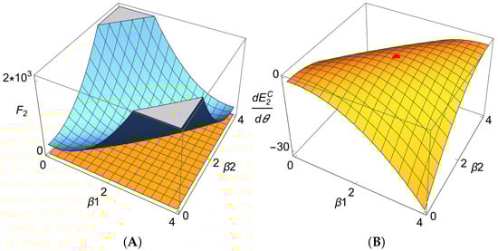
Figure 2. The ambient charge effect for n = 2. (A) Graph of $F_2({\beta }_1,{\beta }_2)$. (B) Graph of $d{E}_2^C/d\theta$.

We now move on to polynominal (26) with $n=4$:

$$F_4({\beta }_1,{\beta }_2,{\beta }_3,{\beta }_4)=A_4({\beta }_1^2+{\beta }_2^2)+\left[B_4+C_4\left({\beta }_3+{\beta }_4\right)\right]({\beta }_1+{\beta }_2)+C_4{\beta }_1{\beta }_2+G_4({\beta }_3,{\beta }_4)$$

and

$$G_4({\beta }_3,{\beta }_4)=A_4({\beta }_3^2+{\beta }_4^2)+B_4({\beta }_3+{\beta }_4)+C_4{\beta }_3{\beta }_4+K_4$$

where parameters $A_4,B_4,C_4$ and $K_4$ are

$$A_4={\displaystyle \frac{1206269}{625}}\simeq 1930,B_4=-{\displaystyle \frac{93982}{625}}\simeq -150,$$

$$C_4=-{\displaystyle \frac{790688}{625}}\simeq -1265,K_4={\displaystyle \frac{35617212}{3125}}\simeq 1140.$$

It is clear that changing values of ${\beta }_3$ and ${\beta }_4$ shifts the graph of $F_4({\beta }_1,{\beta }_2,{\beta }_3,{\beta }_4)$ but does not affect its shape, which depends only on specified values of ${\beta }_1$ and ${\beta }_2$. Taking ${\beta }_3={\beta }_4=2$ gives rise to a numerical form of $F_4({\beta }_1,{\beta }_2,{\beta }_3,{\beta }_4)$:

$$F_4({\beta }_1,{\beta }_2,{\beta }_3,{\beta }_4)={\displaystyle \frac{1206269}{625}}({\beta }_1^2+{\beta }_2^2)-{\displaystyle \frac{3256734}{625}}({\beta }_1+{\beta }_2)-{\displaystyle \frac{790688}{625}}{\beta }_1{\beta }_2+{\displaystyle \frac{34119072}{3125}}.$$

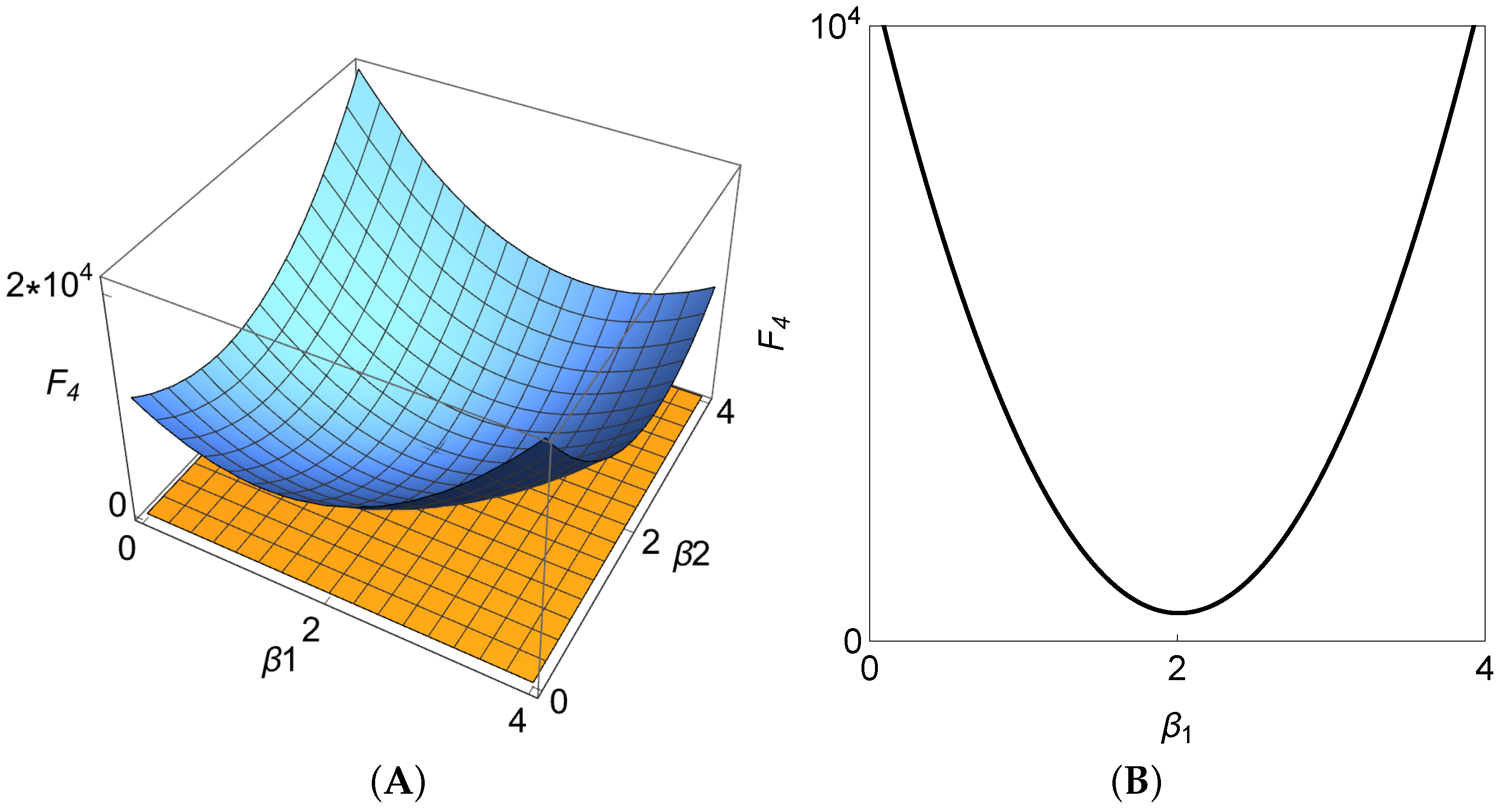
Notice that this form is essentially the same as (27)$.$Figure 3A illustrates the graph of $F_4({\beta }_1,{\beta }_2,{\beta }_3,{\beta }_4)$, in which the zero surface is in orange and the blue graph is located above the zero surface. Hence, we graphically verify the following:

$$F_4({\beta }_1,{\beta }_2,{\beta }_3,{\beta }_4)>0\mathrm{for}0\le {\beta }_i\le 4\mathrm{for}i=1,2\mathrm{and}{\beta }_3={\beta }_4=2$$

which then leads to the effectiveness of the ambient charge, which is

$${\displaystyle \frac{d{\mathit{E}}_4^C}{d\theta }}=-{\displaystyle \frac{2F_4({\beta }_1,{\beta }_2,{\beta }_3,{\beta }_4)}{{\left(4+4\gamma -{\theta }^2\right)}^3{\left(4-2\gamma -{\theta }^2\right)}^3}}<0.$$

In addition, Figure 3B illustrates the graph of $F_4\left({\mathit{\beta }}_4\right)$ with $0\le {\beta }_1={\beta }_2\le 4$ and ${\beta }_i=2$ for $i=3,4$. That is, Figure 3B is a cross-sectional view of Figure 3A that is cut diagonally. We must emphasize that the effective result is obtained under numerically specified circumstances and does not imply that it holds generally.

Figure 3. $\mathrm{Graphs}\mathrm{of}{F}_4\left({\mathit{\beta }}_4\right)\mathrm{when}\mathrm{the}\mathrm{firms}\mathrm{are}\mathrm{hetero}\text{-}\mathrm{or}\mathrm{homogeneous}$. (A) Heterogeneous: ${\beta }_1\ne {\beta }_2$. (B) Homogeneous: ${\beta }_1={\beta }_2$.

We now show that $F_5\left({\mathit{\beta }}_5\right)>F_4\left({\mathit{\beta }}_4\right)$, implying $F_5\left({\mathit{\beta }}_5\right)>0$ for ${\mathit{\beta }}_5\ge 0.$ Let $\Delta F$ be a difference of $F_5\left({\mathit{\beta }}_5\right)$ from $F_4\left({\mathit{\beta }}_4\right)$. Using (26), $\Delta F$ has the following form:

$$\Delta F=\Delta A\left({\beta }_1^2+{\beta }_2^2\right)+\left(\Delta B+\Delta C+C_5{\beta }_4\right)\left({\beta }_1+{\beta }_2\right)+\Delta C{\beta }_1{\beta }_2+\Delta G,$$

where $\Delta A=A_5-A_4,\Delta B=B_5-B_4,\Delta C=C_5-C_4,$ and $\Delta G=G_5({\beta }_3,{\beta }_4,{\beta }_5)-G_4({\beta }_3,{\beta }_4)$,

$$\Delta G=\Delta A\left({\beta }_1^2+{\beta }_2^2\right)+\left(\Delta B+\Delta C+C_5{\beta }_4\right)\left({\beta }_3+{\beta }_4\right)+\Delta C{\beta }_3{\beta }_4+\Delta g,$$

and

$$\Delta g\left({\beta }_5\right)=A_5{\beta }_5^2+B_5{\beta }_5+\Delta K$$

with $\Delta K=K_5-K_4$. Result A2 in Appendix A has already shown that $A_{k+1}-A_K>0$ and $C_{k+1}-C_K<0$ for any $k\ge 2$, implying $\Delta A>0$ and $\Delta C<0$. In addition,

$$\begin{array}{cc}\hfill B_{k+1}-B_k& =-12\gamma \theta (4-2\gamma -{\theta }^2)<0\hfill \\ \hfill K_{k+1}-K_k& =4(4-2\gamma -{\theta }^2)\left[(3k-1)k{\gamma }^2+4(1+2k\gamma )+3(1+g\gamma ){\gamma }^2\right]>0.\hfill \end{array}$$

Hence,

$$\Delta B<0\mathrm{and}\Delta K>0.$$

These sign conditions reveal that $\Delta F$ and $\Delta G$ have the same structure of polynomials (22) and that $\Delta g$ is similar to (23). $\Delta g$ is convex ${\beta }_5$, and $\Delta g\left(0\right)=\Delta K>0$, implying $\Delta g\left({\beta }_5\right)>0$ for any ${\beta }_5\ge 0$. Then, applying Lemma 2, we can show that $\Delta G>0$ for ${\beta }_3\ge 0$ and ${\beta }_4\ge 0$, and then $\Delta F>0$ for ${\beta }_1\ge 0$ and ${\beta }_2\ge 0.$ Finally, $F_4\left({\mathit{\beta }}_4\right)>0$ for ${\mathit{\beta }}_5\ge 0$ leads to

$$F_5\left({\mathit{\beta }}_5\right)>0\mathrm{for}{\mathit{\beta }}_5\ge 0.$$

Only for analytical simplicity, we impose Assumption 4 and use the dependency of the graphical result, $F_4\left({\mathit{\beta }}_4\right)>0$, to derive $F_5\left({\mathit{\beta }}_5\right)>0$. We emphasize again that $F_5\left({\mathit{\beta }}_5\right)>0$ is derived based on the numerical result of $F_4\left({\mathit{\beta }}_4\right)>0$ and is a numerically specified result.

5. Concluding Remarks

This paper develops an n-firm Cournot oligopoly model in which NPS pollution is created as a by-product of production activities and examines whether the ambient charge environmental policy controls NPS pollution. The profit-maximizing firms game-theoretically determine optimal outputs and select optimal abatement technology. Theorem 1 provides the feasibility conditions that ensure a positive output (i.e., $q_k^C>0$) and an appropriate technology (i.e., $0<{\phi }_k^C<1$) at a Nash equilibrium. Theorem 2 clarifies the dependency of optimal decisions on the market size and shows that the firm with the larger market size produces more output and more efficient technology than the corresponding market averages. Theorem 3 shows that the ambient charge scheme effectively controls NPS pollution if the firms are homogeneous in the sense that the market sizes are identical. When the firms are heterogeneous, Theorems 4 and 5 analytically demonstrate the effectiveness of the policy for duopoly ($n=2$) and triopoly ($n=3$). To proceed further, we specify the parameter values and then numerically confirm the policy effectiveness for quadopoly ($n=4$). Further, using the results in quadopoly can lead to the same result for pentopoly ($n=5$). In principle, policy effectiveness should be obtained by repeating the procedure performed in duopoly and triopoly at the expense of long and clumsy operations. Although the numerical analysis performed in quadopoly and pentopoly effectively avoids the repetition of complicated operations, the generality of the results is not guaranteed.

There are many ways to proceed from here. Determining the optimal tax rate is not discussed in this study but is an issue that needs to be considered urgently. However, efficient manipulation of complex mathematical expressions is necessary and challenging. A numerical example could be a good starting point. The literature examines the ambient charge policy in Cournot (i.e., quantity) and Bertrand (i.e., price) competition. Comparing Cournot competition with Bertrand competition is a classical problem, as discussed in [12]. Recently, Asprounds and Fillipiadis (2021) [13] investigate the possibility that the Bertrand firm chooses a dirtier (or more inefficient) abatement technology compared to its Cournot rival under the linear demand and cost functions and PS pollution. An interesting direction is to reconsider our results in a Bertrand framework. For further extension, replacing linear functions of demand and cost with nonlinear functions could make the current results more interesting. However, it is also challenging. For another direction, a dynamic extension, including a production delay, is possible in continuous- and discrete-time frameworks.

References

- Cournot, A. Researches into the Mathematical Principles of the Theory of Wealth; Kelley: New York, NY, USA, 1960. [Google Scholar]
- Segerson, K. Uncertainty and incentives for non-point pollution control. J. Environ. Econ. Manag. 1988, 15, 87–98. [Google Scholar] [CrossRef]
- Ganguli, S.; Raju, S. Perverse environmental effects of ambient charges in a Bertrand duopoly. J. Environ. Econ. Policy 2012, 1, 289–296. [Google Scholar] [CrossRef]
- Ishikawa, T.; Matsumoto, A.; Szidarovszky, F. Regulation of non-point source pollution under n-firm Bertrand competition. Environ. Econ. Policy Stud. 2019, 21, 579–597. [Google Scholar] [CrossRef]
- Raju, S.; Ganguli, S. Strategic firm interaction, returns to scale, environmental regulation and ambient charges in a Cournot duopoly. Technol. Invest. 2013, 4, 113–122. [Google Scholar]
- Sato, H. Pollution from Cournot duopoly industry and the effect of ambient charges. J. Environ. Econ. Policy 2017, 6, 305–308. [Google Scholar] [CrossRef]
- Matsumoto, A.; Szidarovszky, F.; Yabuta, M. Environmental effects of ambient charge in Cournot oligopoly. J. Environ. Policy 2017, 7, 41–56. [Google Scholar] [CrossRef]
- Matsumoto, A.; Nakayama, K.; Okamura, M.; Szidarovszky, F. Environmental regulation for non-point source pollution in a Cournot three-stage game. In Environmental Economics and Computable General Equilibrium Analysis; New Frontiers in Regional Science: Asian Perspective; Madden, T., Shibusawa, H., Higano, Y., Eds.; Springer: Singapore, 2020; Volume 41. [Google Scholar]
- Matsumoto, A.; Szidarovszky, F. Controlling non-point source pollution in Cournot oligopolies with hyperbolic demand. SN Bus. Econ. 2021, 1, 38. [Google Scholar] [CrossRef]
- Matsumoto, A.; Szidarovszky, F. N-firm oligopolies with pollution control and random profits. Asian J. Reg. Sci. 2022, 6, 1017–1039. [Google Scholar] [CrossRef]
- Matsumoto, A.; Szidarovszky, F. Optimal environmental policy for NPS pollution under random welfare. Environ. Econ. Policy Studies 2025, 27, 139–167. [Google Scholar] [CrossRef]
- Singh, N.; Vives, X. Price and quantity competition in a differentiated duopoly. Rand J. Econ. 1984, 15, 546–554. [Google Scholar] [CrossRef]
- Asproudis, E.; Filippiadis, E. Environmental technological chocice in a Cournot-Bertrand model. J. Ind. Compet. Trade 2021, 21, 43–58. [Google Scholar] [CrossRef]
Disclaimer/Publisher’s Note: The statements, opinions and data contained in all publications are solely those of the individual author(s) and contributor(s) and not of MDPI and/or the editor(s). MDPI and/or the editor(s) disclaim responsibility for any injury to people or property resulting from any ideas, methods, instructions or products referred to in the content. |
© 2025 by the authors. Licensee MDPI, Basel, Switzerland. This article is an open access article distributed under the terms and conditions of the Creative Commons Attribution (CC BY) license (https://creativecommons.org/licenses/by/4.0/).