Abstract
For satellite electronic components characterized by high reliability and long lifespan, achieving improved efficiency in reliability prediction is essential when only a limited amount of data is available. Many studies have collected degradation data using uniform sampling strategies. In this work, we propose sequential-interval G- and D-optimal sampling strategies for in-orbit degradation data collection based on the Wiener process, aiming to enhance the efficiency of reliability prediction. Finally, a simulation study is performed to verify the effectiveness of the proposed strategies. This study utilizes both linear and nonlinear models of satellite MOSFETs and employs the Monte Carlo method.
MSC:
62N05
1. Introduction
In the reliability study of electronic devices, as more devices exhibit high reliability and long lifespans, highly efficient reliability prediction becomes increasingly important and faces numerous challenges. It is becoming more expensive to gather enough failure-time data for reliability prediction using traditional lifetime statistical methods [1]. As a result, many researchers are turning to degradation-based methods for reliability prediction and assessment. Degradation refers to the progressive accumulation of damage in a device over time, eventually leading to its failure upon reaching a specific threshold. Unlike traditional failure-time data analysis, degradation data analysis focuses on understanding the underlying degradation process and requires fewer testing samples to achieve comparable estimation accuracy. In early studies, Doksom and Hoyland [2] applied the Wiener process to establish a variable-stress accelerated life function combining the Wiener process and an inverse Gaussian distribution and obtained the life distribution. Lu and Meeker (1993) [3] advanced this study by developing statistical methods to estimate failure-time distribution and utilized Monte Carlo simulation to calculate estimates of reliability. Xu et al. [4] proposed a method for predicting real-time reliability using hidden degradation processes and Brownian motion paths. Subsequent research has expanded these foundations. Wang et al. [5] presented an adaptive method of residual life estimation based on a generalized Wiener degradation process. Kang et al. [6] proposed a method for integrating historical and current degradation data based on the Wiener process when reliability analysis is based on small-sample degradation data. Zheng et al. [7] proposed a degradation model based on the nonlinear Wiener process to describe multi-stage degradation processes and determined its nonlinear parameters through constrained optimization using linear approximations.
In most of these studies, degradation data have been typically collected at fixed intervals, without any sampling strategy. In practical applications, especially for satellite electronic devices during their in-orbit operation, effective sampling of degradation data has become increasingly important. With the advancement of digital technologies, sensors have recently been installed on satellites to monitor the degradation of critical electronic components. Moreover, due to the limitations of data transmission between space and ground, engineers have proposed the optimization of sampling strategies as a practical solution. This remains a key challenge in satellite reliability analysis. In degradation-based reliability analysis, some researchers in recent years have conducted studies on sampling methods. To address the limitations of traditional orthogonal designs in reliability improvement experiments, Wang et al. [8] proposed D-optimal design strategies that improve parameter estimation accuracy and experimental efficiency under varying lifetime distribution scales. In the context of degradation monitoring, Ardila et al. [9] proposed a sampling optimization method for water quality monitoring, emphasizing the importance of considering both degradation dynamics and the sampling strategy. To address the small-sample issue by proposing sampling methods for generating synthetic degradation data, Li et al. [10] introduced a segmented sampling strategy combined with generative models to improve prediction performance. However, many studies have not considered the application of a sampling strategy to the degradation data stream. Regarding the problem of effectively selecting observations from degradation data streams, Wang and Tian [11] developed a local C-optimality method for reliability prediction under the assumption of normal errors. In later extended simulation results published by Wang et al. [12], an adaptive Bayesian conditional C-optimal criterion was introduced. This approach effectively selects observations from real-time data streams based on normal errors and conjugate priors for reliability prediction. However, the accuracy of reliability prediction depends heavily on the prior distribution and its hyperparameters. In the absence of sufficient historical information, selecting an appropriate prior distribution remains a significant challenge for Bayesian methods.
Motivated by these studies and in order to achieve high prediction accuracy across the entire prediction space based on the Wiener degradation process, we propose a sequential-interval G-optimality strategy and a sequential-interval D-optimality strategy for sampling from degradation data streams and provide the corresponding reliability prediction. The remainder of this paper is organized as follows. Section 2 presents the reliability prediction under the assumption of a monotonic degradation path based on the Wiener process. Section 3 describes the sequential-interval G-optimal and D-optimal criteria for the selection of the degradation data. In Section 4, the superiority of two criteria is illustrated through simulation study data using the reliability prediction of MOSFET as an example. Conclusions and some prospects for future work are discussed in Section 5.
2. Degradation Model and Reliability Prediction
As shown in many studies [5,6,7,13,14,15,16,17], the Wiener process is frequently used to model the degradation data of electronic devices due to its mathematical properties and physical interpretations.
Assuming the degradation process expressed as is a Wiener process, let be a nondecreasing function, which is called a time-scale transformation by Whitmore and Schenkelberg [18]. Therefore, a degradation model based on the Wiener process can be formulated as follows:
where , is the drift coefficient of the degradation process, is the diffusion coefficient of the degradation process, and is the standard Brownian motion and follows .
Let ; according to the definition of the Wiener process, follows a normal distribution (, where ). Let be the parameter of interest. Assuming that data are collected at times , let , then the likelihood function is
and the log-likelihood function is given by
The and parameters are estimated by maximizing Equation (3), yielding maximum likelihood estimators (MLEs) and :
According to the reliability model constructed for satellite electronic devices in [11,12], let T denote the lifespan of a device, which is determined by the degradation value of the device, represented by :
where is the initial degradation value and l is the failure threshold for the ratio. satisfies the following form:
where . Since is a constant and, here, we are only interested in the degradation increment (), without loss of generality, we set .
Consistent with the suggestions of Wang [13], Wang and Tian [11] and Wang et al. [12], the degradation paths of can be assumed to be monotonically increasing degradation processes. Then, based on the degradation model constructed in (1), the conditional reliability prediction at time y with normal running at time is given by
Therefore, based on the data as collected at times , the prediction of reliability at time can be expressed as
3. Sequential-Interval G- and D-Optimal Sampling Approaches
Based on the online degradation data of satellite electronic devices, we propose two optimized sampling approaches for accurate reliability prediction. Satellite electronic devices typically have a long lifespan, such as 8 or 15 years. For such electronic devices, degradation is generally minimal during the initial years of operation. Therefore, the observation intervals for these devices are relatively sparse during this period. Assume that in the first weeks, data are obtained using the conventional uniform sampling method. Based on this, we collect data in n consecutive but non-overlapping intervals () using an optimized method, where . This interval-based sampling method facilitates engineers in planning sampling schedules throughout the lifespan of devices. Moreover, as the satellite’s operational time increases, the sampling intervals () become shorter.
3.1. Sequential-Interval G-Optimal Sampling Approach
The idea of the G-optimal sampling approach is to seek to minimize the maximum prediction variance over the entire design space. G-optimality is often used in settings where prediction performance is critical. Assuming that the degradation data () have been collected at times , our goal is to select an appropriate time (t) to add new data ) by predicting the reliability of the device over the future time interval ():
where is the width of the future time interval to be predicted. The conditional variance of the reliability prediction is
and it is with respect to the random variable ().
Since the conditional distribution of , given data , is difficult to obtain in a clear, analytical form, we use the Monte Carlo simulation method to approximate it. The G-optimal sampling approach aims to minimize the worst-case prediction variance. The optimal observed time point is chosen as
Sequential sampling is conducted similar to (12). If data have already been obtained, the next observation time point is chosen as follows:
Then, (13) is continued until all the intervals have been sampled; then, we obtain observations (). The proposed G-optimal approach is detailed in Algorithm 1.
Finally, based on the sampled data, the reliability beyond the design life (e.g., 15.5, 16, 16.5, and 17 years) is predicted. These predictions provide a basis for determining whether the satellite’s operational life can be extended.
| Algorithm 1: G-Optimal Interval Sampling Approach |
 |
3.2. Sequential-Interval D-Optimal Sampling Approach
Since the sequential-interval G-optimal approach with grid search requires the Monte Carlo simulation method to approximate the variance of reliability prediction, it incurs a high computational cost. To effectively reduce the computational load, we further propose the sequential-interval D-optimal approach. Unlike the G-optimal approach, which focuses on accurately predicting reliability, the D-optimal approach centers on the precise estimation of model parameters. It selects degradation data that maximize the determinant of the Fisher Information Matrix (FIM). This criterion aims to minimize the generalized variance of the parameter estimates, thereby leading to the most precise parameter estimation. D-optimal designs are widely used when the goal is to achieve accurate estimation of all model parameters.
Let , and is defined as the parameter of interest. Based on the data () collected at times (), a new observation time point () is then selected within to maximize the determinant of the FIM (), which is obtained by taking the expectation over the data (), i.e.,
where
and
4. Simulation Study
In this section, three cases are studied to demonstrate the effectiveness of the proposed approaches and are compared with the non-Bayesian version of Wang’s C-optimal method [11]. For self-containment, we briefly introduce the basic idea of C-optimality. C-optimality is similar to G-optimality in that both are prediction-oriented, but the difference lies in their focus: C-optimality targets local inferential accuracy, whereas G-optimality emphasizes global prediction precision. We examine the reliability prediction of MOSFETs in satellites with designed lifespans of 15 years (780 weeks) and 8 years (416 weeks) [19]. Model 1 and Model 2 correspond to a 15-year design lifespan, while Model 3 corresponds to an 8-year design lifespan. Model 1 is a linear degradation model with , and Model 2 and Model 3 are nonlinear Wiener process-based degradation models with and , respectively. For , the parameters are set to and . For , and . For , and .
In previous studies by Wang et al. [12], it was suggested that for high-reliability electronic devices operating over long periods, it is generally considered in engineering that the reliability remains stable during the initial years of operation. Therefore, close monitoring of its degradation is not necessary. However, as the device continues to operate over an extended period, its degradation will be monitored more frequently, leading to shorter intervals for data sampling. Motivated by this information, we set specific selection schemes for Model 1 and Model 2, as shown in Table 1. The selection scheme for Model 3 is shown in Table 2.

Table 1.
Sampling intervals for Model 1 and Model 2. The goal is to predict the reliability of the MOSFET from 15.5 to 17 years based on the data collected prior to 15 years (780 weeks).
Table 2.
Sampling intervals for Model 3. The goal is to predict the reliability of the MOSFET in its 8.5th and 9th years based on the data collected prior to 8 years (416 weeks).
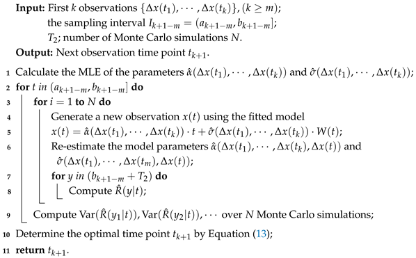
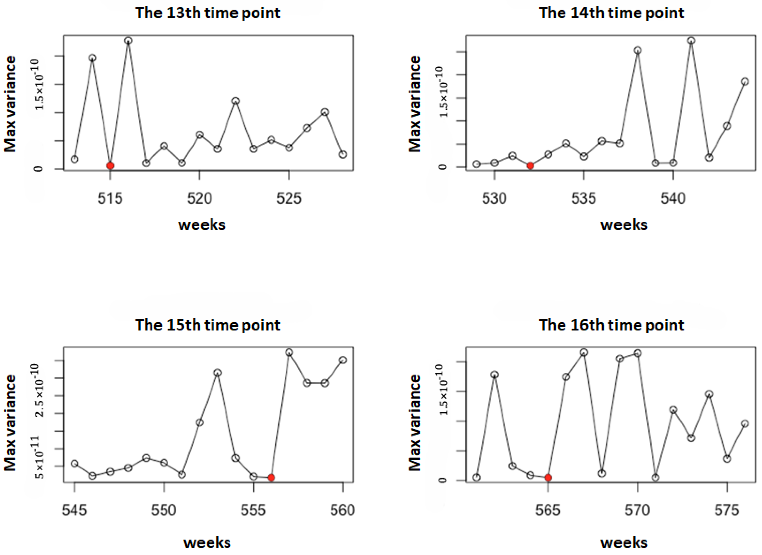
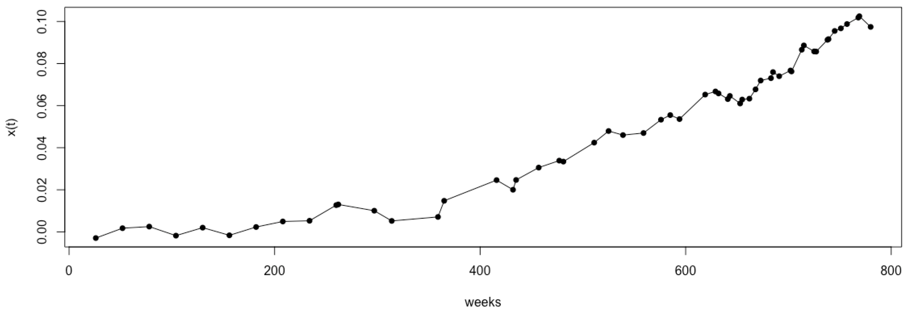
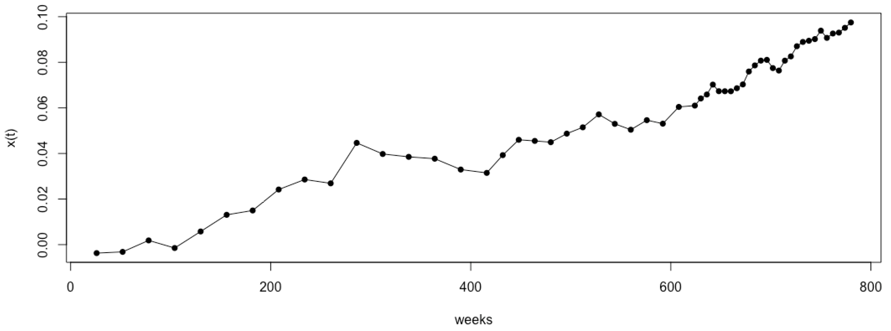
For illustration, taking Model 1 as an example, we set the number of Monte Carlo simulations to . Figure 1 shows the observation time points selected using the sequential-interval G-optimal method. The observation points selected by the G- and D-optimal methods for Model 1, along with their corresponding , are shown in Figure 2 and Figure 3, respectively. It can be observed that the sequential-interval G-optimal method sometimes selects time points toward the left of the interval and sometimes toward the right. However, overall, as time progresses, the selected points become increasingly dense.
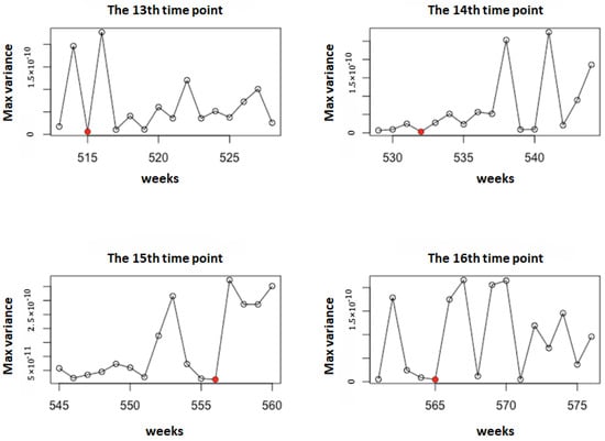
Figure 1.
The observation time points selected using the sequential-interval G-optimal method under Model 1 (). The red points represent the selected observation time points.

Figure 2.
The time points selected using sequential G-optimal interval sampling and the corresponding logarithm of the degradation value under Model 1 ().
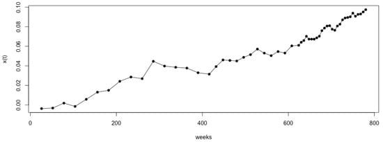
Figure 3.
The time points selected using sequential D-optimal interval sampling and the corresponding logarithm of the degradation value under Model 1 ().
We repeated the simulation 500 times for both the G-optimal sampling method and the D-optimal sampling method and computed the mean and the root mean squared error (RMSE) of the 500 predictions. The simulation results are shown in Table 3, Table 4 and Table 5, along with a comparison with the conditional C-optimal proposed by Wang.
Table 3.
Comparison of reliability prediction results for Model 1 ().
Table 4.
Comparison of reliability prediction results for Model 2 ().
Table 5.
Comparison of reliability prediction results for Model 3 ().
As can be seen from Table 3, when , the results obtained using the G-optimal and D-optimal sampling methods are both superior to those of Wang’s sampling method, as the means are closer to the true value and the RMSEs are smaller. Linear models are generally easier to estimate, which results in good model estimation performance under both D-optimal and G-optimal methods. The D-optimal method focuses on the precision of parameter estimation, while the G-optimal method emphasizes the accuracy of reliability prediction. In the case of linear models, accurate reliability prediction often implies accurate parameter estimation as well. Therefore, under linear degradation settings, the G-optimal method tends to yield better overall performance. Thus, the G-optimal method outperforms the D-optimal method. It is worth mentioning that Wang’s sampling method requires a larger and non-fixed number of sample points, with a median of 74. To investigate how changes in model parameters affect prediction error, we take Model 1 as an example and modify its parameters by multiplying the original values by , which corresponds to Scenario II. Since the drift coefficient, which governs the degradation rate, increases accordingly, we conduct simulation experiments to predict the reliability of satellite electronic devices with a designed lifespan of 8 years at time points of 8.5, 9, 9.5, and 10 years. Both the proposed G-optimal and D-optimal sampling methods are applied. The division of sampling intervals is the same as that in Model 3, as shown in Table 2. The simulation results are presented in Table 6, where Scenario I refers to the original Model 1. It can be seen that the impact of different model parameters on the prediction error is not significant.
Table 6.
Comparison of prediction errors under different parameter settings for Model 1 ().
In Table 4, when , it can be observed that, compared with Wang’s sampling method, the two optimal sampling methods proposed in this study did not consistently outperform. Except for the reliability prediction at year 15.5, the mean values of the G-optimal method are not closer to the true values compared to the D-optimal method. However, it is noteworthy that the RMSE of the G-optimal method is smaller, indicating reduced prediction variability. Nevertheless, as shown in the box plot on the left side of Figure 4, Wang’s sampling method requires more sample points. The median number of sample points required by Wang’s method is 74, whereas the proposed sequential-interval optimal sampling methods require a fixed number of 55 sample points. To further demonstrate the effectiveness of our proposed methods, we conducted two additional simulation studies for Model 1 and Model 2, respectively. The simulation results of our proposed G- and D-optimal methods with a fixed sample size of 74 (which is the median number of samples required by Wang’s sampling method) are presented in Table 7 and Table 8. The results demonstrate that, when using the same sample size as Wang’s sampling method, our proposed approaches yield consistently superior performance for both Model 1 and Model 2.
Figure 4.
Box plots of sample sizes for Model 2 and Model 3 using Wang’s sampling method.
Table 7.
Comparison of reliability prediction results for Model 1 () with 74 samples.
Table 8.
Comparison of reliability prediction results for Model 2 () with 74 samples.
As shown in Table 5, when , the D-optimal sampling method achieved consistently better results. Furthermore, as shown in the box plot on the right side of Figure 4, the number of sample points required by Wang’s sampling method exhibits significant fluctuations around the median, which is unfavorable for engineers in clearly planning observation schedules. In contrast, our sequential-interval optimal sampling method requires a fixed number of 48 sample points.
5. Conclusions
In this article, we consider a degradation model based on the Wiener process for the study of reliability prediction of long-lifespan electrical devices. The time-scale transformation in the model is , and we consider three cases: , , and . In practical reliability prediction problems, especially for high-reliability and long-lifespan electronic devices of satellites, engineers tend to obtain higher prediction accuracy using fewer degradation data, considering limitations in cost and data transmission capabilities. Therefore, we proposed more efficient sequential-interval G- and D-optimality approaches. The idea behind the G-optimal method is to minimize the worst-case prediction variance by minimizing the maximum variance, while the D-optimal method focuses on the precise estimation of the model parameters.
In the simulation study, using the reliability prediction of satellite MOSFETs as an example, we simulated degraded data to predict the reliability for the target years. Compared with the previous sampling method proposed by Wang, when the degradation model is a linear Wiener process, the method proposed in this article effectively improves prediction performance. Among them, the G-optimal design, which considers control of the worst-case prediction, yielded better and more stable results than the D-optimal method. When the degradation model is a nonlinear Wiener process, the G- or D-optimal sampling methods proposed in this paper achieve smaller RMSEs in most cases while maintaining comparable mean predictions. Additionally, the proposed method requires fewer samples, and the number of samples for sequential-interval optimal sampling can be determined in advance, which is more conducive to engineers planning the sampling process ahead of time.
There are several potential directions for future work. One key area for further investigation is incorporating the selection of sampling intervals into the optimization framework, thereby considering the optimization of interval settings and sampling strategies within each interval as a whole. This is particularly important when the degradation of electronic devices progresses slowly, in which case more effective methods are needed to predict their reliability. This remains a topic worthy of further research. Additionally, the composite process that combines shock-induced degradation and natural degradation often better reflects the actual degradation behavior of satellite electronic devices. The Wiener process is currently a widely adopted stochastic process in degradation analysis, optimal sampling methods that integrate discrete and continuous data should be developed for such processes. For example, , where denotes the overall degradation, represents the discrete degradation data, is the corresponding coefficient, and is the degradation model in our paper. This integrated model presents another promising avenue for future research. Exploring more efficient optimal sampling methods remains a challenging and significant direction for future work. With the advancement of technology, as data transmission between space and ground becomes more feasible, the development of a fully adaptive design is a highly promising direction for future exploration. Another important direction for future research is to investigate the sensitivity of the proposed sampling methods to model mis-specification. Since the Wiener process serves as an idealized assumption, it remains an open question as to whether the proposed sampling strategies maintain their effectiveness when applied to more complex degradation processes. Finally, when the degradation process of electronic components becomes more complex, the utilization of the Wiener process to describe the variation in the degradation amount and establish the corresponding degradation model may be limited. Future research can further explore more comprehensive multi-dimensional degradation modeling methods based on the approach proposed in this paper.
Author Contributions
Conceptualization, M.R. and Y.T.; Software, M.R. and X.L.; Investigation, Furi Guo; Writing—original draft, M.R.; Writing—review & editing, Y.T.; Supervision, Y.T.; Funding acquisition, Y.T. and F.G. All authors have read and agreed to the published version of the manuscript.
Funding
This work was supported by the National Natural Science Foundation of China (Grant no. 12131001) and the Natural Science Foundation of Shanxi Province (202303021221168).
Data Availability Statement
No new data were created or analyzed in this study. Data sharing is not applicable to this article.
Conflicts of Interest
The authors declare no conflicts of interest.
References
- Zhang, Z.; Si, X.; Hu, C.; Lei, Y. Degradation data analysis and remaining useful life estimation: A review on Wiener-process-based methods. Eur. J. Oper. Res. 2018, 10, 775–796. [Google Scholar] [CrossRef]
- Doksum, K.A.; Hbyland, A. Models for variable-stress accelerated life testing experiments based on Wiener processes and the inverse Gaussian distribution. Technometrics 1992, 34, 74–82. [Google Scholar] [CrossRef]
- Lu, C.J.; Meeker, W.O. Using degradation measures to estimate a time-to-failure distribution. Technometrics 1993, 35, 161–174. [Google Scholar] [CrossRef]
- Xu, Z.; Ji, Y.; Zhou, D. Real-time reliability prediction for a dynamic system based on the hidden degradation process identification. IEEE Trans. Reliab. 2008, 57, 230–242. [Google Scholar]
- Wang, X.; Balakrishnan, N.; Guo, B. Residual life estimation based on a generalized Wiener degradation process. Reliab. Eng. Syst. Saf. 2014, 124, 13–23. [Google Scholar] [CrossRef]
- Kang, W.; Tian, Y.; Xu, H.; Wang, D.; Zheng, H.; Zhang, M.; Mu, H. Reliability analysis based on the Wiener process integrated with historical degradation data. Qual. Reliab. Eng. Int. 2023, 39, 1376–1395. [Google Scholar] [CrossRef]
- Zheng, H.; Yang, J.; Zhao, Y. Reliability analysis of multi-stage degradation with stage-varying noises based on the nonlinear Wiener process. Appl. Math. Model. 2024, 125, 445–467. [Google Scholar] [CrossRef]
- Wang, G.; Li, X.; Fang, G.; He, Z.; Vining, G. Optimal design for reliability improvement experiments with a non-constant scale parameter. Qual. Technol. Quant. Manag. 2024, 21, 869–886. [Google Scholar] [CrossRef]
- Ardila, A.; Rodriguez, M.J.; Pelletier, G. Optimizing sampling location for water quality degradation monitoring in distribution systems: Assessing global representativeness and potential health risk. J. Environ. Manag. 2024, 365, 121505. [Google Scholar] [CrossRef] [PubMed]
- Li, X.; Song, K.; Shi, J. Degradation generation and prediction based on machine learning methods: A comparative study. Maint. Reliab./Eksploatacja i Niezawodność 2025, 27, 192168. [Google Scholar] [CrossRef]
- Wang, J.; Tian, Y. An adaptive reliability prediction method for the intelligent satellite power distribution system. IEEE Access 2018, 6, 58719–58727. [Google Scholar] [CrossRef]
- Wang, J.; Wang, D.; Tian, Y. Adaptive Bayesian prediction of reliability based on degradation process. Commun. Stat.-Simul. Comput. 2020, 51, 4788–4798. [Google Scholar] [CrossRef]
- Wang, X. Wiener processes with random effects for degradation data. J. Multivar. Anal. 2010, 101, 340–351. [Google Scholar] [CrossRef]
- Zhang, S.; Zhai, Q.; Li, Y. Degradation modeling and RUL prediction with Wiener process considering measurable and unobservable external impacts. Reliab. Eng. Syst. Saf. 2023, 231, 109021. [Google Scholar] [CrossRef]
- Yi, X.; Wang, Z.; Liu, S.; Tang, Q. Acceleration model considering multi-stress coupling effect and reliability modeling method based on nonlinear Wiener process. Qual. Reliab. Eng. Int. 2024, 40, 3055–3078. [Google Scholar] [CrossRef]
- Chen, W.; Hao, S. Condition-Based Operation and Maintenance Strategy for Load-Sharing Systems Based on Wiener Process. IEEE Trans. Reliab. 2025. [Google Scholar] [CrossRef]
- Zhang, L.; Wang, S.; Chen, X.; Guo, J.; Xu, L.; Ling, S.; Zhang, X. Failure analysis and reliability assessment of gold-plated fuzz buttons in elevated temperature. Microelectron. Reliab. 2025, 168, 115687. [Google Scholar] [CrossRef]
- Whitmore, G.A.; Schenkelberg, F. Modelling accelerated degradation data using Wiener diffusion with a time scale transformation. Lifetime Data Anal. 1997, 3, 27–45. [Google Scholar] [CrossRef]
- Fox, G.; Salazar, R.; Habib-Agahi, H.; Dubos, G.F. A satellite mortality study to support space systems lifetime prediction. In Proceedings of the 2013 IEEE Aerospace Conference, Big Sky, MT, USA, 2–9 March 2013; pp. 1–9. [Google Scholar]

Disclaimer/Publisher’s Note: The statements, opinions and data contained in all publications are solely those of the individual author(s) and contributor(s) and not of MDPI and/or the editor(s). MDPI and/or the editor(s) disclaim responsibility for any injury to people or property resulting from any ideas, methods, instructions or products referred to in the content. |
© 2025 by the authors. Licensee MDPI, Basel, Switzerland. This article is an open access article distributed under the terms and conditions of the Creative Commons Attribution (CC BY) license (https://creativecommons.org/licenses/by/4.0/).