Abstract
In the study of dynamic systems, bifurcation diagrams are a very popular graphical tool for studying stability and nonlinear changes in behavior. They are instrumental in analyzing the system’s response to parameter changes. These diagrams show the system’s various dynamic patterns and phase transitions by plotting the relationship between the system response and the parameters. This paper presents a computational algorithm for studying bifurcations in dynamic systems, especially for systems with chaotic behavior that depends on parameter changes. Depending on the type of system to be analyzed, the following two strategies for computing bifurcation diagrams are described: (i) detecting crossing points through the Poincaré plane and (ii) the identification of local maxima (or minima) in one of the system solutions. In addition, this paper presents a method for implementing parallel computation in MATLAB using the Parallel Computing Toolbox from MathWorks, which significantly reduces the computational time required to generate bifurcation diagrams. This work contributes to the study of dynamic systems by providing the reader with accessible tools for studying any dynamic system under established standards and reducing the computational time required for these types of studies by implementing these algorithms utilizing the multi-core processors found in modern computers.
Keywords:
bifurcation diagram; Feigenbaum diagram; dynamical systems; chaos; parallel computing; HPC MSC:
37C20; 65Y05; 65K05; 65E05
1. Introduction
For decades, scientists have been fascinated by the intricate interplay of order and chaos in dynamical systems. From the graceful orbits of celestial bodies to the irregular rhythms of heartbeats, dynamical systems permeate our understanding of nature.
Understanding chaos requires powerful analytical tools that can navigate the complexities of dynamic behavior. Small changes in initial conditions or system parameters—especially in systems exhibiting chaotic behavior—can significantly alter the system’s structure. Various methods, such as phase diagrams, Poincaré sections, and power spectrum analysis, can be employed to analyze these changes. Additionally, exploring the dynamics of a system across a range of parameters provides a broader understanding of its behavior. Bifurcation theory plays a crucial role in this exploration, as it focuses on transition models and helps identify instabilities within systems when parameters are varied [1,2].
A bifurcation represents a qualitative change in the solutions of differential equations as parameters are altered. Bifurcation diagrams graphically depict how a dynamic system’s behavior evolves with varying parameter values, illustrating transitions between stable states, limit cycles, and chaotic behavior. These diagrams apply to discrete and continuous systems, playing a crucial role in analyzing the dynamics of various differential equations and iterative maps [3,4]. Notably, the Feigenbaum diagram illustrates the sequence of period-doubling bifurcations as a path to chaos in discrete one-dimensional maps, such as the logistic or Hénon maps, revealing a universal proportion characterized by the Feigenbaum constant, which quantifies the diminishing intervals between successive bifurcations leading to chaos. While the bifurcation diagram is a general concept applicable to various systems, the Feigenbaum diagram focuses on discrete systems exhibiting this self-similar structure.
To construct bifurcation diagrams, the following two standard methods are employed: (i) analytical determination of critical change points in the system and (ii) numerical simulations using integration methods [5,6,7]. These approaches unveil intricate transition points, known as bifurcations, where ordered trajectories split into various behaviors. Such diagrams are widely applied across scientific fields, often generated through simulations to identify local maxima in time series for each studied bifurcation parameter. For instance, they analyze subharmonic resonance in rotor–ball bearing systems [8], evaluate ecological models of species interactions [9], and study the impact of immunotherapy on tumor growth [10]. Bifurcation diagrams are especially useful for exploring how coupling strength influences transitions between synchronized chaotic and unsynchronized periodic states in coupled systems. Research [11] has mapped system behavior across varying coupling strengths, identifying critical thresholds such as bistability onset and shifts between synchronized and unsynchronized states. These diagrams offer insights into the effects of coupling structures on dynamics and the relationship between feedback mechanisms and initial conditions.
The bifurcation diagrams used in the work described above are based on examining time series, identifying changes in the slope of one of the state variables, and viewing these inflection points as quantitative information about the system’s state. While this is one way to create a bifurcation diagram, there is no criterion for selecting the correct state variables to visualize the oscillator’s state transitions.
For example, the algorithms proposed in the recent MATLAB R2024b file sharing contributions [12,13,14] focus on the analysis of local maxima or intersection planes fixed in space. As mentioned in the descriptions of these algorithms, the placement of the intersection planes is influenced by the dynamics of the analyzed system.
In addition to these simulation-based methods, there are established bifurcation software tools such as AUTO [15], MatCont [16], and XPPAUT [17] that use numerical continuation methods to track equilibrium branches, periodic orbits, and bifurcation points. These packages usually require explicit model formulations and Jacobian matrices and are particularly suitable for analytically defined systems. In contrast, the algorithm proposed in this work is based on the detection of crossing events in the Poincaré plane directly from the simulated trajectories, making it applicable to both analytical and black-box models. Moreover, our method allows for the adaptive selection of the orientation of the Poincaré section—a feature not considered by standard tools or recent algorithmic contributions—and benefits from parallel computation to reduce processing time without compromising accuracy.
In this sense, the Poincaré plane is a technique that allows for the visualization of higher-dimensional flows in lower-dimensional spaces [18]. Taking a cross-section of a trajectory at regular intervals helps identify periodic trajectories, quasi-periodic behavior, and chaotic dynamics, becoming essential for understanding non-integrable Hamiltonian systems, stability theory, chaotic attractors, and as an auxiliary tool to calculate the fractal dimension of chaotic systems [19]. Henri Poincaré developed this concept during his work on the three-body problem, particularly in his prize-winning paper for the competition to celebrate the 60th birthday of King Oscar II of Sweden in 1889. With this work, he laid the foundations for what would later become modern chaos theory [20].
The computational resources needed to create these diagrams depend on various factors, including the accuracy of graphics visualizing transitions between chaotic and periodic points, the number of iterations required by the algorithms, and the arrangement of sections and intersection planes with different slopes.
We propose an algorithm that allows the user to study bifurcation dynamics by selecting the orientation of the Poincaré plane based on the system properties to be analyzed. Since computational efficiency is crucial in the analysis of complex dynamical systems, especially in the construction of bifurcation diagrams and the approximation of solutions to differential equations, our approach highlights the importance of optimizing both algorithm design and simulation performance through sequential and parallel programming or high-performance computing [21].
The main contributions of this work can be summarized as follows:
- Poincaré Plane Adaptation: The user-selected slope of the Poincaré plane is adapted to the system’s geometry, improving the accuracy of event detection;
- Transient Filtering: A mechanism to efficiently discard transient states and manage output storage, improving the robustness of system response to initial conditions;
- Modular Algorithm Design: Separation of the simulation, detection, and analysis phases, allowing flexible adaptation to different types of systems;
- Parallel Implementation: Use of the MATLAB construct parfor to significantly reduce processing time while maintaining numerical accuracy;
- Validation Through Case Studies: Application to well-known systems, including the Rössler and bidirectional Lorenz models, to demonstrate the effectiveness of the algorithm in solving complex bifurcation structures.
The sections of this article are as follows: The mathematical definition and the methodology for constructing a Poincaré plane, as well as the definition of a bifurcation diagram, are discussed in Section 2 and Section 3. The numerical results for two chaotic systems used as test oscillators (the Rössler system and a multiscroll generator) are presented in Section 4. Section 5 describes the algorithms and routines used to obtain the results shown. The results of the algorithms used are presented in Section 6, and the conclusions of the work are described at the end of the paper.
2. Mathematical Preliminaries
Following the ideas presented in [22,23], in this section, we present the formal mathematical description of trajectories within a continuous dynamical system, the concept of Poincaré planes, and bifurcation diagrams.
2.1. Poincaré Planes
The use of Poincaré sections to analyze periodic or chaotic behavior is well established in the study of nonlinear dynamical systems [24,25,26]. To construct a Poincaré plane, we should first consider a continuous dynamical system, expressed as follows:
where the state vector and the corresponding smooth vector field is denoted by . The system (1) induces a flow in the dimensional space [27]. For each initial condition , a trajectory is associated.
It is important to note that the system possesses a dissipation ball , such that . The maximal attractor is the largest invariant subset of that exhibits attraction. Also, the trajectory in the attractor is expressed as .
The Poincaré plane is an -dimensional surface, defined as follows:
where , with as coefficients of the hyperplane equation. To ensure that is perpendicular to the flow , the coefficients and slope are chosen to satisfy the transversality condition , and to ensure that the trajectory crosses recursively the Poincaré plane at the time instants , with . Generating crossing points , where with .
To achieve this, we focus on a set of points generated by the trajectory that crosses the Poincaré plane, defined as follows:
with , where satisfies the following:
Therefore, grows as , where # denotes the cardinality of the set.
We will then explore the case of three-dimensional benchmark systems, i.e., their solution belongs in . Therefore, the Poincaré plane will be as follows:
where the values of with will be set according to the slope needed and considering the characteristics of each system analyzed.
2.2. Bifurcation Diagrams
Now, to analyze transitions to chaos, we extend the autonomous system (1) by considering a variational parameter , as follows:
where governs the system’s dynamics. The parameter modulates qualitative changes in the attractor , which may evolve towards stable equilibria, periodic orbits, or chaotic attractors.
Since a bifurcation diagram visualizes the asymptotic behavior of trajectories as varies [24], we will use the Poincaré map from (3) to project intersections with onto a representative coordinate (e.g., ).
Then, one possible way to define the bifurcation diagram is as follows: Let be the bifurcation parameter that takes M equally spaced values from to , with step size , i.e., , for and . Then, the bifurcation diagram can be represented by the following geometric locus:
where, with a slight abuse of notation, is the matrix version of the set defined in (3), that is, it is a matrix where column j corresponds to , and row h corresponds to the h-th component of the state vector , i.e., . Note that the number of columns is not necessarily the same for all values of the parameter , which is why the superscript in is used as a label. Usually, the crossings obtained from transient states are discarded by considering .
3. Numerical Calculation of Poincaré Plane Crossing Events
We use the fourth-order Runge-Kutta (RK4) integration method to numerically solve the system of equations. Since numerical integration produces discrete trajectories rather than continuous ones, the exact location of a crossing event must be estimated. This section outlines the following three approaches for computing bifurcation diagrams from these discrete trajectories: two based on Poincaré crossings and one based on local maxima or minima.
3.1. Detecting a Poincaré Crossing
In the mathematical and analytical context, the crossing events with the Poincaré plane occur precisely at the instant the event is triggered, due to the continuous nature of the system’s trajectory. Given that the systems’ numerical solution corresponds to a discrete vector instead of a continuous one, the following assumptions must be considered.
Achieving a situation in which the numerical solution matches the crossing point of the plane at a specific trajectory point is challenging and typically requires an exceedingly small integration step, along with an infinite number of points in the solution. Thus, the crossing event must be calculated as illustrated in Figure 1, using a selection of points that marginally cross the plane in .
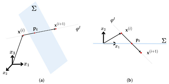
Figure 1.
Illustration of Poincaré Plane and crossing point in, (a) , (b) , considering numerical solutions of dynamical system.
In Figure 1a, the thin gray line represents the system’s trajectory in continuous time, the semi-transparent surface in light blue represents the Poincaré plane . The graph depicts three points in red, with the first on the left side of the image, called , representing the point of the system’s flow’s discrete numerical solution. Note that this point is located before the trajectory crosses the plane. Subsequently, on the right side of the plane, the point is also marked in red, which represents the next point in the discrete solution of the system’s flow, that is, given the integration step, there is no solution point between and . Now, the red point located on the plane, represented as , represents the crossing point of the continuous trajectory. This point needs to be estimated due to the discrete solution computed by RK4, indicating a crossing point between and for the reasons explained above, so it is necessary to calculate it using the following approximation.
To find the intersection point , we consider the vector that starts at the origin and heads toward and the vector that starts at and heads toward , both of which are marked with the black arrow lines. Note that the intersection determines a vector in the same direction as but of a smaller proportion. Given that and through the discussion presented after Equation (3), we can define the following:
with and that correspond to the proportion of the vector. Thus, an approximation and alternative form to describe Equation (4) with the discrete values obtained in the RK4 integration will be as follows:
Crossing in the Poincaré Plane
Many benchmark dynamical systems exhibiting strange attractors and parameter dependence typically oscillate around the origin. As a specific example, this algorithm will examine crossing events that occur in the plane described in Equation (5), with parameters set as and , positioning them within the plane. This analysis will replicate the calculations of the crossing events as established in the previous section. A projection onto the plane is presented in Figure 1b. In this case, the procedure to find the crossing event due to the numerical discrete points and will be the same as previously discussed, by the calculation of r given in Equation (9).
3.2. Map of the Local Maxima
Bifurcation diagrams can also be constructed using the local maxima (or minima) of the system’s flow based on a particular initial condition rather than relying on crossings through the Poincaré plane; in this sense, the transversality condition is no longer needed. This method facilitates the detection of bifurcations in trajectories that are not strictly constrained to a lower domain surface. To illustrate this approach, consider the sequence of point solutions , , and . A set of local maxima [28], can be identified as follows:
where depends on the state where the analysis will be conducted. In essence, we aim to pinpoint specific locations in space where the slope of the trajectory shifts from positive to negative. A similar procedure can be applied to identify local minima in Equation (10), using the criterion , where the slope of the trajectory transitions from negative to positive values. The coordinates of the points fulfilling the condition outlined in Equation (10) will be recorded as indicated in the map from Equation (3) for subsequent plotting.
4. Benchmark Systems
To study the algorithm, we will examine continuous dynamical systems in that exhibit chaotic behavior, gradual changes in the shape of the attractor, and period-doubling cascades that reflect various stable behaviors. For simplicity and without loss of generality in our notation, we will represent the states of these systems using the vector .
4.1. Rössler System
The first example of the bifurcation analysis of the algorithm will be the Rössler system [29], because it presents more continuous, gradual changes in attractor shape and rich parameter variation dynamics. The corresponding equations are described as follows:
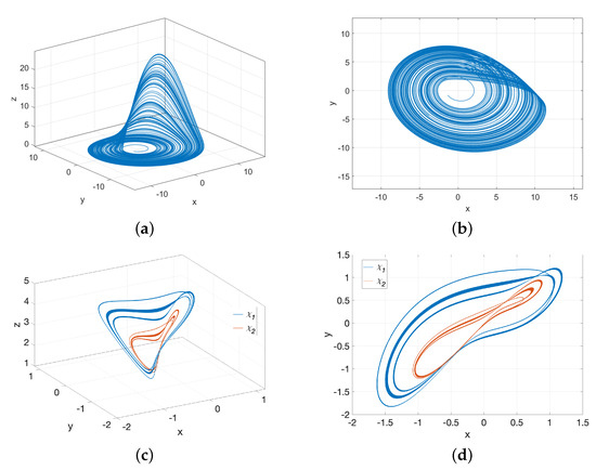
where are the states of the system and are the parameters to be analyzed. The system given in Equation (11) results in chaotic trajectories for and . Thus, we will study the bifurcation diagram for a range of values of the b parameter, maintaining fixed a and c for the different approaches described in Section 2. For illustrating purposes on the system’s behavior, Figure 2a depicts the chaotic attractor in . In contrast, Figure 2b shows a projection onto the plane. Considering the shape of the Rössler attractor and following the idea presented in [22], the slope of the plane Equation (5) was determined using the following coefficients ; and .
4.2. Bidirectional Coupled Lorenz Systems
While the algorithm is well suited for the Rössler system, calculating its bifurcation diagram may not be as computationally demanding. Therefore, we include a more complex example of the algorithm here. Specifically, we will consider a pair of bidirectionally coupled Lorenz systems, as presented in [11], whose interconnected dynamics require more detailed analysis. The system is represented by the following equations:
In this context, represents the state vector, and is the vector field that describes the dynamics of an isolated node. The dynamics are governed by the following equations:
where determines the system, are the state variables, are the system parameters, and is a scaling factor. We will utilize the common parameter values associated with chaotic behavior: , and we will set a scaling factor of .
The constants and in Equation (12) represent the coupling strengths between the systems. As outlined in [11], we will assume that is a negative constant (), while is a positive constant ().
The specific values of these coupling strengths lead to rich dynamic behaviors, including periodic, stable, and chaotic states. It is also crucial to note that the systems belong to . However, since the interconnection between them needs to be simulated simultaneously for both systems, we will be integrating them as a single system in . Figure 2c depicts the attractors (in blue line) and (in orange line) in for a coupling force of and . And Figure 2d shows a projection onto the plane.
5. Algorithms for Computing Bifurcation Diagrams
5.1. Architecture Specifications
The algorithms were implemented using MATLAB R2024b Update 4 (24.2.0.2833386) on a 64-bit (maca64) system. We will explore two approaches. Both are available for download as part of the Supplementary Materials. The first approach is a sequential algorithm that operates using iterative for-loops with the regular MATLAB worker assigned to the computer’s processor.
In this case, the algorithm’s processing time heavily depends on the number of divisions applied to the bifurcation parameter being studied and the length of the time vector, i.e., the number of time steps in the solution.
The second algorithm approach considers parfor-loops iterations distributed among parallel workers in a parallel pool. This approach is based on the Parallel Computing Toolbox of MathWorks, and the processing time also depends on the number of divisions implemented in the bifurcation parameter to be studied, the length of the simulated time, and the time step. However, as discussed later, it strongly depends on the number of cores of the running computer, as well as the number of selected workers by the parallel distribution.
5.2. Computation of a Sequential Bifurcation Diagram Using Iterative For-Loops
The initial method for computing bifurcation diagrams utilizes standard iterative for-loops without parallel distribution. This approach does not depend on toolboxes outside the base MATLAB platform. You can confirm this by using the command [fList, pList] = matlab.codetools.requiredFilesAndProducts(’run_main.m’), which will show the dependencies of the sequential algorithm. As a result, the output in pList.Name will reflect only the components included in the MATLAB distribution.
Sequential Algorithm Overview
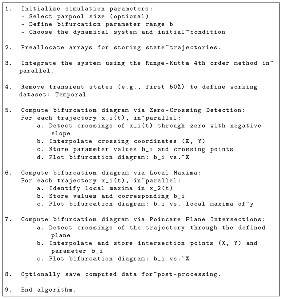
The algorithm systematically varies the bifurcation parameter and numerically solves the system for each value using the Runge–Kutta 4th order method (RK4). Typically, the time required to obtain the solution trajectories is longer than the processing time needed to detect the bifurcation points; however, this largely depends on the type of numerical integrator used. In the case of RK4, the algorithm implements four approximations for each solution point before evaluating the next point along the trajectory.
Once the system’s solution is obtained, we consider discarding at least 50– of the initial transient states due to the system’s complexity.
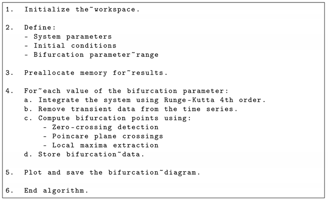
As a result, the bifurcation points are extracted using the methods mentioned earlier—Poincaré plane intersection, zero-crossing detection, and local maxima computation. The results are then stored and visualized in the final stage. Listing Section 5.2 presents the pseudo-code for this MATLAB implementation.
| Listing 1. Pseudo-code for iterative for-loop algorithm computing bifurcation diagram. |
 |
The main program is divided into five sub-files. As mentioned previously, the processing time depends on the number of divisions implemented in the bifurcation parameter to be studied, the length of the simulated time, and the time step. The following is a list describing the main file and each of the sub-files included:
- run_main.m: This is the main file for the algorithm. Users must select a bifurcation parameter within a specified range of values, ensuring that these values produce bounded trajectories in the integration method. The algorithm is limited to a fixed number of iterations, and a percentage of these iterations is later discarded as transient states, with the specific number determined by the user. The algorithm applies a designated function or subroutine for each integration method and bifurcation test. It is important to note that the algorithm does not exclude solutions even if the trajectories continue to grow over time. This can lead to inaccurate bifurcation diagrams with larger dimensions. Additionally, users can choose from various bifurcation detection algorithms (described in the subsequent sections) to analyze the system’s trajectories. If the process requires a substantial number of iterations to find a solution, the resulting data can be saved as a *.mat file to help manage the processing time of the algorithms.
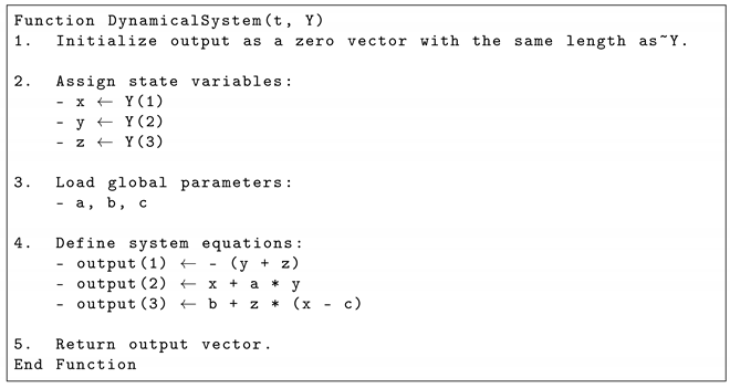
- DynamicalSystem.m: The equations for continuous dynamical systems must be included in this file. All bifurcation parameters considered in the study should be defined as global MATLAB variables to facilitate setting their values in the main file. The system should be configured to have one of its parameters vary within a specified range, as seen in the pseudo-code presented in Listing Section 5.2. The number of degrees of freedom for the system’s algorithm is . However, users may modify this with the size of the initial condition vector and select the proper systems with larger dimensionality. In this particular case, the Rössler system [29] is used as a benchmark example due to its chaotic behavior at certain parameter values.
- RungeKuttaBif.m: This routine implements the solution for dynamical systems using a numerical integration method with a fixed step size. We utilize the Runge–Kutta fourth-order method, which allows users to adjust the step size as needed. However, a step size of is generally sufficient for most benchmark systems. While MATLAB’s ode functions might be suitable depending on the complexity of the equations, we will not consider them in this work.
- Bif_ZeroCrossing.m: This routine determines and plots the bifurcation diagram of the system by analyzing the crossing events in the plane , as described in Equation (5). In this case, the slope parameters are set to and , as mentioned in Section 2.2. This method is applicable to systems where oscillates around the origin. Specifying a bifurcation parameter as part of the input global variables in the main file and a valid range of values is essential. The resolution and quality of the bifurcation diagrams depend on the initial conditions provided to the system.
- Bif_PoincarePlane.m: This routine calculates the bifurcation and plots the bifurcation diagram of the system considering the crossing events in the plane from Equation (5), with set by the user. This method is applicable to systems that oscillate throughout space, provided that the trajectory intersects the Poincaré plane via the coefficients .
- Bif_LocalMaxima.m: This routine calculates the local maxima of the system’s trajectory and generates the map given in Equation (10) with their location coordinates in space. If the dynamics of the system to be analyzed by the parameter variation is not completely known, this method will present a feasible alternative to plot their chaotic or periodic orbits. The program can be easily modified if the user needs the local minimum.
| Listing 2. Pseudo-code for DynamicalSystem.m function (Rössler system definition). |
 |
5.3. Parallelized Bifurcation Diagram Computation Using the Parallel Computing Toolbox
To improve computational efficiency, an alternative implementation was considered—distributing the iterations of the loop across multiple workers using MathWorks’ Parallel Computing Toolbox. This method allows computations to run simultaneously across several CPU cores, significantly reducing processing time.
Parallel Algorithm Overview
The core algorithm retains its iterative nature, but instead of a standard for-loop, a parallel parfor-loop distributes computations among the available/selected workers. The number of active workers is determined by the user’s configuration settings for the parallel pool, or they can specify the number of workers using the parpool function. In addition, for this program, we will use the same dependency facilities as in sequential computation, requiring only the MATLAB and Parallel Toolbox packages, as commented before in Section 5.2.
In this implementation, the algorithm is designed to take advantage of the capabilities of the Parallel Computing Toolbox by assessing the computer’s specifications and the number of cores in the processor to generate an optimal number of MATLAB workers. Due to the specifications of parfor, we cannot use global parameters in the code at this stage. As a result, the structure of this implementation differs slightly from that of the previous algorithm. Listing Section 5.3 presents the pseudo-code corresponding to this MATLAB code.
The main program is divided into three sub-files to calculate the bifurcation diagrams. The processing time depends on the number of divisions implemented in the bifurcation parameter to be studied, the length of the simulated time, and the time step. The following list describes the main file and each of the sub-files included:
- run_main_parfor.m: This is the main file of the algorithm and where the numerical integrations are processed. The user can select the number of parallel workers in this file using the Parallel Toolbox. This is adjusted with the command parpool(W), where W represents a valid number of cores available on the user’s machine. In our example, this line will be commented out so that the algorithm uses the maximum number of available cores. A key difference between a for-loop and a parfor-loop is that the latter cannot use global variables. Therefore, the system and its dimensions must be adjusted by selecting the initial conditions.
- Bif_ZeroCrossingPAR.m: This routine is similar to the sequential algorithm, which calculates the crossing events through for the selected systems and plots them. However, it distributes the calculations over the bifurcation parameter vector in the parallel pool.
- Bif_PoincarePlanePAR.m: Using a parfor-loop, this one calculates the bifurcation diagram of the system considering the crossing events in the plane from Equation (5), with set by the user.
- Bif_LocalMaximaPAR.m: Similarly, this routine calculates the local maxima of the system’s trajectory with a parfor-loop.
| Listing 3. Pseudo-code for the parallel bifurcation diagram algorithm using parfor. |
 |
6. Algorithm Functionality and Results
Given that the execution time of the algorithm used to generate the solution for the dynamical system heavily depends on the precision of the bifurcation parameter vector and the solution’s time step, it is generally recommended to run the program in two parts. At the end of the code, there is an option to save the system solutions using the “save” command. This allows the program to be executed in the following two phases: one for generating the numerical solutions of the system and the other for analyzing in-plane crossings and local maxima. Additionally, a visual aid in a progress bar has been implemented to help track progress and estimate execution times. The following flowchart (Figure 3) describes the subsequent process.
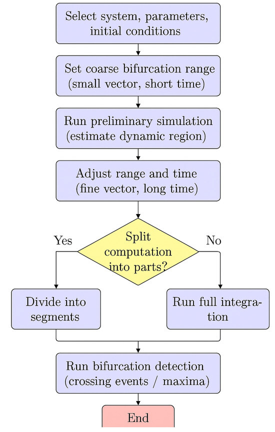
Figure 3.
Flowchart of bifurcation algorithm implementation process.
The algorithm’s implementation begins with the user selecting the dynamical system of interest and its associated parameters and initial conditions. Due to the event-based nature of the bifurcation detection procedure, a preliminary execution—referred to as a prerun—is recommended, using a reduced bifurcation vector and a limited number of integration steps. This step estimates the approximate location of the event-triggering conditions (e.g., Poincaré crossings) and informs the refinement of the bifurcation parameter range. Once the event locations are approximated, the bifurcation vector is adjusted to achieve the desired resolution. The algorithm is modularized into discrete parts to optimize computational efficiency and ensure robustness against long simulation times. This segmentation enables the storage and recovery of intermediate results, mitigating the risk of data loss during extended runs. Notably, the most computationally intensive component—the numerical integrator—can be executed and stored independently before the full bifurcation analysis. This allows for the reuse of the integrator output, streamlining the subsequent stages of the algorithm.
We now present the plotting of bifurcation diagrams resulting from the analysis of the two different systems.
6.1. Bifurcation Diagrams of the Rössler System
First, for the benchmark system example of the Rössler attractor given in Equation (11), a range of b is implemented for considering 500 steps, as presented in Listing Section 5.2. The time solution was calculated for with a time step of , removing the first transient states. Figure 4a shows the bifurcation diagram of the crossing events for a Poincaré plane located in the plane, as stated in Section 2. The values in which the system presents periodic or chaotic orbits can be easily identified here. Take, for instance, the values of , , , and , for which the system presents a 6-period orbit, chaotic behavior, a 2-period orbit, and a 1-period orbit, respectively, as the red dashed lines represent. This can be seen in greater detail in the individual projections in Figure 5. The dark blue line corresponds to the projection in space (a) and onto the plane (b). The Poincaré plane is depicted in a gray mesh or gray line, and the red asterisk represents the crossing events in the selected negative predefined slope (from top to bottom).
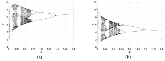
Figure 4.
(a) Bifurcation with the Poincaré plane; (b) Bifurcation with Zero crossing, both with Rössler system given in Equation (11).
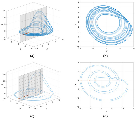
Figure 5.
Selection of Rössler system given in Equation (11). (a,b) . (c,d) .
6.2. Bifurcation Diagrams of the Bidirectional Lorenz System
The bifurcation diagram of the systems presented in Equation (12), calculated by the Poincaré plane located at , is presented in Figure 6 (a) for , and (b) for . We considered a variation in the coupling force parameter between with . The simulation considered a bifurcation vector size of 600 values and time steps, removing of the transient states. As mentioned in Section 4, the systems were simulated with an RK4 in . However, the bifurcation algorithm remained in . Both diagrams depict the intrinsic behavior of the systems for small variations in the coupling force.
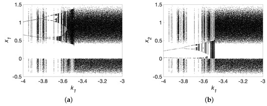
Figure 6.
Zero crossing of bidirectional Lorenz systems given in Equation (12) for a range of the coupling force and for (a) ; (b) .
7. CPU Performance Comparison Between Sequential and Parallel Algorithms
To evaluate the performance of the two versions of the algorithms, we used the cputime function in MATLAB, which measures the total CPU time utilized in seconds, following the recommendations provided by MathWorks for MATLAB scripts, specifically utilizing the cputime function to evaluate computational efficiency [30]. We define and as the execution time for the sequential and parallel algorithms, respectively. Our performance calculations focus solely on the numerical integration method and evaluate only the zero plane crossing detection, excluding waitbar commands and figure plots.
The solution of the bifurcation diagram is influenced by the system’s complexity, the number of time steps considered, and the precision or number of values used for the bifurcation parameter. We explore two general cases of the Rössler system, as described above. First, we use a vector with time step solution and a bifurcation parameter vector of varying size and precision. Specifically, we construct the vector using the function linspace, where for the Rössler bifurcation parameter b and . The vector size M was calculated from 20 to 300 precision divisions. Figure 7a illustrates the results of this experiment, showing that the sequential algorithm time, (depicted in blue), increases from for the bifurcation vector with 20 precision data to for a vector of 300 bifurcation values. In contrast, the parallel algorithm time (represented by the orange line) decreases, ranging from to for the same range of bifurcation vector sizes.
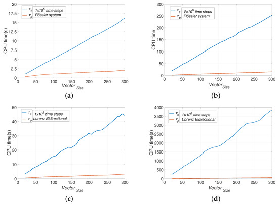
When we increased the time steps of the simulation to with the same bifurcation parameter vector size M from 20 to 300, we observed an increase in CPU execution times, as shown in Figure 7b. Here, the sequential algorithm time ranged from to , while the parallel case showed a time range of to .
Although the simulation times for the sequential case are not excessive, it is important to highlight that the Rössler system requires relatively less computational power for bifurcation analysis when compared to more complex systems, such as the Lorenz system. Hence, we conducted similar experiments using the same parameters for the bidirectional Lorenz systems. Figure 7c presents the results for the first case with solution times and bifurcation parameters ranging from 20 to 300 precision divisions. The sequential algorithm took approximately compared to for the parallel implementation. For the second case with solution times and the same range of bifurcation parameters, Figure 7d illustrates a significant difference in performance; the sequential algorithm took while the parallel algorithm completed in only . This shows a considerable reduction in execution time when using the parallel algorithms.
From the graphs shown in Figure 7, we can see that they all have a linear trend depending on the vector size containing the values for the bifurcation parameter; this allows us to determine the algorithm’s complexity. Since the computation time in our case only takes into account the numerical integration (the ) and the detection of the zero crossing (the ), it follows that the algorithm presented in this paper has a complexity of , which is confirmed by the above graphs.
Finally, to extend the validation of the proposed algorithms beyond classical chaotic systems, we implemented two well-known nonlinear oscillators in that exhibit periodic behavior. However, they transition from periodic to chaotic behavior under particular forcing conditions. The first system is the forced Duffing oscillator [31], described by the state-space representation, , where the parameters are set as , , , and . The second system is the forced Van der Pol oscillator [32], expressed as , with . These systems were selected for their ability to generate complex periodic responses and transitions toward chaotic regimes when varying the forcing amplitude . Additionally, the Rössler system in and the bidirectional coupled Lorenz system in were included to represent more complex and high-dimensional chaotic dynamics.
The computational performance comparison between the sequential and parallel implementations is summarized in Table 1. In this case, a bifurcation vector size of and time steps in the simulation and removing of the transient states, as these values resulted in a more suitable and visually appealing bifurcation diagram, as the graphs in Figure 4, Figure 6, and Figure 8 depict. The experiments confirm that, across all systems, the parallel implementation significantly outperforms the sequential version regarding CPU time reduction. Notably, the performance gain is particularly substantial in the bidirectional Lorenz system, where the execution time dropped from approximately 15,739.44 s to 84.62 s, achieving a speedup of 186×. In the lower-dimensional systems, such as the forced Duffing and forced Van der Pol oscillators, the observed speedup is approximately 20×, while for the Rössler system, the gain is around 15×. These results highlight that the parallel algorithm scales efficiently with both the system dimension and the resolution of the bifurcation parameter space, making it suitable for extensive bifurcation studies even in computationally demanding scenarios.

Table 1.
Performance comparison of sequential and parallel algorithms across different dynamical systems.
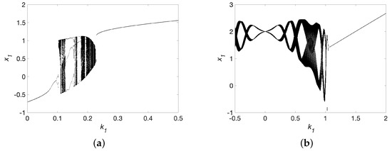
Figure 8.
Zero crossing of the (a) Force Duffing Oscillator for a range of the coupling force ; (b) Forced Van der Pol Oscillator for .
8. Concluding Remarks and Future Work
This paper presents a computational framework for bifurcation analysis in continuous dynamical systems that integrates three algorithmic strategies based on the rigorous formulation of discrete output vectors derived from numerical integration. By using Poincaré section crossings and local maxima, the method accurately identifies critical transitions in the system behavior. The inclusion of transient removal and adaptive storage further improves the detection of asymptotic dynamics, especially for systems with high sensitivity.
The effectiveness of the algorithm was validated using the Rössler and bidirectional Lorenz systems, successfully capturing complex bifurcation phenomena such as period doubling cascades and transitions between chaotic and periodic regimes. These results emphasize the robustness and adaptability of the system in solving complicated dynamic structures. Proof of this is the use of the proposed tools in the dynamical exploration of the Duffing forced system and the Van der Pol oscillator, two-dimensional dynamical systems (with periodic and chaotic behavior), where our algorithm efficiently computes the corresponding bifurcation diagrams.
A notable contribution is the integration of parallel computing, which significantly reduces computation time (as shown in Table 1). By isolating computationally intensive tasks—namely numerical integration and event detection—parallelization enables efficient scaling in terms of both simulation length and bifurcation resolution.
Despite its strengths, the approach has areas for improvement. The detection of events based on Poincaré crossings and local maxima can be affected by noise, possibly creating false bifurcation points or obscuring true transitions. Furthermore, selection of the appropriate Poincaré sections in higher-dimensional systems remains difficult and often requires adaptive or data-driven strategies to preserve transversality and recursion. The current framework also assumes smooth vector fields and does not directly consider hybrid or discontinuous systems where trajectory changes are abrupt. However, for piecewise systems, such as the one discussed in [33], a suitable choice of the slope of the Poincaré plane allows for an appropriate adaptation of the method, making our tool applicable in such a case.
Looking to the future, the algorithm’s applicability can be extended to a number of real-world domains. For example, in neuroscience, transitions between spiking and bursting dynamics can signal pathological states; in epidemiology, bifurcations can reveal tipping points in disease propagation; and in electrical engineering, oscillating circuits often show transitions between stable and unstable regimes.
Future research should address the integration of noise and time delays in system trajectories, benchmarking robustness and adaptation to non-smooth systems. The inclusion of an adaptive bifurcation parameter stepping strategy would enable dynamic refinement near critical points and coarsening in stable regions, thereby improving computational efficiency. Furthermore, the extension of the framework to higher-dimensional models, the implementation of adaptive step size control, and the use of machine learning for the automatic classification of dynamic regimes would further increase the benefits for research in the field of nonlinear dynamics.
Supplementary Materials
The following supporting information can be downloaded at: https://www.mdpi.com/article/10.3390/math13111818/s1, Two approaches.
Author Contributions
L.J.O.-G.: Conceptualization, Writing—Original Draft, Writing—Review and Editing, Methodology, Validation, Data Curation, Visualization, Project Administration. D.A.M.-G.: Writing—Review and Editing, Methodology, Validation. C.A.G.-G.: Writing—Review and Editing, Resources, Funding Acquisition. J.G.B.-R.: Writing—Review and Editing, Project Administration, Funding Acquisition. E.C.-C.: Visualization, Methodology, Validation. J.R.C.-G.: Review and Editing, Visualization, Methodology, Validation. J.P.-R.: Writing—Review and Editing, Project Administration, Validation. J.L.E.-M.: Writing—Review and Editing, Resources, Project Administration, Funding Acquisition. All authors have read and agreed to the published version of the manuscript.
Funding
This research was funded by the Potosino Council of Science and Technology (COPOCYT) with the Trust project 23871 of the 2023-01.
Data Availability Statement
The data used to support the findings of this study are available on the following website: https://github.com/luisjavier-ontanon/ParallelBifurcationDynamicalSystem (accessed on 19 May 2025).
Acknowledgments
L.J.O.-G. thanks the Potosino Council of Science and Technology (COPOCYT) for the support in Trust project 23871 of the 2023-01 Call. J.L.E.-M. thanks CONAHCYT for their support (CVU: 706850).
Conflicts of Interest
The authors declare no conflicts of interest.
References
- Arnold, V.I.; Wassermann, G.; Thomas, R. Catastrophe Theory; Springer: Berlin, Germany, 1986; Volume 3. [Google Scholar]
- Strogatz, S.H. Nonlinear Dynamics and Chaos: With Applications to Physics, Biology, Chemistry, and Engineering (Studies in Nonlinearity); Westview Press: Boulder, CO, USA, 2001; Volume 1. [Google Scholar]
- Baker, G.L.; Gollub, J.P. Chaotic Dynamics: An Introduction; Cambridge University Press: Cambridge, UK, 1996. [Google Scholar]
- Peitgen, H.O.; Jürgens, H.; Saupe, D.; Feigenbaum, M.J. Chaos and Fractals: New Frontiers of Science; Springer: New York, NY, USA, 2004; Volume 106. [Google Scholar]
- Luque, B.; Lacasa, L.; Ballesteros, F.J.; Robledo, A. Feigenbaum graphs: A complex network perspective of chaos. PLoS ONE 2011, 6, e22411. [Google Scholar] [CrossRef] [PubMed]
- Sprott, J.C. A proposed standard for the publication of new chaotic systems. Int. J. Bifurc. Chaos 2011, 21, 2391–2394. [Google Scholar] [CrossRef]
- Jafari, A.; Hussain, I.; Nazarimehr, F.; Golpayegani, S.M.R.H.; Jafari, S. A simple guide for plotting a proper bifurcation diagram. Int. J. Bifurc. Chaos 2021, 31, 2150011. [Google Scholar] [CrossRef]
- Hou, L.; Chen, Y.; Cao, Q.; Zhang, Z. Turning maneuver caused response in an aircraft rotor-ball bearing system. Nonlinear Dyn. 2015, 79, 229–240. [Google Scholar] [CrossRef]
- McAllister, A.; McCartney, M.; Glass, D.H. Food, fertilizer and Feigenbaum diagrams. Int. J. Math. Educ. Sci. Technol. 2024, 55, 171–183. [Google Scholar] [CrossRef]
- Sourailidis, D.; Volos, C.; Moysis, L.; Meletlidou, E.; Stouboulos, I. The study of square periodic perturbations as an immunotherapy process on a tumor growth chaotic model. Dynamics 2022, 2, 161–174. [Google Scholar] [CrossRef]
- Ontañón-García, L.J.; Cantón, I.C.; Ramirez, J.P. Dynamic behavior in a pair of Lorenz systems interacting via positive-negative coupling. Chaos Solitons Fractals 2021, 145, 110808. [Google Scholar] [CrossRef]
- Moysis, L.; Bifurcation Diagram for the Lorenz Chaotic System. MATLAB Central File Exchange. 2025. Available online: https://www.mathworks.com/matlabcentral/fileexchange/156752-bifurcation-diagram-for-the-lorenz-chaotic-system (accessed on 6 April 2025).
- Moysis, L.; Density-Colored Bifurcation Diagrams. MATLAB Central File Exchange. 2025. Available online: https://www.mathworks.com/matlabcentral/fileexchange/156757-density-colored-bifurcation-diagrams (accessed on 6 April 2025).
- Sylvestre-Baron, P.; Plotting Bifurcation Diagram. MATLAB Central File Exchange. 2025. Available online: https://www.mathworks.com/matlabcentral/fileexchange/72057-plotting-bifurcation-diagram (accessed on 6 April 2025).
- Doedel, E.; Oldeman, B. AUTO-07P: Continuation and Bifurcation Software for Ordinary Differential Equations. Concordia University. 2007. Available online: http://indy.cs.concordia.ca/auto/ (accessed on 6 April 2025).
- Dhooge, A.; Govaerts, W.; Kuznetsov, Y.A. MATCONT: A MATLAB package for numerical bifurcation analysis of ODEs. ACM Trans. Math. Softw. (TOMS) 2003, 29, 141–164. [Google Scholar] [CrossRef]
- Ermentrout, B. Simulating, Analyzing, and Animating Dynamical Systems: A Guide to XPPAUT for Researchers and Students; SIAM: Philadelphia, PA, USA, 2002. [Google Scholar]
- Poincaré, H. Sur le problème des trois corps et les équations de la dynamique. Acta Math. 1890, 13, A3–A270. [Google Scholar]
- Echenausía-Monroy, J.L.; Quezada-Tellez, L.A.; Gilardi-Velázquez, H.E.; Ruíz-Martínez, O.F.; Heras-Sánchez, M.d.C.; Lozano-Rizk, J.E.; Cuesta-García, J.R.; Márquez-Martínez, L.A.; Rivera-Rodríguez, R.; Pena Ramirez, J.; et al. Beyond Chaos in Fractional-Order Systems: Keen Insight in the Dynamic Effects. Fractal Fract. 2024, 9, 22. [Google Scholar] [CrossRef]
- Poincaré, H. Les Méthodes Nouvelles de la Mécanique Céleste; Gauthier-Villars et fils, Imprimeurs-Libraires: Paris, France, 1893; Volume 2. [Google Scholar]
- Garland, M.; Le Grand, S.; Nickolls, J.; Anderson, J.; Hardwick, J.; Morton, S.; Phillips, E.; Zhang, Y.; Volkov, V. Parallel computing experiences with CUDA. IEEE Micro 2008, 28, 13–27. [Google Scholar] [CrossRef]
- Ontanón-Garcia, L.J.; Campos-Cantón, E.; Femat, R.; Campos-Cantón, I.; Bonilla-Marín, M. Multivalued synchronization by Poincaré coupling. Commun. Nonlinear Sci. Numer. Simul. 2013, 18, 2761–2768. [Google Scholar] [CrossRef]
- Ontanón-Garcia, L.J.; Campos-Cantón, E. Discrete coupling and synchronization in the insulin release in the mathematical model of the β cells. Discret. Dyn. Nat. Soc. 2013, 1, 427050. [Google Scholar]
- Guckenheimer, J.; Holmes, P. Nonlinear Oscillations, Dynamical Systems, and Bifurcations of Vector Fields; Springer: New York, NY, USA, 1983. [Google Scholar]
- Strogatz, S.H. Nonlinear Dynamics and Chaos: With Applications to Physics, Biology, Chemistry, and Engineering; CRC Press: New York, NY, USA, 2018. [Google Scholar]
- Ott, E. Chaos in Dynamical Systems; Cambridge University Press: Cambridge, UK, 2002. [Google Scholar]
- Perko, L. Differential Equations and Dynamical Systems; Springer Science & Business Media: New York, NY, USA, 2013; Volume 7. [Google Scholar]
- Hancock, H. Theory of Maxima and Minima; Ginn: New York, NY, USA, 1917. [Google Scholar]
- Rössler, O.E. An equation for continuous chaos. Phys. Lett. A 1976, 57, 397–398. [Google Scholar] [CrossRef]
- MathWorks. Measure Performance of Your Program. 2024. Available online: https://www.mathworks.com/help/matlab/matlab_prog/measure-performance-of-your-program.html (accessed on 6 April 2025).
- Barba-Franco, J.; Gallegos, A.; Jaimes-Reátegui, R.; Muñoz-Maciel, J.; Pisarchik, A. Dynamics of coexisting rotating waves in unidirectional rings of bistable Duffing oscillators. Chaos Interdiscip. J. Nonlinear Sci. 2023, 33, 073126. [Google Scholar] [CrossRef] [PubMed]
- Salas, A.; Martínez H, L.J.; Ocampo R, D.L. Analytical and numerical study to a forced van der Pol oscillator. Math. Probl. Eng. 2022, 2022, 9736427. [Google Scholar] [CrossRef]
- Echenausía-Monroy, J.L.; Jafari, S.; Huerta-Cuéllar, G.; Gilardi-Velázquez, H. Predicting the emergence of multistability in a Monoparametric PWL system. Int. J. Bifurc. Chaos 2022, 32, 2250206. [Google Scholar] [CrossRef]
Disclaimer/Publisher’s Note: The statements, opinions and data contained in all publications are solely those of the individual author(s) and contributor(s) and not of MDPI and/or the editor(s). MDPI and/or the editor(s) disclaim responsibility for any injury to people or property resulting from any ideas, methods, instructions or products referred to in the content. |
© 2025 by the authors. Licensee MDPI, Basel, Switzerland. This article is an open access article distributed under the terms and conditions of the Creative Commons Attribution (CC BY) license (https://creativecommons.org/licenses/by/4.0/).