Rank-Based Family of Probability Laws for Testing Homogeneity of Variable Grouping

Abstract

In order to test within-group homogeneity for numerical or ordinal variable groupings, we have introduced a family of discrete probability distributions, related to the Gini mean difference, that we now study in a deeper way. A member of such a family is the law of a statistic that operates on the ranks of the values of the random variables by considering the sums of the inter-subgroups ranks of the variable grouping. Being so, a law of the family depends on several parameters such as the cardinal of the group of variables, the number of subgroups of the grouping of variables, and the cardinals of the subgroups of the grouping. The exact distribution of a law of the family faces computational challenges even for moderate values of the cardinal of the whole set of variables. Motivated by this challenge, we show that an asymptotic result allowing approximate quantile values is not possible based on the hypothesis observed in particular cases. Consequently, we propose two methodologies to deal with finite approximations for large values of the parameters. We address, in some particular cases, the quality of the distributional approximation provided by a possible finite approximation. With the purpose of illustrating the usefulness of the grouping laws, we present an application to an example of within-group homogeneity grouping analysis to a grouping originated from a clustering technique applied to cocoa breeding experiment data. The analysis brings to light the homogeneity of production output variables in one specific type of soil.

1. Introduction

In this work, taking as a starting point a statistic introduced in [1], we formally define and study a family of discrete finite probability laws that are useful to test the within-group homogeneity of groupings—or clusters—of observations for a finite set of random variables.

We call an element of this family of probability laws a grouping distribution. A grouping distribution, of the family we are interested in, is related to the Gini’s mean difference (for information on this statistic, see [2,3,4,5]). It has also some affinity with the distribution used in the Kruskal–Wallis test (see [6]) but, while this test compares ranks across multiple groups but focuses on the between-group variance of ranks, the grouping distribution focuses on the within-group dispersion.

The most well known homogeneity test is based on the Chi-square statistic and is applied to samples of numerical variables to determine if the samples originate from the same distribution. In this sense, homogeneity is an intergroup property, that is, the groups are homogeneous to one another, or not. In the same vein, the work [7] studies a family of nonparametric tests to decide if two independent samples have a common distribution with the same density; the tests rest on a family of distances between densities. In this work, we consider “homogeneity” in the sense of the homogeneity of elements within the groups; the principle is that, using some criteria, we first partition the data in groups, and then we test if the partition criteria give rise to groups which are homogeneous by themselves, or not.

In our approach, a grouping distribution is applied to a finite set of ranks of observations of random variables and so, as a consequence, a fruitful study of the grouping statistic law seems to rely heavily on combinatorics. To the best of our knowledge, the distribution of a random variable with the grouping probability law can only be determined with computational help due to the large number of events.

Among the tools available for the study of probability laws, the transform methods such as Laplace, Fourier or z-transform, for instance, are usually effective. The study of the Fourier transform by means of signal theory does not appear to be useful since the patterns observed in the graphical representations of the Fourier transforms of the laws result from an artifact—the French battement—resulting from the interference of trigonometric waves with frequencies close to one another.

The idea of considering semigroups generated either by the values taken by the distributions of the probabilities of the values can be motivated by the description of sums of independent random variables having a common grouping law. We will deal with this idea in another article.

Let us briefly describe the contents and main contributions of this work.

• In Section 2, we define the family of grouping distributions—which, in our opinion, should be denominated Mexia distributions, honoring the statistician extraordinaire João Tiago Mexia who proposed them for the first time—we detail some properties of the family and present tables of quantiles of the grouping distributions for moderate values of parameters computed from the full discrete distribution, and we state some remarks that highlight the motivation for the problems studied in the following.
• In Section 3, we present some results on moment generating functions that may have an independent interest, namely, Theorem 3, showing, under some general hypothesis, that the Kolmogorov distance between probability distributions is bounded by the $L^1$ distance between the correspondent moment generating functions. We prove a negative asymptotic result based on observed properties of some fully computable grouping distributions and we propose two methodologies to build approximate laws for grouping distributions with large parameter values; these methodologies may be considered implementation open problems due to technical difficulties.
• In Section 4, we present an application of a grouping distribution to assess the within-group homogeneity of clusters of observations from a cocoa breeding experiment.
  The clusters are obtained by the well-known KMeans clustering technique applied to the whole set of values of the variables. We show that the use of the grouping distribution allows to recover some important features of the observations, namely, the homogeneity of production variables in one type of soil that other statistical methods—such as ANOVA—do not bring to light.

The figures and the computations are performed using Wolfram’s Mathematica ™.

2. The Definition of the Grouping Probability Law

In this section, we define—in a constructive way, that is, by giving the values and the algorithm to obtain the correspondent probabilities—the family of the grouping probability laws.

Definition 1

(The family of grouping probability laws). The grouping test statistic law—denoted by $\mathcal{G}(N,p,n_1,\dots ,n_p)$—is the probability law defined by the following:

1. 

The set of integers $\mathcal{S}=\{1,2,\dots ,N\}$;

2. 

The set ${\mathit{S}}_p$ of all partitions of $\mathcal{S}$ in p subsets $\{{\mathcal{S}}_1,\dots ,{\mathcal{S}}_p\}$ such that

$$\#{\mathcal{S}}_k=n_k,k=1,\dots ,p and n_1+\dots +n_p=N.$$

3. 

The values of the following function $Q_{\mathcal{G}}$, defined on ${\mathit{S}}_p$:

$$Q_{\mathcal{G}}({\mathcal{S}}_1,\dots ,{\mathcal{S}}_p)=\sum _{k=1}^p\sum _{i,j\in {\mathcal{S}}_k}\left|i-j\right|,\{{\mathcal{S}}_1,\dots ,{\mathcal{S}}_p\}\in {\mathit{S}}_p,$$

(1)

from which we can obtain the corresponding frequencies of those values.

Let us detail some important observations about this family of probability laws. Firstly, it is a useful family for a statistical diagnostic of lack of homogeneity in groups; an example of such a statistical application is presented in Section 4. Secondly, the actual computation of values and respective frequencies is a challenge even for moderate values of N, say, for example $N=27$; in fact, for $N=27$, $p=2$, $n_1=15$, and $n_2=12$, we have that $\#{\mathit{S}}_2$ = 17,383,860, a number that can bring a computational challenge. Let us look first at some aspects of the possible statistical applications.

2.1. Statistical Relevance of Grouping Distributions

We first observe an elementary fact that is relevant for the control of any algorithm computing the law of a grouping distribution in the sense that it allows to estimate some of the worst case scenarios.

Remark 1

(The largest value for the partitions). Since the number of ways of depositing N distinct objects into p distinct bins, with $n_1$ objects in the first bin, $n_2$ objects in the second bin, and so on, is given by the multinomial coefficient and since $n_1+\cdots +n_p=N$, we obtain that

$$\#{\mathit{S}}_p={\displaystyle \frac{N!}{n_1!\cdots n_p!}}.$$

(2)

and so $\#{\mathit{S}}_p$ takes one of its largest values whenever we have

$$n_k\approx {\displaystyle \frac{N}{p}},k=1,\dots ,p.$$

See Appendix A.4 for an idea of a proof.

Remark 2

(Notation and example). We write $X⌢\mathcal{G}(N,p,n_1,\dots ,n_p)$ to denote a random variable X that follows the law $\mathcal{G}(N,p,n_1,\dots ,n_p)$, that is, X takes the values taken by $Q_{\mathcal{G}}$, defined in Formula (1), with the corresponding frequencies or probabilities. Let us consider the law $\mathcal{G}(9,2,4,5)$. The number of possible partitions is equal, according to Formula (2), to 126. But the set of values taken by $Q_{\mathcal{G}(9,2,4,5)}$ has only 16 different values; these values, together with the corresponding probabilities or frequencies of occurrence, are displayed in

Table 1. Values and corresponding probabilities for $\mathcal{G}(9,2,4,5)$.

$(60,\frac{1}{63})$	$(74,\frac{1}{63})$	$(84,\frac{2}{63})$	$(90,\frac{1}{21})$	$(92,\frac{2}{63})$	$(94,\frac{1}{63})$	$(100,\frac{1}{14})$	$(102,\frac{2}{63})$
$(106,\frac{2}{21})$	$(108,\frac{10}{63})$	$(110,\frac{1}{21})$	$(112,\frac{5}{126})$	$(114,\frac{10}{63})$	$(116,\frac{1}{6})$	$(118,\frac{4}{63})$	$(120,\frac{1}{126})$

.

Neither the values nor the frequencies of occurrence of these values, in Table 1, convey a discernible pattern of regularities allowing for an a priori description of values and corresponding probabilities for the law $\mathcal{G}(9,2,4,5)$. The quest for regularities allowing such an a priori description is a very interesting theme of research not considered in this work.

Remark 3

(On the statistical use of the grouping law). Given a collection of N random variables with completely ordered values—for instance, numerical random variables—it may be advisable to consider the partition of the N random variables in p groups of these random variables; the reason may be multifold: common origins, common data collecting structure, common structural characteristics, or even as a result of some clustering process. In order to test the statistical significance of the within-group homogeneity of the grouping, we consider, for each group, the global ranks of each of the variables of the group; such an attribution of ranks is possible since the variables have completely ordered values. This grouping procedure defines an initial family $\{{\mathcal{S}}_1,\dots ,{\mathcal{S}}_p\}$ of subsets of $\mathcal{S}=\{1,2,\dots ,N\}$—such that $\#S_i=n_i$—for which the function $Q_{\mathcal{G}}({\mathcal{S}}_1,\dots ,{\mathcal{S}}_p)$ has a determined value. The grouping will have statistical significance if the value of $Q_{\mathcal{G}}({\mathcal{S}}_1,\dots ,{\mathcal{S}}_p)$ is small enough with respect to all the other possible values of the function $Q_{\mathcal{G}}$ taken on all possible partitions of $\mathcal{S}=\{1,2,\dots ,N\}$ in different p subsets $\{{\mathcal{S}}_1^{\prime },\dots ,{\mathcal{S}}_p^{\prime }\}$ such that $\#S_i^{\prime }=\#S_i=n_i$. Once we have the law $\mathcal{G}(N,p,n_1,\dots ,n_p)$ we can define lower quantiles of this law and perform the adequate statistical test.

Let us look at two tables of quantiles $q_{\alpha }$—

Table 2. Quantiles $q_{\alpha }=q_{0.05}$ and $q_{\beta }=q_{0.1}$ for groupings in sets having as elements $N=14,15,\dots ,19$.

14	${\mathit{q}}_{\mathit{\alpha }},{\mathit{q}}_{\mathit{\beta }}$	15	${\mathit{q}}_{\mathit{\alpha }},{\mathit{q}}_{\mathit{\beta }}$	16	${\mathit{q}}_{\mathit{\alpha }},{\mathit{q}}_{\mathit{\beta }}$	17	${\mathit{q}}_{\mathit{\alpha }},{\mathit{q}}_{\mathit{\beta }}$	18	${\mathit{q}}_{\mathit{\alpha }},{\mathit{q}}_{\mathit{\beta }}$	19	${\mathit{q}}_{\mathit{\alpha }},{\mathit{q}}_{\mathit{\beta }}$
(2,12)	598	(2,13)	778	(2,14)	964	(2,15)	1178	(2,16)	1422	(2,17)	1698
$″$	618	$″$	778	$″$	984	$″$	1200	$″$	1450	$″$	1728
(3,11)	512	(3,12)	670	(3,13)	832	(3,14)	1022	(3,15)	1260	(3,16)	1512
$″$	528	$″$	678	$″$	852	$″$	1046	$″$	1284	$″$	1540
(4,10)	446	(4,11)	580	(4,12)	724	(4,13)	910	(4,14)	1110	(4,15)	1350
$″$	466	$″$	598	$″$	752	$″$	934	$″$	1146	$″$	1380
(5,10)	400	(5,10)	514	(5,11)	652	(5,12)	814	(5,13)	1004	(5,14)	1220
$″$	416	$″$	536	$″$	676	$″$	842	$″$	1036	$″$	1256
(6,8)	374	(6,9)	476	(6,10)	600	(6,11)	750	(6,12)	922	(6,13)	1118
$″$	394	$″$	502	$″$	628	$″$	780	$″$	954	$″$	1156
(7,7)	364	(7,8)	456	(7,9)	568	(7,10)	706	(7,11)	864	(7,12)	1044
$″$	384	$″$	482	$″$	596	$″$	734	$″$	896	$″$	1084
–	–	–	–	(8,8)	560	(8,9)	684	(8,10)	830	(8,11)	998
–	–	–	–	$″$	588	$″$	714	$″$	862	$″$	1036
–	–	–	–	–	–	–	–	(9,9)	816	(9,10)	974
–	–	–	–	–	–	–	–	$″$	852	$″$	1012

and

Table 3. Quantiles $q_{\alpha }=q_{0.05}$ and $q_{\beta }=q_{0.1}$ for groupings in sets having as elements $N=8,9,\dots ,13$.

8	${\mathit{q}}_{\mathit{\alpha }},{\mathit{q}}_{\mathit{\beta }}$	9	${\mathit{q}}_{\mathit{\alpha }},{\mathit{q}}_{\mathit{\beta }}$	10	${\mathit{q}}_{\mathit{\alpha }},{\mathit{q}}_{\mathit{\beta }}$	11	${\mathit{q}}_{\mathit{\alpha }},{\mathit{q}}_{\mathit{\beta }}$	12	${\mathit{q}}_{\mathit{\alpha }},{\mathit{q}}_{\mathit{\beta }}$	13	${\mathit{q}}_{\mathit{\alpha }},{\mathit{q}}_{\mathit{\beta }}$
(2,6)	72	(2,7)	114	(2,8)	186	(2,9)	260	(2,10)	352	(2,11)	464
$″$	84	$″$	128	$″$	186	$″$	274	$″$	368	$″$	482
(3,5)	60	(3,6)	102	(3,7)	148	(3,8)	208	(3,9)	296	(3,10)	392
$″$	68	$″$	102	$″$	156	$″$	222	$″$	304	$″$	410
(4,4)	52	(4,5)	84	(4,6)	126	(4,7)	180	(4,8)	248	(4,9)	332
$″$	60	$″$	90	$″$	130	$″$	188	$″$	264	$″$	356
–	–	–	–	(5,5)	120	(5,6)	160	(5,7)	228	(5,8)	304
–	–	–	–	$″$	128	$″$	182	$″$	240	$″$	320
–	–	–	–	–	–	–	–	(6,6)	216	(6,7)	286
–	–	–	–	–	–	–	–	$″$	236	$″$	302

—of the grouping distributions $\mathcal{G}(N,2,r,N-r)$, for $N=8,\dots ,19$ and $r=2,\dots ,N-2$, observing that due to the fact that there are only two subgroups, $p=2$, there is a symmetry, allowing us to reduce the number of cases presented. In this case, a statistical analysis focuses on testing the homogeneity of $p=2$ groups.

With the quantile Table 2 and Table 3, the statistical test may be performed in the following way. Consider a set of values—corresponding to the observation of random variables—a set with a number of elements between 8 and 19, let us say, for example, $N=13$ elements; this set can be decomposed into two groups corresponding to $(n_1,n_2)$ such that $n_1+n_2=N$ as follows: (2,11), (3,10), (4,9), (5,8) and (6,7). Suppose we have to test the homogeneity of a decomposition of the set of 13 values in two groups, for example, the decomposition (4,9), that is, in one subgroup with 4 values and the other subgroup with 9 values. In Table 3, we obtain the quantiles $q_{0.05}$ = 332 and $q_{0.1}$ = 356. We then order the 13 values and we consider the ranks of these values. Considering the subset of ranks ${\mathcal{S}}_1$ corresponding to the subgroup with 4 values and the subset of ranks ${\mathcal{S}}_2$ of the subgroup with 9 values, we can compute the value of the statistic $Q_{\mathcal{G}}({\mathcal{S}}_1,{\mathcal{S}}_2)$ defined in Formula (1) and compare it with a quantile, say $q_{0.05}$ or $q_{0.1}$, for some instances. Since the more significant one is the within-group homogeneity of the grouping, the lesser one is the value of the statistic $Q_{\mathcal{G}}({\mathcal{S}}_1,{\mathcal{S}}_2)$; an observation of a statistic value smaller that one of the chosen quantiles will provide indication of the within-group homogeneity.

2.2. Computational Issues for the Groupings Statistic Family

We first observe that the number of ways to partition a set of N objects into p non-empty subsets without the restriction of having a determined number of elements in each subset as in Definition 1 and Remark 1—a number denominated Stirling number of the second kind, or Stirling partition number—is given by

$$S(N,p)={\displaystyle \frac{1}{p!}}\sum _{i=0}^p{(-1)}^{p-i}\left({\displaystyle \genfrac{}{}{0pt}{}{p}{i}}\right)i^N=\sum _{i=0}^p{\displaystyle \frac{{(-1)}^{p-i}{i}^N}{(p-i)!i!}}$$

(3)

for $N\ge 1$ and $p\le N$ (see [8], p. 258) for substantial information on this subject). It is clear that for $N\ge 2$, we have $S(N,2)=2^{N-1}-1$, and so we have exponential growth, with N, of the number of evaluations, for $({\mathcal{S}}_1,{\mathcal{S}}_2)$, of the statistic $Q_{\mathcal{G}}({\mathcal{S}}_1,{\mathcal{S}}_2)$ for the family of probability laws $\mathcal{G}(N,2,r,N-r)$ when r varies.

Moreover, summing $S(N,p)$ in Formula (3), over all possible p, we obtain the total number of partitions of N, that is, the Bell number, a number that grows super exponentially (see [8], pp. 374, 493, 603).

This observation suggest two approaches. A first approach is to have at our disposal a set of asymptotic results allowing to approach the laws $\mathcal{G}(N,p,n_1,\dots ,n_p)$, for large values of N, more easily computable distributions. We present a negative result in Section 3 that leads to the proposal of two methodologies to obtain approximations for the grouping laws for large parameter values. A second approach consists of studying the structure of the distributions $\mathcal{G}(N,p,n_1,\dots ,n_p)$ in order to find regularities allowing for amenable computations; we defer to a posterior publication for some preliminary results with this approach, where we use elementary numerical semigroup facts to study convolutions of grouping laws.

3. On an Asymptotic Result for Some Grouping Distributions

Suppose that we have a random variable X with $\mathcal{G}(N,p,n_1,\dots ,n_p)$ grouping distribution taking the values ${\alpha }_i$ with probabilities $p_i$ with $i=1,\dots ,m$. We know that the higher numbers of different configurations of groupings occur when $n_j\approx N/p$ for all $j=1,\dots ,p$. In this case, it is to be expected that both m, that is, the number of different values taken by X—denoted by ${\alpha }_i$—and, simultaneously, these values ${\alpha }_i$ taken by X, will all be large, while, concurrently, the values of the probabilities $p_i$ such that $p_1=\mathbb{P}[X={\alpha }_i]$ will be uniformly small. In the case of N and p being simultaneously large, the computational burden of computing the discrete finite valued distribution is excessive, and so it would be useful to have an asymptotic result for the X grouping distribution.

Let us firstly detail some of the challenges we face in the quest for an asymptotic result. We take as an example a random variable X with the grouping distribution $\mathcal{G}(23,2,11,12)$; we first consider the values taken by X and the respective probabilities of occurrence and, from those, we obtain the probability law of the corresponding standardized random variable Y from which we can derive the empirical distribution. The PDF of the empirical distribution of Y is depicted in blue color in Figure 1.

We also fitted the discrete data $(x,ln\left({\mathrm{pdf}}_Y\left(x\right)\right)$ of the logarithm of ${\mathrm{pdf}}_Y\left(x\right)$, the PDF function of Y, by a function of the form $f\left(x\right)=a+b(x-c)+d{(x-e)}^2$, thus obtaining, upon the exponentiation of $f\left(x\right)$ and the normalization of $e^{f\left(x\right)}$, a fitting by a normally distributed random variable of the standardized data of X. The PDF of the normal distribution fitting the PDF of the empirical distribution of Y is depicted in red color also in Figure 1. We observe that the PDF in blue is more akin to a trajectory of a stochastic process having as a mean the PDF in red. The lower irregularity in the left tail of the blue PDF is why, in our perspective, we can only expect an asymptotic normality result that can give acceptable results only for the lower quantiles of the law $\mathcal{G}(N,p,n_1,\dots ,n_p)$.

3.1. Some Auxiliary Results on Moment Generating Functions

We first prove an auxiliary result—Theorem 3 ahead—that shows that if we have some control over the behavior of a sequence of moment generating functions, then we also have control over the sequence of the correspondent distribution functions. For that purpose, in the sequel, we consider the following setting of main hypothesis.

We have probability laws $\mu$ and ${\left({\nu }_n\right)}_{n\ge 1}$ with respective densities $f_{\mu }\left(x\right)$ and ${\left(f_{{\nu }_n}\left(x\right)\right)}_{n\ge 1}$ and the correspondent moment generating functions (MGFs) defined by

$${\mathcal{M}}_{\mu }\left(t\right)={\int }_{-\infty }^{\infty }{e}^{tx}{f}_{\mu }\left(x\right)dx,{\mathcal{M}}_{{\nu }_n}\left(t\right)={\int }_{-\infty }^{\infty }{e}^{tx}{f}_{{\nu }_n}\left(x\right)dx.$$

(4)

Let us suppose that the following holds:

• The densities $f_{\mu }\left(x\right)$ and $f_{{\nu }_n}\left(x\right)$ have exponential decay that is

  $$\exists {\lambda }_1,{\lambda }_2>0,\forall n\ge 1,|f_{\mu }\left(x\right)|\le {\lambda }_1{e}^{-{\lambda }_2\left|x\right|},\left|f_{{\nu }_n}\left(x\right)\right|\le {\lambda }_1{e}^{-{\lambda }_2\left|x\right|}.$$
  This is equivalent to the fact that the interior of the sets ${\mathit{D}}_{\mu }:=\{t\in \mathbb{R}:{\mathcal{M}}_{\mu }\left(t\right)<+\infty \}$ and ${\mathit{D}}_{{\nu }_n}:=\{t\in \mathbb{R}:{\mathcal{M}}_{{\nu }_n}\left(t\right)<+\infty \}$—that is, respectively, $\mathring{{\mathit{D}}_{\mu }}$ and $\mathring{{\mathit{D}}_{{\nu }_n}}$—are non-empty sets (see Proposition 5.1 in [9]). The sets ${\mathit{D}}_{\mu }$ and ${\mathit{D}}_{\nu }$ are, in fact, intervals.
• Also as a consequence, we have that ${\mathcal{M}}_{\mu }(\sigma +i\omega )$ and ${\mathcal{M}}_{{\nu }_n}(\sigma +i\omega )$ are holomorphic (analytic) in a strip of the complex plane defined by $\sigma \in \mathring{{\mathit{D}}_{\mu }}\cap \mathring{{\mathit{D}}_{{\nu }_n}}$ (see Proposition 5.3 in [9]).
• For every $\sigma +i\omega$ in the complex plane strip defined by $\sigma \in \mathring{{\mathit{D}}_{\mu }}\cap \mathring{{\mathit{D}}_{{\nu }_n}}$, we have that

  $$\underset{n\to +\infty }{lim}{\mathcal{M}}_{{\nu }_n}(\sigma +i\omega )={\mathcal{M}}_{\mu }(\sigma +i\omega ).$$
• There exists an integrable function G in the variable $\omega$ such that, for every $\sigma +i\omega$ in the complex plane strip defined by $\sigma \in \mathring{{\mathit{D}}_{\mu }}\cap \mathring{{\mathit{D}}_{{\nu }_n}}$, we have

  $$|{\mathcal{M}}_{\mu }(\sigma +i\omega )-{\mathcal{M}}_{{\nu }_n}(\sigma +i\omega )|\le G(\sigma +i\omega ).$$

  (5)
• In order to address the inversion formula, we recall that, by the definition in Formula (4), we can extend the MGF to a strip $t=\sigma -i\omega$ in the complex plane, with ${\mathcal{M}}_{\mu }\left(t\right)$ defined, for $\sigma \in \mathring{{\mathit{D}}_{\mu }}\cap \mathring{{\mathit{D}}_{{\nu }_n}}$, by

  $${\mathcal{M}}_{\mu }\left(t\right)={\mathcal{M}}_{\mu }(\sigma -i\omega )={\int }_{-\infty }^{\infty }\left(e^{\sigma x}{f}_{\mu }\left(x\right)\right)e^{-i\omega x}dx,$$

  (6)

  since in the right-hand side we always have an integrable function. Formula (6) shows that the extension of the MGF to the strip defined by $\mathcal{S}:=\{\sigma \in \mathring{{\mathit{D}}_{\mu }}\cap \mathring{{\mathit{D}}_{{\nu }_n}}\}$ can be considered a family of Fourier transforms, namely, the Fourier transforms of the family ${\left(e^{\sigma x}{f}_{\mu }\left(x\right)\right)}_{\sigma \in \mathcal{S}}$. Now by the standard results on the inversion of the Fourier transform—or the characteristic function—we have, for instance, that if for all $\sigma \in \mathcal{S}$ the function ${\mathcal{M}}_{\mu }(\sigma -i\omega )$ is integrable, then by the inversion theorem (see [10], p. 185 or [11], p. 126), we obtain that almost surely in x,

  $$e^{\sigma x}{f}_{\mu }\left(x\right)={\displaystyle \frac{1}{2\pi }}{\int }_{-\infty }^{\infty }{e}^{i\omega x}{\mathcal{M}}_{\mu }(\sigma -i\omega )d\omega ,$$

  that is,

  $$f_{\mu }\left(x\right)={\displaystyle \frac{1}{2\pi }}{\int }_{-\infty }^{\infty }{e}^{-(\sigma -i\omega )x}{\mathcal{M}}_{\mu }(\sigma -i\omega )d\omega ={\displaystyle \frac{1}{2\pi }}\underset{A\to +\infty }{lim}{\int }_{-A}^A{e}^{-(\sigma -i\omega )x}{\mathcal{M}}_{\mu }(\sigma -i\omega )d\omega =:{\displaystyle \frac{1}{2i\pi }}{\int }_{\sigma -i\infty }^{\sigma +i\infty }{e}^{-zx}{\mathcal{M}}_{\mu }\left(z\right)dz,$$

  (7)

  with $z=\sigma -i\omega \in \mathcal{S}$, where the right-hand expression is the usual one for the inversion of the Laplace transform (see [12], pp. 60–66), with the integral being taken in the principal value sense. We have similar expressions for all $f_{{\nu }_n}\left(x\right)$. The inversion of the MGF in Formula (7) may hold with a more general hypothesis. It must be noticed that by reason of the Cauchy theorem on contour integrals, the integral in the right-hand side of Formula (7) does not depend on $\sigma$ (see [13], p. 226).

We secondly recall two important results needed in the sequel allowing the determination of MGF. The first guarantees the existence of a limit distribution from the convergence of a sequence of moments (see [14], p. 145).

Theorem 1

(Weakly convergence from convergence of moments). Let ${\left({\nu }_n\right)}_{n\ge 1}$ be a sequence of probability measures with all elements of the sequence admitting a finite sequence ${\left(M_n^k\right)}_{n\ge 1,k\ge 0}$ of raw moments such that, for all $k\ge 0$, there exists $M_k\in \mathbb{R}$ such that

$$\underset{n\to +\infty }{lim}{M}_n^k=\underset{n\to +\infty }{lim}{\int }_{\mathbb{R}}{x}^{k}d{\nu }_n\left(x\right)=M_k,$$

and moreover for some $t>0$,

$$\sum _{k=0}^{+\infty }\left|M_k\right|{\displaystyle \frac{t^k}{k!}}<+\infty .$$

(8)

Then, there exists a probability measure μ having as raw moments the sequence ${\left(M_k\right)}_{k\ge 0}$ and such that the sequence ${\left({\nu }_n\right)}_{n\ge 1}$ converges weakly to μ.

Proof. 

Due to the importance of this result, we present a proof that differs from the proof suggested in ([14], p. 145). The existence of $\mu$ having ${\left(M_k\right)}_{k\ge 0}$ as its moment sequence is a consequence of the Hamburger’s moment theorem. In fact, we consider an arbitrary sequence of real numbers ${\left({\xi }_n\right)}_{n\ge 0}$ and we observe that for all $n\ge 0$,

$$\begin{array}{cc}\hfill \sum _{k=0,l=0}^n{\xi }_k{\xi }_l{M}_{k+l}& =\sum _{k=0,l=0}^n{\xi }_k{\xi }_l\left(\underset{n\to +\infty }{lim}{\int }_{\mathbb{R}}{x}^{k+l}d{\nu }_n\left(x\right)\right)=\underset{n\to +\infty }{lim}\sum _{k=0,l=0}^n{\xi }_k{\xi }_l\left({\int }_{\mathbb{R}}{x}^{k+l}d{\nu }_n\left(x\right)\right)=\hfill \\ \hfill & =\underset{n\to +\infty }{lim}{\int }_{\mathbb{R}}\left(\sum _{k=0,l=0}^n{\xi }_k{\xi }_l{x}^{k+l}\right)d{\nu }_n\left(x\right)=\underset{n\to +\infty }{lim}{\int }_{\mathbb{R}}{\left|\sum _{k=0}^n{\xi }_k{x}^k\right|}^{2}d{\nu }_n\left(x\right)\ge 0,\hfill \end{array}$$

(9)

thus showing that the sequence ${\left(M_k\right)}_{k\ge 0}$ is positive semidefinite. By Hamburger’s theorem, there exists a positive measure $\mu$ over the reals, having the sequence ${\left(M_k\right)}_{k\ge 0}$ as its moment sequence (see [15], p. 63). Moreover, the measure $\mu$ is a probability measure since

$$M_0={\int }_{\mathbb{R}}d\mu \left(x\right)=\underset{n\to +\infty }{lim}{\int }_{\mathbb{R}}d{\nu }_n\left(x\right)=1,$$

using the fact that all measures ${\nu }_n$ are probability measures. Now the condition in Formula (8) shows that ${\mathcal{M}}_{\mu }$, that is, the MGF of the probability measure $\mu$ is defined in an interval around zero I with a non-empty interior. As a consequence, for t in a compact interval around zero with a non-empty interior $J\subset I$, we have that

$$\begin{array}{cc}\hfill {\mathcal{M}}_{\mu }\left(t\right)& =\sum _{k=0}^{+\infty }{M}_k{\displaystyle \frac{t^k}{k!}}=\sum _{k=0}^{+\infty }\left({\int }_{\mathbb{R}}{x}^{k}d\mu \left(x\right)\right){\displaystyle \frac{t^k}{k!}}=\sum _{k=0}^{+\infty }\underset{n\to +\infty }{lim}\left({\int }_{\mathbb{R}}{x}^{k}d{\nu }_n\left(x\right)\right){\displaystyle \frac{t^k}{k!}}=\hfill \\ \hfill & =\underset{n\to +\infty }{lim}\sum _{k=0}^{+\infty }\left({\int }_{\mathbb{R}}{x}^{k}d{\nu }_n\left(x\right)\right){\displaystyle \frac{t^k}{k!}}=\underset{n\to +\infty }{lim}\sum _{k=0}^{+\infty }{M}_n^k{\displaystyle \frac{t^k}{k!}}=\underset{n\to +\infty }{lim}{\mathcal{M}}_{{\nu }_n}\left(t\right),\hfill \end{array}$$

since the convergence of the series of moments defining ${\mathcal{M}}_{\mu }\left(t\right)$ is uniform in J by reason of the condition in Formula (8). Now, by a well-known result (see again [14], p. 145), since the sequence of moment generating functions ${\left({\mathcal{M}}_{{\nu }_n}\left(t\right)\right)}_{n\ge 1}$ converges to ${\mathcal{M}}_{\mu }\left(t\right)$ for $t\in J$, which is a non-degenerate interval around zero, then the sequence ${\left({\nu }_n\right)}_{n\ge 1}$ converges weakly to $\mu$, and the theorem is proved. □

The next result, a companion of the previous one, gives Carleman’s condition for the unicity of the limit distribution (see [16], p. 123, for a proof).

Theorem 2

(The Carleman sufficient condition for the unicity of the solution of the moment problem). Under the conditions and notations of Theorem 1, if we have that

$$\sum _{k=0}^{+\infty }{\left({\displaystyle \frac{1}{M_{2k}}}\right)}^{{\displaystyle \frac{1}{2k}}}=+\infty ,$$

(10)

then there is at most one probability measure admitting ${\left(M_k\right)}_n{)}_{k\ge 0}$ as its moment sequence.

The next theorem considers the case of probability laws admitting densities with respect to the Lebesgue measure over $\mathbb{R}$ and gives a bound on the Kolmogorov distance in terms of an integral of the difference of the MGF.

Theorem 3

(Convergence on the Kolmogorov distance from the convergence of the moment generating functions). Suppose that the hypotheses above are verified. Then, for an arbitrary $\sigma$ such that $\sigma -i\omega \in \mathcal{S}$, there exists a constant $C\left(\sigma \right)>0$ such that, with $F_{\mu }\left(x\right)=\mu \left(]-\infty ,x]\right)$ and $F_{{\nu }_n}\left(x\right)={\nu }_n\left(]-\infty ,x]\right)$,

$$\begin{array}{cc}\hfill \underset{x\in \mathbb{R}}{sup}\left|F_{\mu }\left(x\right)-F_{{\nu }_n}\left(x\right)\right|& \le {\int }_{-\infty }^{+\infty }\left|f_{\mu }\left(x\right)-f_{{\nu }_n}\left(x\right)\right|dx\le \hfill \\ \hfill & \le C\left(\sigma \right){\int }_{-\infty }^{\infty }\left|{\mathcal{M}}_{\mu }(\sigma -i\omega )-{\mathcal{M}}_{{\nu }_n}(\sigma -i\omega )\right|d\omega .\hfill \end{array}$$

(11)

Formula (11) shows that the sequence of distribution functions associated with the sequence of probability measures ${\left({\nu }_n\right)}_{n\ge 1}$ converges in the Kolmogorov distance to the distribution function of the probability measure μ. This happens provided that the sequence of the moment generating functions of the sequence of probability measures ${\left({\nu }_n\right)}_{n\ge 1}$ converge almost surely to the moment generating function of the probability measure μ, and the difference of the MGF is bounded by an integrable function in the imaginary variable.

Proof. 

We take the inversion formula in (7), recalling that the definition is taken in the principal value sense with $\sigma -i\omega \in \mathcal{S}$. We also recall that the inversion formula does not depend on $\sigma$. We then have, for $x>0$ and $\sigma >0$,

$$\begin{array}{cc}\hfill & |f_{\mu }\left(x\right)-f_{{\nu }_n}\left(x\right)|\le |{\displaystyle \frac{1}{2\pi }}{\int }_{-\infty }^{\infty }{e}^{-(\sigma -i\omega )x}\left({\mathcal{M}}_{\mu }(\sigma -i\omega )-{\mathcal{M}}_{{\nu }_n}(\sigma -i\omega )\right)d\omega |=\hfill \\ \hfill & ={\displaystyle \frac{e^{-\sigma \left|x\right|}}{2\pi }}\left|{\int }_{-\infty }^{\infty }{e}^{i\omega x}\left({\mathcal{M}}_{\mu }(\sigma -i\omega )-{\mathcal{M}}_{{\nu }_n}(\sigma -i\omega )\right)d\omega \right|.\hfill \end{array}$$

And knowing that $\mathcal{S}$ is symmetric around zero, for $x<0$ and taking $\kappa =-\sigma$,

$$\begin{array}{cc}\hfill |f_{\mu }\left(x\right)-f_{{\nu }_n}\left(x\right)|& \le {\displaystyle \frac{e^{-\kappa x}}{2\pi }}\left|{\int }_{-\infty }^{\infty }{e}^{i\omega x}\left({\mathcal{M}}_{\mu }(\sigma -i\omega )-{\mathcal{M}}_{{\nu }_n}(\sigma -i\omega )\right)d\omega \right|=\hfill \\ \hfill & ={\displaystyle \frac{e^{-\sigma \left|x\right|}}{2\pi }}\left|{\int }_{-\infty }^{\infty }{e}^{i\omega x}\left({\mathcal{M}}_{\mu }(\sigma -i\omega )-{\mathcal{M}}_{{\nu }_n}(\sigma -i\omega )\right)d\omega \right|.\hfill \end{array}$$

Since, by Formula (5), the MGF difference is bounded by the integrable function G, we have that for all $x\in \mathbb{R}$

$$|f_{\mu }\left(x\right)-f_{{\nu }_n}\left(x\right)|\le {\displaystyle \frac{e^{-\sigma \left|x\right|}}{2\pi }}{\int }_{-\infty }^{\infty }\left|{\mathcal{M}}_{\mu }(\sigma -i\omega )-{\mathcal{M}}_{{\nu }_n}(\sigma -i\omega )\right|d\omega <+\infty ,$$

and so, for a constant $C\left(\sigma \right)$ that depends on an arbitrary $\sigma$ such that $\sigma -i\omega \in \mathcal{S}$,

$$\begin{array}{cc}\hfill {\int }_{-\infty }^{+\infty }\left|f_{\mu }\left(x\right)-f_{{\nu }_n}\right|dx& \le {\int }_{-\infty }^{+\infty }\left({\displaystyle \frac{e^{-\sigma \left|x\right|}}{2\pi }}\left|{\int }_{-\infty }^{\infty }{e}^{i\omega x}\left({\mathcal{M}}_{\mu }(\sigma -i\omega )-{\mathcal{M}}_{{\nu }_n}(\sigma -i\omega )\right)d\omega \right|\right)dx\le \hfill \\ \hfill & \le C\left(\sigma \right){\int }_{-\infty }^{\infty }\left|{\mathcal{M}}_{\mu }(\sigma -i\omega )-{\mathcal{M}}_{{\nu }_n}(\sigma -i\omega )\right|d\omega .\hfill \end{array}$$

Now, since we have that

$$\begin{array}{cc}\hfill \underset{x\in \mathbb{R}}{sup}\left|F_{\mu }\left(x\right)-F_{{\nu }_n}\left(x\right)\right|& =\underset{x\in \mathbb{R}}{sup}|\mu \left(]-\infty ,x]\right)-{\nu }_n\left(]-\infty ,x]\right)|=\underset{x\in \mathbb{R}}{sup}\left|{\int }_{-\infty }^x{f}_{\mu }\left(u\right)du-{\int }_{-\infty }^x{f}_{{\nu }_n}\left(u\right)du\right|\le \hfill \\ \hfill & \le \underset{x\in \mathbb{R}}{sup}{\int }_{-\infty }^x|f_{\mu }\left(u\right)du-f_{{\nu }_n}\left(u\right)|du={\int }_{-\infty }^{+\infty }\left|f_{\mu }\left(u\right)du-f_{{\nu }_n}\left(u\right)\right|du,\hfill \end{array}$$

by the hypotheses above and the dominated convergence Lebesgue theorem, the final statement in theorem is proved. □

Remark 4

(On the application of Theorem 3). We observe that, by an application of the Cauchy theorem, Formula (11) can be rewritten as

$$\underset{x\in \mathbb{R}}{sup}|F_{\mu }\left(x\right)-F_{{\nu }_n}\left(x\right)|\le C\left(\sigma \right){\int }_{-\infty }^{\infty }\left|{\mathcal{M}}_{\mu }(-i\omega )-{\mathcal{M}}_{{\nu }_n}(-i\omega )\right|d\omega ,$$

(12)

that is, considering $\sigma =0$ in the integral. Moreover, the bound in Formula (5) is verified if, for instance, there is $c,d>0$ such that,

$$|{\mathcal{M}}_{\mu }(-i\omega )-{\mathcal{M}}_{{\nu }_n}(-i\omega )|\le d{e}^{c{\left(i\omega \right)}^2},$$

(13)

and then the integral on the right-hand side of Formula (12) is finite. The bound in Formula (13) occurs for normal distributed random variables since, for instance, if $X⌢\mathcal{N}(0,\sigma )$, then ${\mathcal{M}}_X\left(t\right)=e^{{\sigma }^2{t}^2/2}$.

3.2. A Negative Asymptotic Result on the Limit Law of Grouping Distributions

We next formulate a negative result that shows that, from a set of hypotheses that we can derive from the observation of the examples analyzed, there is not an asymptotic probability distribution for the grouping laws. Firstly as a motivation, we report some empirical observations that are relevant for the set of hypothesis underlying the stated result.

Example 1

(Observations of a particular behavior of $X⌢\mathcal{G}(N,p,n_1,\dots ,n_p)$). For the case of $X⌢\mathcal{G}(N,2,n_1,n_2)$ with $N=13,15,17,19,21,23$ and the specific pairs $(n_1,n_2)$ that give the maximum of the number of configurations for the partition in two set groups, we compute the ratios of the moments of the standardized random variables $Y_N$:

$$\left|{\displaystyle \frac{\mathbb{E}\left[Y_N^{n+1}\right]}{\mathbb{E}\left[Y_N^n\right]}}\right|forn=2,\dots ,60.$$

We fit logistic functions of the form given in Formula (14), to the cases of $X⌢\mathcal{G}(N,2,n_1,n_2)$ for $N=13,15,17,19,21,23$,

$$f_{L,a}\left(x\right)={\displaystyle \frac{L}{1+e^{-ax}}}\mathrm{for}a>0,$$

(14)

and we obtain the results in

Table 4. Limit points for moment ratio logistic fittings of $X⌢\mathcal{G}(N,2,n_1,n_2)$ for $N=13,15,17,19,21,23$.

$\mathcal{G}(13,2,6,7):\mathit{L}\approx 6.34319$	$\mathcal{G}(15,2,7,8):\mathit{L}\approx 7.45872$	$\mathcal{G}(17,2,8,9):\mathit{L}\approx 8.57213$
$\mathcal{G}(19,2,9,10):L\approx 9.68292$	$\mathcal{G}(21,2,10,11):L\approx 10.79090$	$\mathcal{G}(23,2,11,12):L\approx 11.89560$

that show that $L\approx N/2$ as seen, also, in Figure 2.

The logistic fitting of the first absolute values of moment ratios for $X⌢\mathcal{G}(23,2,11,12)$—and the correspondent residuals of the fitting—can be observed, for instance, in Figure 3. The fittings—for small parameter values—give important information for the larger values of the moments since this information is extremely relevant for the the theorem on asymptotic the asymptotic behaviour.

As already pointed out, we observe that the variation of L with N represented in the Figure 2 corresponds to a linear fitting with L, verifying:

$$L\approx {\displaystyle \frac{N}{2}}.$$

The observations reported in Example 1 are reflected in Hypothesis B—by taking into consideration the results in Table 4—and also in Hypothesis C, both formulated in the following. We stress that Hypothesis D is also a reflection of observed facts although these fact are not explicitly reported in this paper. It should be interesting to have a formal proof for all possible cases of the law of $X⌢\mathcal{G}(N,p,n_1,\dots ,n_p)$.

Hypothesis 1

(Observed hypothesis on $X⌢\mathcal{G}(N,p,n_1,\dots ,n_p)$ for large N and p). Consider ${\left(Y_m\right)}_{m\ge 1}$ to be the sequence of standardized versions of ${\left(X_m\right)}_{m\ge 1}$, a sequence of random variables with grouping probability laws denoted by $\mathcal{G}(N_m,p_m,n_{m,1},\dots ,n_{m,p_m})$ verifying the following hypothesis:

A. 

${lim}_{m\to +\infty }{N}_m=+\infty$.

B. 

For all $m\ge 1$, there exists a sequence ${\left({ϵ}_n^m\right)}_{n\ge 1}$ such that, with ${lim}_{n\to +\infty }{ϵ}_n^m=0$, for $n\ge 2$ we have

$$\left|{\displaystyle \frac{\mathbb{E}\left[Y_m^{n+1}\right]}{\mathbb{E}\left[Y_m^n\right]}}\right|={\displaystyle \frac{p_m}{N_m}}+{ϵ}_n^m.$$

C. 

For $m\ge 1$, there exists $c\in ]0,1[$ such that

$$\underset{n,m\to +\infty }{lim}\left({\displaystyle \frac{p_m}{N_m}}+{ϵ}_n^m\right)=c.$$

D. 

We finally suppose that for all m and $n\ge 3$,

$$\mathbb{E}\left[Y_m^n\right]={(-1)}^n\left|\mathbb{E}\left[Y_m^n\right]\right|.$$

(15)

• These hypothesis are verified in the cases analyzed and referred to in Example 1.

If we assume the set of conditions in Hypothesis 1, we have the following negative result.

Theorem 4

(On the asymptotic behavior of $X⌢\mathcal{G}(N,p,n_1,\dots ,n_p)$ for large N and p). If we have that

$$\underset{m\to +\infty }{lim}{\displaystyle \frac{p_m}{N_m}}=c,\sum _{k\ge 1}{\displaystyle \frac{|{ϵ}_k^m|}{p_m/N_m}}<+\infty ,d=\underset{m\to +\infty }{lim}\prod _{k=2}^{+\infty }\left(1+{\displaystyle \frac{{ϵ}_k^m}{p_m/N_m}}\right),$$

(16)

then there is a unique generalized function ${\lambda }_{cd}\left(x\right)$—that is not a probability measure—giving rise to a moment generating function defined by

$${\mathcal{M}}_{{\lambda }_{cd}}\left(t\right):=〈{\lambda }_{cd}\left(x\right),e^{tx}〉=1+{\displaystyle \frac{d}{c^2}}\left(e^{-ct}-1+ct\right)+(1-d){\displaystyle \frac{t^2}{2}},$$

(17)

for t in a non-empty interval centered at zero.

Proof. 

We will show that a contradiction comes from the hypothesis in Formula (16). Recall that since the random variables $Y_m$ are standardized and since we are interested in the asymptotic behavior, we consider that, by Hypothesis B, we have for $n\ge 2$ and $m\ge 1$,

$$\begin{array}{cc}\hfill \left|\mathbb{E}\left[Y_m^{n+1}\right]\right|& =\prod _{k=2}^n\left({\displaystyle \frac{p_m}{N_m}}+{ϵ}_k^m\right)\left|\mathbb{E}\left[Y_m^2\right]\right|=\prod _{k=2}^n\left({\displaystyle \frac{p_m}{N_m}}+{ϵ}_k^m\right)=\hfill \\ \hfill & ={\left({\displaystyle \frac{p_m}{N_m}}\right)}^{n-1}\prod _{k=2}^n\left(1+{\displaystyle \frac{{ϵ}_k^m}{p_m/N_m}}\right).\hfill \end{array}$$

(18)

Now, using the hypothesis in Formula (16) and considering for $d_m>0$ a constant depending on m such that

$$d_m=\underset{n\to +\infty }{lim}\prod _{k=2}^n\left(1+{\displaystyle \frac{{ϵ}_k^m}{p_m/N_m}}\right)<+\infty ,$$

that is, originated from the product limit in Formula (18), we have that

$$\forall n\ge 2,|\mathbb{E}\left[Y_m^{n+1}\right]|\approx d_m{c}_m^{n-1},\underset{m\to +\infty }{lim}\left|\mathbb{E}\left[Y_m^{n+1}\right]\right|=d{c}^{n-1},\underset{m\to +\infty }{lim}\mathbb{E}\left[Y_m^{n+1}\right]=d{(-c)}^{n-1},$$

by the alternating signs of the moments in Formula (15). Since we have that, for all $t\in \mathbb{R}$,

$$d\sum _{n=3}^{+\infty }{\displaystyle \frac{t^n{c}^{n-2}}{n!}}={\displaystyle \frac{d}{c^2}}\sum _{n=3}^{+\infty }{\displaystyle \frac{t^n{c}^n}{n!}}={\displaystyle \frac{d}{c^2}}(e^{ct}-1-ct-{\displaystyle \frac{{\left(ct\right)}^2}{2}})<+\infty ,$$

by Theorem 1, there should exist a probability law ${\mathcal{G}}^{\infty }$ such that the sequence of laws given by ${\left(\mathcal{G}(N_m,p_m,n_{m,1},\dots ,n_{m,p_m})\right)}_{m\ge 1}$ converges weekly to the law ${\mathcal{G}}^{\infty }$. Being so, if we have a random variable $Y_c$ with this law, that is $Y_c⌢{\mathcal{G}}^{\infty }$, the raw moments of this random variable are given by

$$\mathbb{E}\left[Y_c^0\right]=1,\mathbb{E}\left[Y_c^1\right]=0,\mathbb{E}\left[Y_c^2\right]=1,\mathbb{E}\left[Y_c^n\right]=d{(-c)}^{n-2},n\ge 3.$$

(19)

Moreover, since the condition in Formula (10) of Theorem 2 is easily seen to be verified, there should exist only one probability distribution with this moment sequence. As a consequence, the MGF of the probability law ${\mathcal{G}}^{\infty }$ should be given by

$${\mathcal{M}}_{Y_c}\left(t\right)=1+{\displaystyle \frac{t^2}{2}}+d\sum _{n=3}^{+\infty }{\displaystyle \frac{{(-c)}^{n-2}{t}^n}{n!}}=1+{\displaystyle \frac{t^2}{2}}+{\displaystyle \frac{d}{c^2}}\sum _{n=3}^{+\infty }{\displaystyle \frac{{(-ct)}^n}{n!}}=1+{\displaystyle \frac{d}{c^2}}\left(e^{-ct}-1+ct\right)+(1-d){\displaystyle \frac{t^2}{2}}.$$

(20)

We are now going to show that for all c, the objects giving rise to the sequence of moments in Formula (19)—and the consequent moment generating function in Formula (17)—are not probability measures but, instead, distributions of finite order 1 and 2. These distributions of finite order 1 and 2 are Schwarz generalized functions given by derivatives of measures for which the MGF is also well defined (see again [13], p. 226). Consider ${\delta }_a\left(x\right)$ to be the Dirac probability measure placed in a, and ${\delta }_a^{\prime }\left(x\right)$ and ${\delta }_a^{″}\left(x\right)$ as its first and second derivatives. We have the following two cases.

I 

If $c\ne 0$, we have that

$${\lambda }_{cd}\left(x\right)=\left(1-{\displaystyle \frac{d}{c^2}}\right){\delta }_0\left(x\right)+{\displaystyle \frac{d}{c^2}}{\delta }_{-c}\left(x\right)-{\displaystyle \frac{d}{c}}{\delta }_0^{\prime }\left(x\right)+{\displaystyle \frac{1-d}{2}}{\delta }_0^{″}\left(x\right),$$

(21)

this case encompasses the extreme case $c,d=1$, where the number of groups converges to the number of elements to group, and so asymptotically, all the groups have only one element.

II 

As a consequence, if $c=0$, we have that

$${\lambda }_0\left(x\right)={\delta }_0\left(x\right)+{\displaystyle \frac{1}{2}}{\delta }_0^{″}\left(x\right),$$

a case which encompasses the case where the number of groups stays fixed while the number of elements to group goes to infinity and so asymptotically at least one of the subgroups has an unbounded number of elements.

• We observe that in both cases, the generalized function ${\lambda }_{cd}\left(x\right)$ presented—such that its MGF is given by Formula (17)—is unique. If $c\ne 0$, we want to recover Formula (17) by the rules of calculus of the generalized functions. We notice that ${\lambda }_c\left(x\right)$, given by Formula (21), is a generalized function with compact support $K=\{0,c\}$ and so, its definition domain is the test space of indefinitely differentiable functions over $\mathbb{R}$. Recall that if the generalized function $\lambda \left(x\right)$ with compact support K is given by a locally integrable function f with support K, we have that for every indefinitely differentiable function $\varphi$,

$$〈\lambda \left(x\right),\varphi \left(x\right)〉={\int }_{K}f\left(x\right)\varphi \left(x\right)dx.$$

We stress that the rules of calculus with general generalized functions may be seen as extensions of this particular case. We notice that the variable x corresponds to the integration variable. Since $\varphi \left(x\right)=e^{tx}$ is a indefinitely differentiable function of the variable x, with t being a parameter, we have that

$$\begin{array}{cc}\hfill {\mathcal{M}}_{{\lambda }_{cd}}\left(t\right)& =〈{\lambda }_{cd}\left(x\right),e^{tx}〉=〈\left(1-{\displaystyle \frac{d}{c^2}}\right){\delta }_0\left(x\right)+{\displaystyle \frac{d}{c^2}}{\delta }_{-c}\left(x\right)-{\displaystyle \frac{d}{c}}{\delta }_0^{\prime }\left(x\right)+{\displaystyle \frac{1-d}{2}}{\delta }_0^{″}\left(x\right),e^{tx}〉=\hfill \\ \hfill & =\left(1-{\displaystyle \frac{d}{c^2}}\right)〈{\delta }_0\left(x\right),e^{tx}〉+{\displaystyle \frac{d}{c^2}}〈{\delta }_{-c}\left(x\right),e^{tx}〉-{\displaystyle \frac{d}{c}}〈{\delta }_0^{\prime }\left(x\right),e^{tx}〉+{\displaystyle \frac{1-d}{2}}〈{\delta }_0^{″}\left(x\right),e^{tx}〉=\hfill \\ \hfill & =\left(1-{\displaystyle \frac{d}{c^2}}\right)e^{tx}{{|}_{x=0}+{\displaystyle \frac{d}{c^2}}{e}^{tx}|}_{x=-c}-(-1){\displaystyle \frac{d}{c}}〈{\delta }_0\left(x\right),{\displaystyle \frac{d}{dx}}{e}^{tx}〉+{(-1)}^2{\displaystyle \frac{1-d}{2}}〈{\delta }_0\left(x\right),{\displaystyle \frac{d^2}{d{x}^2}}{e}^{tx}〉=\hfill \\ \hfill & =\left(1-{\displaystyle \frac{d}{c^2}}\right)+{\displaystyle \frac{d}{c^2}}{e}^{-ct}+{\displaystyle \frac{d}{c}}〈{\delta }_0\left(x\right),t{e}^{tx}〉+{\displaystyle \frac{1-d}{2}}〈{\delta }_0\left(x\right),t^2{e}^{tx}〉=1+d{\displaystyle \frac{e^{-ct}-1+ct}{c^2}}+{\displaystyle \frac{1-d}{2}}{t}^2.\hfill \end{array}$$

a result in accordance with Formula (20). If $c=0$, then Formula (17) is ${\mathcal{M}}_{{\lambda }_0}\left(t\right)={lim}_{c\to 0^{+}}{\mathcal{M}}_{{\lambda }_c}\left(t\right)=1+t^2/2$, and we then have

$$\begin{array}{cc}\hfill {\mathcal{M}}_{{\lambda }_0}\left(t\right)& =〈{\lambda }_0\left(x\right),e^{tx}〉=〈{\delta }_0\left(x\right)+{\displaystyle \frac{1}{2}}{\delta }_0^{″}\left(x\right),e^{tx}〉=〈{\delta }_0\left(x\right),e^{tx}〉+〈{\displaystyle \frac{1}{2}}{\delta }_0^{″}\left(x\right),e^{tx}〉=\hfill \\ \hfill & =1+{\displaystyle \frac{1}{2}}{(-1)}^2〈{\delta }_0\left(x\right),{\left(e^{tx}\right)}^{″}〉=1+{\displaystyle \frac{t^2}{2}}.\hfill \end{array}$$

We signal that the unicity is a consequence of a general property of the Laplace transforms of generalized functions (see [17], p. 80). We can conclude the following. Assuming Hypothesis 1 and, in particular, that ${lim}_{m\to +\infty }{p}_m/N_m$ is equal to c, entails a contradiction between the consequence of Theorem 1 and the observations just made above. That is, that the object having as moments the expressions in Formula (19) is not a measure but instead a generalized function of order greater than one. □

Remark 5

(On an interpretation of the result in Theorem 4). We so have that although the set of conditions in Hypothesis 1 may be a reasonable extrapolation from the observations—in the cases where computations are feasible—these conditions entail a contradiction. As a consequence of this contradiction, these conditions are not tenable as a general hypothesis on grouping laws. A possible asymptotic result should rely on a different set of conditions.

Although, for the moment, we do not have an asymptotic result, we may nevertheless take advantage of approximate laws. The next remark shows several examples of such approximations.

Remark 6

(On the error committed by using the normal distribution quantiles). The use of the grouping distribution allows to test the significance of grouping by considering the lower quantiles of the distribution. In

Table 5. Quantiles $q_{G:0.05}$ and $q_{G:0.1}$ for $\mathcal{G}(N,2,n_1,n_2)$ for $N=13,15,17,19,21,23$, quantiles $q_{\mathcal{N}:0.05}$ and $q_{\mathcal{N}:0.1}$ from the normal distribution and corresponding relative errors ${ϵ}_{0.05}$ and ${ϵ}_{0.1}$.

$\mathit{G}=\mathcal{G}(\mathit{N},2,{\mathit{n}}_1,{\mathit{n}}_2)$	${\mathit{q}}_{\mathit{G}:0.05}$	${\mathit{q}}_{\mathcal{N}:0.05}\left({\mathit{ϵ}}_{0.05}\right)$	${\mathit{q}}_{\mathit{G}:0.1}$	${\mathit{q}}_{\mathcal{N}:0.1}\left({\mathit{ϵ}}_{0.1}\right)$
$\mathcal{G}(23,2,11,12)$	1780	1808.76 (1.59%)	1838	1836.86 (0.062%)
$\mathcal{G}(21,2,10,11)$	1338	1360.82 (1.68%)	1386	1384.2 (0.13%)
$\mathcal{G}(19,2,9,10)$	974	993.586 (1.97%)	1012	1012.67 (0.066%)
$\mathcal{G}(17,2,8,9)$	684	699.057 (2.15%)	714	714.285 (0.04%)
$\mathcal{G}(15,2,7,8)$	456	469.233 (2.82%)	482	481.035 (0.2%)
$\mathcal{G}(13,2,6,7)$	286	296.114 (1.59%)	302	304.924 (0.062%)

, we present the quantiles for $X⌢\mathcal{G}(N,2,n_1,n_2)$ for $N=13,15,17,19,21,23$, the correspondent quantiles obtained by reverting the standard normal distribution with the mean and variance of the adequate $\mathcal{G}(N,2,n_1,n_2)$, and the relative error committed by taking the normal quantiles instead of the proper distribution quantiles.

We observe that the error ${ϵ}_{0.05}$ for the quantile $q_{\mathcal{N}:0.05}$ decreases with increasing $N>13$, as expected, while the error ${ϵ}_{0.1}$ for the quantile $q_{\mathcal{N}:0.1}$ is always bounded by 0.2% and oscillates, which may be revealing a slower rate of convergence. A caveat for the use of the quantiles deduced from the normal approximation is that their computation requires the computation of the mean and standard deviation of the law $\mathcal{G}(N,2,n_1,n_2)$ and, for the moment, this can only be achieved exactly by the computation of the values and respective probabilities of the distribution.

3.3. Determining Approximate Laws for Grouping Distributions with Large Parameter Values

In the following, we take into consideration the approximate distributions presented in Remark 6 and a consequence of Theorem 4, namely, that it is irrelevant to assume ${lim}_{m\to +\infty }{c}_m=c$ having in view an asymptotic result. We will consider, for practical purposes, that we know a sequence of approximate values for the moments of $X⌢\mathcal{G}(N,p,n_1,\dots ,n_p)$ for large N and p, and we will provide approximations for the correspondent laws. We stress that an adequate sequence of approximate values for the moments can be determined by a simulation procedure and, being so, does not require the determination of the law of the grouping distribution. Next, we briefly describe methodologies—see Methodologies 1 and 2—to achieve approximations to the unknown laws.

From now on, we consider the hypothesis formulated in Remark 1. And that for the random variable $Y_m⌢\mathcal{G}(N_m,p_m,n_{m,1},\dots ,n_{m,p_m})$, we have approximations to the raw moments of this random variable given by

$$\mathbb{E}\left[Y_m^0\right]=1,\mathbb{E}\left[Y_m^1\right]=0,\mathbb{E}\left[Y_m^2\right]=1,\forall n\ge 2,\left|\mathbb{E}\left[Y_m^{n+1}\right]\right|\approx d_m^{n-1}{c}_m^{n-1},$$

(22)

with ${lim}_{n\to +\infty }{d}_m^{n-1}=d\left(c_m\right)>0$. We now recall an important result, instrumental for a choice between one of two methodologies aiming at the determination of approximate laws for $Y_m⌢\mathcal{G}(N_m,p_m,n_{m,1},\dots ,n_{m,p_m})$ for large $N_m$. The result allows the possible determination of a finite support for a probability measure (see [15], p. 64).

Theorem 5

(A condition for a representing measure to have a finite support). Consider $\mathcal{H}\left(n\right)$ the Hankel matrix of order $n\ge 0$—presented in Formula (23)—of a positive semidefinite sequence ${\left(M_n\right)}_{n\ge 0}$ and its determinant denoted by $Det\left[\mathcal{H}\right(n\left)\right]$:

$$\mathcal{H}\left(n\right):=\left(\begin{array}{ccccccc}{M}_0& M_1& M_2& M_3& M_4& \dots & M_n\\ M_1& M_2& M_3& M_4& \dots & M_n& M_{n+1}\\ M_2& M_3& M_4& \dots & M_n& M_{n+1}& M_{n+2}\\ M_3& M_4& \dots & M_n& M_{n+1}& M_{n+2}& M_{n+3}\\ M_4& \dots & M_n& M_{n+1}& M_{n+2}& M_{n+3}& M_{n+4}\\ \dots & M_n& M_{n+1}& M_{n+2}& M_{n+3}& M_{n+4}& \dots \\ M_n& M_{n+1}& M_{n+2}& M_{n+3}& M_{n+4}& \dots & M_{2n}\end{array}\right).$$

(23)

Then, the following properties are equivalent:

I 

The sequence ${\left(M_n\right)}_{n\ge 0}$ is a moment sequence represented by a measure supported on n points.

II 

We have that

$$\forall k\le n-1,Det\left[\mathcal{H}\right(k\left)\right]>0;\forall k\ge n,Det\left[\mathcal{H}\right(k\left)\right]=0.$$

(24)

Now, we consider ${\left(\mathbb{E}\left[Y_m^n\right]\right)}_{n\ge 0}$ the sequence of raw moments of the random variable $Y_m$. It is a positive semidefinite sequence as shown in Formula (9). In principle, we only know approximations to this sequence given by Formula (22) and we have approximate values to the corresponding Hankel matrices and to its determinants; for instance, we have that ${\tilde{\mathcal{H}}}_m\left(6\right)$, the approximate Hankel matrix of order 6 is given by

$${\tilde{\mathcal{H}}}_m\left(6\right)\approx \left(\begin{array}{cccccc}1& 0& 1& d_m^1(-c_m)& d_m^2{(-c_m)}^2& d_m^3{(-c_m)}^3\\ 0& 1& d_m^1(-c_m)& d_m^2{(-c_m)}^2& d_m^3{(-c_m)}^3& d_m^4{(-c_m)}^4\\ 1& d_m^1(-c_m)& d_m^2{(-c_m)}^2& d_m^3{(-c_m)}^3& d_m^4{(-c_m)}^4& d_m^5{(-c_m)}^5\\ d_m^1(-c_m)& d_m^2{(-c_m)}^2& d_m^3{(-c_m)}^3& d_m^4{(-c_m)}^4& d_m^5{(-c_m)}^5& d_m^6{(-c_m)}^6\\ d_m^2{(-c_m)}^2& d_m^3{(-c_m)}^3& d_m^4{(-c_m)}^4& d_m^5{(-c_m)}^5& d_m^6{(-c_m)}^6& d_m^7{(-c_m)}^7\\ d_m^3{(-c_m)}^3& d_m^4{(-c_m)}^4& d_m^5{(-c_m)}^5& d_m^6{(-c_m)}^6& d_m^7{(-c_m)}^7& d_m^8{(-c_m)}^8\end{array}\right),$$

with ${\left(d_m^n\right)}_{n\ge 1}$ being a sequence of variable correcting terms issued from Formula (18) and given by

$$d_m^n:=\prod _{k=2}^n\left(1+{\displaystyle \frac{{ϵ}_k^m}{p_m/N_m}}\right).$$

We now propose a two-way methodology to fit a probability distribution to the approximate sequence of moments given in Formula (22) for large N and p in the grouping law $\mathcal{G}(N,p,n_1,\dots ,n_p)$. The following methodological description may be taken as a formulation of an open technical implementation problem.

Methodology 1

(Fitting a discrete law with finite support to the approximated moment sequence). Suppose that for the sequence of the determinants of the approximated Hankel matrices ${\left({\tilde{\mathcal{H}}}_m\left(n\right)\right)}_{n\ge 0}$, we observe that the condition given in Formula (24) is verified for a given $n_m$. We consider the problem of determining a discrete law determined by the values it takes, given by the vector $A={({\alpha }_1,{\alpha }_2,\dots ,{\alpha }_{n_m})}^t$ and the corresponding vector of probabilities $P={(p_1,p_2,\dots ,p_{n_m})}^t$ with moments given by the vector $M={(1,0,1,d_m^1(-c_m),\dots ,d_m^{n_m-3}{(-c_m)}^{n_m-3})}^t$. This problem is tantamount to the problem of solving the matricial equation given by $\mathcal{V}\left(A\right)\circ P=M$, with $\mathcal{V}\left(A\right)$ being the Vandermonde matrix associated with the vector A, that is, the matricial equation given by

$$\left(\begin{array}{ccccc}1& 1& 1& \dots & 1\\ {\alpha }_1& {\alpha }_2& {\alpha }_3& \dots & {\alpha }_{n_m}\\ {\alpha }_1^2& {\alpha }_2^2& {\alpha }_3^2& \dots & {\alpha }_{n_m}^2\\ {\alpha }_1^3& {\alpha }_2^3& {\alpha }_3^3& \dots & {\alpha }_{n_m}^3\\ {\alpha }_1^4& {\alpha }_2^4& {\alpha }_3^4& \dots & {\alpha }_{n_m}^4\\ \dots & \dots & \dots & \dots & \dots \\ {\alpha }_1^{n_m-1}& {\alpha }_2^{n_m-1}& {\alpha }_3^{n_m-1}& \dots & {\alpha }_{n_m}^{n_m-1}\end{array}\right)\circ \left(\begin{array}{c}{p}_1\\ p_2\\ p_3\\ p_4\\ p_5\\ \dots \\ p_{n_m}\end{array}\right)=\left(\begin{array}{c}1\\ 0\\ 1\\ d_m^1(-c_m),\\ d_m^2{(-c_m)}^2,\\ \dots \\ d_m^{n_m-3}{(-c_m)}^{n_m-3}\end{array}\right)$$

(25)

in the unknown vectors A and P, given the vector M. A natural assumption for the matrix problem in Formula (25) is that the components of the vector A—that is, the values taken by the random variable with the unknown law—are all distinct; this assumption entails that the determinant of the Vandermonde matrix $\mathcal{V}\left(A\right)$ is non-zero and so the matrix $\mathcal{V}\left(A\right)$ has an inverse.

It may happen that the condition in Formula (24) is not verified for the determinants of the approximated Hankel matrices ${\left({\tilde{\mathcal{H}}}_m\left(n\right)\right)}_{n\ge 0}$. In that case we have, as an alternative, to look for an absolutely continuous approximation law. This approach is detailed in Methodology 2. Again, we stress that the following methodological description may be taken as a formulation of an open technical implementation problem.

Methodology 2

(Fitting a continuous law to the approximated moment sequence). We now suppose that for the sequence of the determinants of the approximated Hankel matrices ${\left({\tilde{\mathcal{H}}}_m\left(n\right)\right)}_{n\ge 0}$, we observe that the condition given in Formula (24) is not verified. Then, having in view Proposition 3.11 in [15] (p. 65), it is natural to look for an absolutely continuous probability distribution. A first natural choice is a mixture with weights $W={(w_1,w_2,\dots ,w_k)}^t$ in the interval $]0,1[$ of Gaussian laws $\mathcal{N}({\mu }_i,{\sigma }_i)$ for $i=1,\dots ,k$. We recall that the moments $M_i^n$ of such a law are given by

$$M_i^n=\sum _{k=0}^{\lfloor n/2\rfloor }\left({\displaystyle \genfrac{}{}{0pt}{}{n}{2k}}\right){\mu }_i^{n-2k}{\sigma }_i^{2k}{\displaystyle \frac{\left(2k\right)!}{2^{k}k!}}.$$

In order to determine the parameters of this mixture law, we can consider solving the matricial equation given by

$$\left(\begin{array}{ccccc}1& 1& 1& \dots & 1\\ M_1^1& M_2^1& M_3^1& \dots & M_k^1\\ M_1^2& M_2^2& M_3^2& \dots & M_k^2\\ M_1^3& M_2^3& M_3^3& \dots & M_k^3\\ M_1^4& M_2^4& M_3^4& \dots & M_k^4\\ \dots & \dots & \dots & \dots & \dots \\ M_1^{k-1}& M_2^{k-1}& M_3^{k-1}& \dots & M_k^{k-1}\end{array}\right)\circ \left(\begin{array}{c}{w}_1\\ w_2\\ w_3\\ w_4\\ w_5\\ \dots \\ w_k\end{array}\right)=\left(\begin{array}{c}1\\ 0\\ 1\\ d_m^1(-c_m),\\ d_m^2{(-c_m)}^2,\\ \dots \\ d_m^{k-3}{(-c_m)}^{k-3}\end{array}\right)$$

(26)

in the unknown vectors $\mu ={({\mu }_1,{\mu }_2,\dots ,{\mu }_k)}^t$, $\sigma ={({\sigma }_1,{\sigma }_2,\dots ,{\sigma }_k)}^t$ and W, given the known vector of approximate moments in the right-hand side of the matricial equation. Let us suppose that ${\tilde{\nu }}_k$ is an absolutely continuous probability law that is a solution to the matricial equation in Formula (26). This means that ${\left(M_{{\tilde{\nu }}_k}^n\right)}_{0\le n\le k-1}$, the sequence of the first $k-1$ moments of the mixture law ${\tilde{\nu }}_k$ are approximately equal to the moments of the given vector M. Let us consider Formula (12) in order to estimate the Kolmogorov distance between $F_{Y_m}$, the distribution function of the random variable $Y_m$, and $F_{{\tilde{\nu }}_k}$ the distribution function of the probability law ${\tilde{\nu }}_k$. We observe that since ${\tilde{\nu }}_k$ is a finite mixture of Gaussian laws, the hypothesis in Formula (13) is verified. As a consequence, for all $ϵ>0$, there exist $R_{ϵ}\gg 1$ such that

$$\begin{array}{cc}\hfill & \underset{x\in \mathbb{R}}{sup}|F_{Y_m}\left(x\right)-F_{{\tilde{\nu }}_k}\left(x\right)|\le C\left(\sigma \right){\int }_{-\infty }^{\infty }|{\mathcal{M}}_{Y_m}(-i\omega )-{\mathcal{M}}_{{\tilde{\nu }}_k}(-i\omega )|d\omega =\hfill \\ \hfill & =C\left(\sigma \right)\left({\int }_{\left|\omega \right|\le R_{ϵ}}|{\mathcal{M}}_{Y_m}(-i\omega )-{\mathcal{M}}_{{\tilde{\nu }}_k}(-i\omega )|d\omega +{\int }_{\left|\omega \right|>R_{ϵ}}|{\mathcal{M}}_{Y_m}(-i\omega )-{\mathcal{M}}_{{\tilde{\nu }}_k}(-i\omega )|d\omega \right)\le \hfill \\ \hfill & \le C\left(\sigma \right)\left(2R_{ϵ}\underset{\left|\omega \right|\le R_{ϵ}}{sup}|{\mathcal{M}}_{Y_m}(-i\omega )-{\mathcal{M}}_{{\tilde{\nu }}_k}(-i\omega )|+ϵ\right).\hfill \end{array}$$

We then have that, if as a consequence of the numerical method used to solve the matricial equation in Formula (26), we can guarantee that,

$$\underset{k\to +\infty }{lim}\left|{\mathcal{M}}_{Y_m}(-i\omega )-{\mathcal{M}}_{{\tilde{\nu }}_k}(-i\omega )\right|=0.$$

We will have that the sequence of laws ${\left({\tilde{\nu }}_k\right)}_{k\ge 1}$ will approach $\mathcal{G}(N_m,p_m,n_{m,1},\dots ,n_{m,p_m})$—that is, the law of $Y_m$—in the Kolmogorov distance.

Remark 7

(Further studies in asymptotic results). We intend to further develop Methodologies 1 and 2 in future work starting with a study of laws in Example 1. It is possible that an asymptotic result under a different set of more adequate hypotheses exists; if that is the case, it may be useful to use established techniques to an approach of the limit distribution by finite dimensional ones (see [18,19,20]).

4. An Application of the Grouping Statistic to a Clustering Analysis

We present in the following an application of the grouping statistic to cocoa plants data, from a agricultural station in Ghana, already analyzed in [1]. The data consist of 144 five-component vectors with the first component indicating the plant variety, the second component indicating the type of soil, and the remaining three components indicating the observed measurements of the variables plant height, stem diameter and dry matter; these variables allow the assessment of the performance of the plantation, linking it to the adequacy between soil and plant variety. The data of twelve plant varieties are in

Table A1. List of varieties.

Code	Variety	Code	Variety	Code	Variety
$V_1$	$T85/799\times PA7/808$	$V_2$	$T60/887\times CRG8914$	$V_3$	$PA150\times EQ3338$
$V_4$	$PA150\times PA88$	$V_5$	$PA150\times CRG0314$	$V_6$	Standard Variety
$V_{11}$	$PA150\times CRG3019$	$V_{12}$	$T63/967\times IMC60$	$V_{13}$	$T63/967\times EQ78$
$V_{14}$	$T63/967\times CRG2022$	$V_{15}$	$T63/967\times CRG9066$	$V_{16}$	$T63/967\times CRG0314$

; the four soils description, allowing for the generic location of the soil in Ghana, are in

Table A2. List of soils.

Name	Region of Provenance in Ghana
Soil 1	Forest Ochrosols-Oxysols intergrades (Saamang)
Soil 2	Forest Oxysol (Samreboi)
Soil 3	Forest Ochrosol (Boako)
Soil 4	Forest Rubrisols-Ochrosol intergrade (Tafo)

. A summary of the main chemical characteristics of the four soils is given in

Table A3. Chemical properties of different soils.

Soil Name	pH (a)	OC (b) (%)	TN (c) (%)	AP (d) (mg/kg)	K (e) (cmolc/kg)	Mg (f) (cmolc/kg)	Ca (g) (cmolc/kg)
Soil 1	4.991	3.36	0.327	17.593	0.263	0.55	7.98
Soil 2	4.208	0.5	0.095	20.715	0.569	3.142	1.729
Soil 3	5.072	2.34	0.309	19.849	0.329	2.861	6.309
Soil 4	5.635	0.76	0.123	23.845	0.57	3.009	6.473
Critical min	5.6	3.5	0.09	20	0.25	1.33	7.5

^(a) pH—potential of hydrogen. ^(b) OC—Organic Carbon. ^(c) TN—Total Nitrogen. ^(d) AP—Available Phosphorus. ^(e) K—Exchangeable Potassium. ^(f) Mg—Exchangeable Magnesium. ^(g) Ca—Exchangeable Calcium.

.

Our purpose with the following analysis is to use an adequate grouping statistic to extract information from the data. In the previous approach, presented in [1], the grouping statistic was applied to a natural grouping of the varieties, taking into account some genetic ascent of the varieties. In this work, we first look for a grouping obtained by a clustering technique, namely, the KMeans clustering methodology, applied directly to the set of values of the three variables. The analysis method proposed goes as follows:

1.

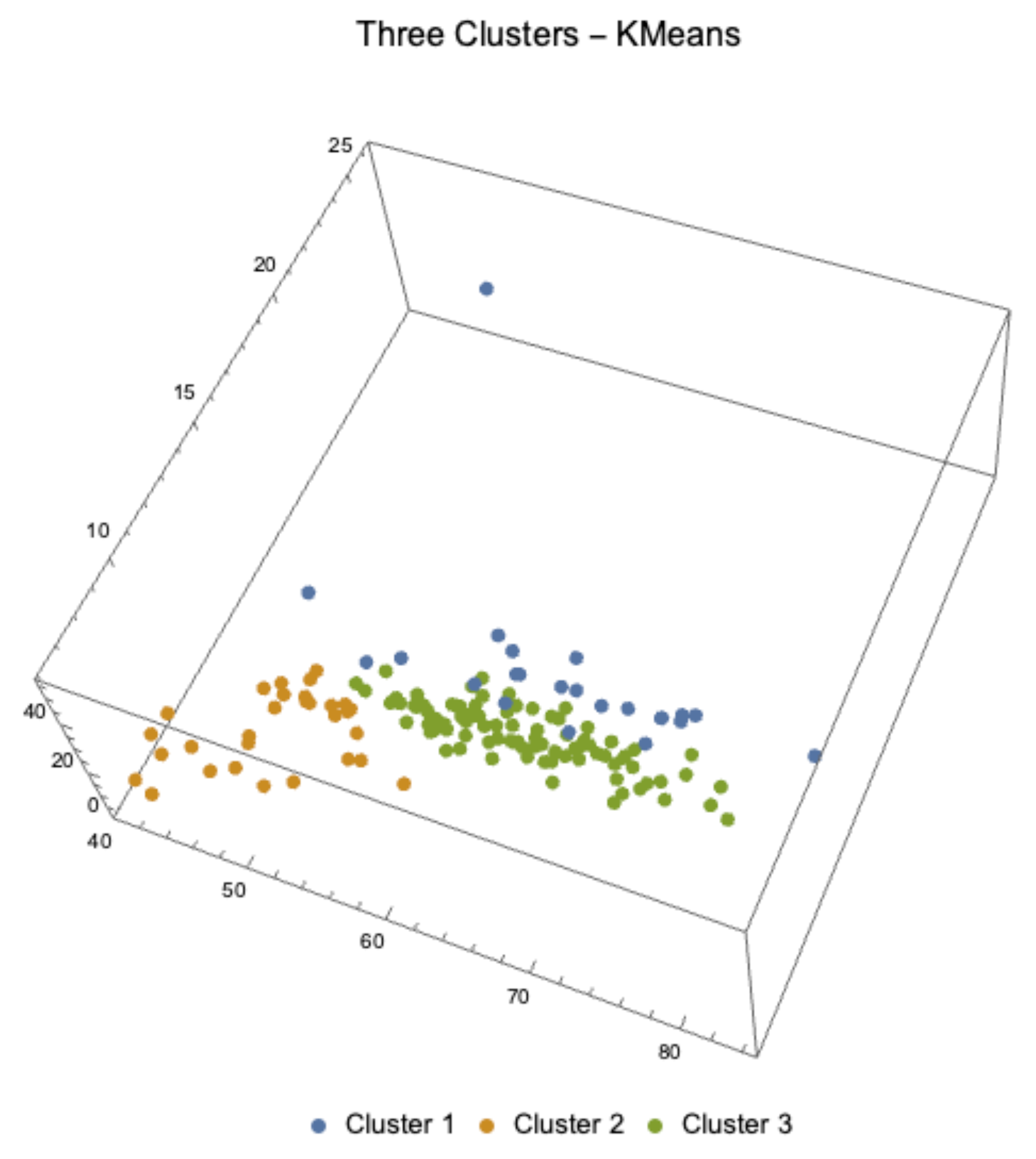
We first determine the data grouping in three clusters using the KMeans clustering classification method. A good introduction to classification techniques can be read in [21]. The results of the classification are presented in

Table 6. Subsets of varieties present in each cluster according to the 3 variables and 4 soils.

Types of Soil	Plant Height	Stem Diameter	Dry Matter
Soil 1: cluster varieties (a)	$\mathbf{1}:\mathcal{V}\setminus \{V_2,V_5,V_{16}\}$	$\mathbf{1}:\mathcal{V}\setminus \{V_2,V_5,V_{16}\}$	$\mathbf{1}:\mathcal{V}\setminus \{V_2,V_5,V_{16}\}$
	$\mathbf{2}:\varnothing$	$\mathbf{2}:\varnothing$	$\mathbf{2}:\varnothing$
	$\mathbf{3}:\{V_2,V_5,V_{16}\}$	$\mathbf{3}:\{V_2,V_5,V_{16}\}$	$\mathbf{3}:\{V_2,V_5,V_{16}\}$
Soil 2: cluster varieties	$\mathbf{1}:\left\{V_{14}\right\}$ (b)	$\mathbf{1}:\left\{V_{14}\right\}$ (b)	$\mathbf{1}:\left\{V_{14}\right\}$ (b)
	$\mathbf{2}:\mathcal{V}\setminus \{V_2,V_5,V_{16}\}$	$\mathbf{2}:\mathcal{V}\setminus \{V_2,V_5,V_{16}\}$	$\mathbf{2}:\mathcal{V}\setminus \{V_2,V_5,V_{16}\}$
	$\mathbf{3}:\{V_2,V_5,V_{16}\}$	$\mathbf{3}:\{V_2,V_5,V_{16}\}$	$\mathbf{3}:\{V_2,V_5,V_{16}\}$
Soil 3: cluster varieties	$\mathbf{1}:\varnothing$	$\mathbf{1}:\varnothing$	$\mathbf{1}:\varnothing$
	$\mathbf{2}:\mathcal{V}\setminus \{V_2,V_5,V_{16}\}$	$\mathbf{2}:\mathcal{V}\setminus \{V_2,V_5,V_{16}\}$	$\mathbf{2}:\mathcal{V}\setminus \{V_2,V_5,V_{16}\}$
	$\mathbf{3}:\{V_2,V_5,V_{16}\}$	$\mathbf{3}:\{V_2,V_5,V_{16}\}$	$\mathbf{3}:\{V_2,V_5,V_{16}\}$
Soil 4: cluster varieties	$\mathbf{1}:\mathcal{V}\setminus \{V_2,V_5,V_{16}\}$	$\mathbf{1}:\mathcal{V}\setminus \{V_2,V_5,V_{16}\}$	$\mathbf{1}:\mathcal{V}\setminus \{V_2,V_5,V_{16}\}$
	$\mathbf{2}:\varnothing$	$\mathbf{2}:\varnothing$	$\mathbf{2}:\varnothing$
	$\mathbf{3}:\{V_2,V_5,V_{16}\}$	$\mathbf{3}:\{V_2,V_5,V_{16}\}$	$\mathbf{3}:\{V_2,V_5,V_{16}\}$

^(a) The complete set of plant varieties is $\mathcal{V}=\{V_1,V_2,V_3,V_4,V_5,V_6,V_{11},V_{12},V_{13},V_{14},V_{15},V_{16}\}$. ^(b) One observation of variety $V_{14}$ appears in cluster $\mathbf{2}$; for Soil 2, we only consider two groups of varieties.

, and a graphical representation of the 3-dimensional clusters of observations is presented in Figure 4.

2.

As a consequence of the classification, we then use the grouping statistics $\mathcal{G}(12,2,9,3)$ and $\mathcal{G}(13,3,9,3,1)$ to assess for each one of the four soils the quality of the grouping. The values obtained are given in

Table 7. Values of the grouping statistic according to the 3 variables and 4 soils.

Types of Soil	Plant Height	Stem Diameter	Dry Matter
Soil 1	360	324	344
Soil 2	332	344	332
Soil 3	248 (a)	284 (a)	268 (a)
Soil 4	320	312	352

^(a) The 5% quantiles for the relevant distributions are: $q_{\mathcal{G}(12,2,9,3):0.05}=296=q_{\mathcal{G}(13,3,9,3,1):0.05}$.

.

3.

We then present some conclusions reached by the use of the statistics $\mathcal{G}(12,2,9,3)$ and $\mathcal{G}(13,3,9,3,1)$ to the results of the KMeans grouping.

Remark 8

(Analysis of the KMeans grouping in Table 6). It is relevant to notice that for all the three variables—plant height, stem diameter, and dry matter—the three clusters contain the same varieties. With the exception of Soil 2, the set of varieties $\mathcal{V}$ is always partitioned into two groups—each group in its own cluster—to wit, the set $\{V_2,V_5,V_{16}\}$ and the complement of this set with respect to $\mathcal{V}$, that is, $\mathcal{V}\setminus \{V_2,V_5,V_{16}\}$. The exception of Soil 2 is that the set of varieties $\mathcal{V}$ has variety $V_{14}$ in a cluster that is empty in the case of the other soils. Since the grouping statistic is applied to ranks of the varieties, obtained from the sums of all the observations in each variety, we discard the observation variety $V_{14}$ in cluster 1 for Soil 2. For Soil 2, the alternative of considering, instead of $\mathcal{G}(12,2,9,3)$, the grouping statistic $\mathcal{G}(13,3,9,3,1)$—corresponding to having one more rank—does not change the final result since the rank value corresponding to the $V_{14}$ variable is always equal to 13.

Remark 9

(Analysis of the statistic results in Table 7). Let us consider a statistical test using the statistical distribution $\mathcal{G}(12,2,9,3)$, where the null hypothesis is given as follows: the grouping produces inhomogeneous groups of varieties. We observe that the rejection region for this test consists of values of the statistic for sufficiently rank homogeneous groups. If the within-group ranks are homogeneous, the values of the statistic—given by Formula (1)—are smaller and so, given that the 5% quantile for the distribution $\mathcal{G}(12,2,9,3)$ is $q_{\mathcal{G}(12,2,9,3):0.05}=296$, we reject the null hypothesis—that the group is not homogeneous—for all the three variables, that is, plant height, stem diameter and dry matter, in Soil 3. This allow us to conclude that Soil 3 provides homogeneous production characteristics as given by the three variables’ values. In order to have a more detailed look at the particular behavior of Soil 3, we present in

Table 8. Subsets of ranks of varieties present in each cluster according to the 3 variables and 4 soils.

Types of Soil	Plant Height	Stem Diameter	Dry Matter
Soil 1: cluster ranks (a)	$\mathbf{1}:\mathcal{R}\setminus \{2,7,8\}$	$\mathbf{1}:\mathcal{V}\setminus \{8,9,11\}$	$\mathbf{1}:\mathcal{V}\setminus \{2,4,10\}$
	$\mathbf{2}:\varnothing$	$\mathbf{2}:\varnothing$	$\mathbf{2}:\varnothing$
	$\mathbf{3}:\{2,7,8\}$	$\mathbf{3}:\{8,9,11\}$	$\mathbf{3}:\{2,4,10\}$
Soil 2: cluster ranks (b)	$\mathbf{1}:\left\{13\right\}$ (c)	$\mathbf{1}:\left\{13\right\}$ (c)	$\mathbf{1}:\left\{13\right\}$ (c)
	$\mathbf{2}:{\mathcal{R}}^{\prime }\setminus \{1,5,11\}$	$\mathbf{2}:{\mathcal{R}}^{\prime }\setminus \{1,5,8\}$	$\mathbf{2}:{\mathcal{R}}^{\prime }\setminus \{3,10,11\}$
	$\mathbf{3}:\{1,5,11\}$	$\mathbf{3}:\{1,5,8\}$	$\mathbf{3}:\{3,10,11\}$
Soil 3: cluster ranks (a)	$\mathbf{1}:\varnothing$	$\mathbf{1}:\varnothing$	$\mathbf{1}:\varnothing$
	$\mathbf{2}:\mathcal{R}\setminus \{10,11,12\}$	$\mathbf{2}:\mathcal{R}\setminus \{1,11,12\}$	$\mathbf{2}:\mathcal{R}\setminus \{9,11,12\}$
	3 : {10, 11, 12}	3 : {1, 11, 12}	3 : {9, 11, 12}
Soil 4: cluster ranks (a)	$\mathbf{1}:\mathcal{R}\setminus \{1,8,12\}$	$\mathbf{1}:\mathcal{R}\setminus \{1,10,11\}$	$\mathbf{1}:\mathcal{R}\setminus \{3,5,11\}$
	$\mathbf{2}:\varnothing$	$\mathbf{2}:\varnothing$	$\mathbf{2}:\varnothing$
	$\mathbf{3}:\{1,8,12\}$	$\mathbf{3}:\{1,10,11\}$	$\mathbf{3}:\{3,5,11\}$

^(a) The complete set of possible ranks for plant varieties is $\mathcal{R}=\{1,2,3,4,5,6,7,8,9,10,11,12\}$. ^(b) The complete set of possible ranks for plant varieties is ${\mathcal{R}}^{\prime }=\{1,2,3,4,5,6,7,8,9,10,11,12,13\}$. ^(c) The rank for the observation of variety $V_{14}$ that appears in cluster $\mathbf{1}$; for Soil 2, we only consider two groups of varieties.

the ranks of the varieties in each cluster for all three variables.

Remark 10

(Analysis of the ranks of the varieties per clusters in Table 8). It is clear from the observation of the ranks (in red color) that the varieties in cluster 3 for Soil 3—$V_2,V_5,V_{16}$—perform homogeneously worse than the remaining varieties of the set $\mathcal{V}$ since the ranks are, in general, larger, the exception being variety $V_2$ for the variable stem diameter. Varieties $V_5,V_{16}$ have the second characteristic string CRG0314 in common—see Table A1 in the Appendix A—and so this may be an indication of the inadequacy of this ancestor characteristic of varieties $V_5,V_{16}$ to Soil 3.

5. Discussion

As stated in the first line of the introduction, a particular example of grouping distribution was used in [1], initially to allow the application of a well-known statistical methodology analysis and secondly to extract within-group homogeneity information of the grouping. In the present work, we studied the whole family of grouping distributions. Having observed severe computational challenges for the computation of the laws of grouping distributions—for large parameter values—we explored the possibility of an asymptotic result that would allow the determination of an approximate distribution for large parameter values. In order to obtain such an asymptotic result, we assumed some hypothesis heuristically deduced from the observation of the law behavior for small parameter values. It came as a surprise that under such a hypothesis, the asymptotic limit is a generalized function and not a measure that may be considered a probability distribution. Left with the problem of obtaining approximate distributions for the laws of grouping distributions, in the case of large parameter values, we proposed two methodologies that must be further studied since they present difficult technical implementation problems. In the context of Big Data, the grouping of variables and the determination of potential within-group homogeneities may represent a useful tool.

In this work, we deepened the study of some grouping distributions that find an important usage in testing the internal homogeneity—the within-group homogeneity—of subgroups of a given group. An example of such usage using real data was, presented and the comparison between the use of grouping statistics and the use of classic ANOVA highlighted the power of the grouping distributions to bring forward new information from the data. We pointed out the computational challenges arising from large values of the cardinal of the values to be grouped and the cardinal of the set of subgroups to consider—the main parameters of the grouping distribution—and aimed at a better understanding of the properties of the grouping distributions for large parameter values by several ways. In one of those ways, we proved that there does not exist an asymptotic result, giving a limit probability law when the main parameters tend to infinity and under a set of hypothesis that were observed in a significant set of examples. To contravene this negative result, we proposed, as implementation open problems, the ulterior study of two methodologies aimed at providing distribution approximations for large values of the main parameters.

6. Conclusions and Future Work

In this work, we formally defined and studied a family of discrete probability distributions—already introduced in a previous applied work—that may be used to assess the within-group homogeneity of a partition of observations in groups according to some criteria; examples of such criteria are the variables having some genetic common ascendent, and the values of the variables being grouped according to some clustering method such as KMeans. For the smaller values of the parameters, for which the computational effort is manageable, we provided tables of quantiles allowing to perform a test; the proposed test has as a null hypothesis that the group is not homogeneous. We also further developed a moment generating function result with a twofold purpose: firstly to analyze the possibility of an asymptotic result for the grouping distributions for large values of the parameters under some natural hypothesis, and secondly to assess the quality of a continuous approximation of the grouping distribution by a mixture of normal distributions. We presented an analysis of cocoa breeding experiment data, using an adequate grouping distribution, and we were able to extract information on the homogeneous behavior of cocoa plants production variables in one specific type of soil. By further analyzing the behavior of the variables grouping, we were able to conclude on the possible inadequacy of two variables in that specific type of soil.

There are at least three directions of development in the study of the grouping distributions. The first avenue is the development of the two methodologies proposed to provide distribution approximations for large values of the main parameters; this development may require an ingenious use of some optimization techniques. The second avenue is the investigation of the properties of the numerical semigroups associated to the sequence of convolutions of the grouping laws. And the third avenue is the quest for asymptotic results under different sets of hypotheses.

References

1. Opoku-Ameyaw, K.; Nunes, C.; Esquível, M.L.; Mexia, J.T. CMMSE: A nonparametric test for grouping factor levels: An application to cocoa breeding experiments in acidic soils. J. Math. Chem. 2023, 61, 652–672. [Google Scholar] [CrossRef]
2. Yitzhaki, S. Gini’s mean difference: A superior measure of variability for non-normal distributions. Metron 2003, 61, 285–316. [Google Scholar]
3. Zenga, M.; Polisicchio, M.; Greselin, F. The variance of Gini’s mean difference and its estimators. Statistica 2004, 64, 455–475. [Google Scholar]
4. Haye, R.L.; Zizler, P. The Gini mean difference and variance. Metron 2019, 77, 43–52. [Google Scholar] [CrossRef]
5. Baz, J.; Pellerey, F.; Díaz, I.; Montes, S. Stochastic ordering of variability measure estimators. Statistics 2024, 58, 26–43. [Google Scholar] [CrossRef]
6. Conover, W.J. Practical Nonparametric Statistics, 3rd ed.; John Wiley & Sons, Inc.: New York, NY, USA, 1999; pp. viii+584. [Google Scholar]
7. Butucea, C.; Tribouley, K. Nonparametric homogeneity tests. J. Stat. Plan. Inference 2006, 136, 597–639. [Google Scholar] [CrossRef]
8. Graham, R.L.; Knuth, D.E.; Patashnik, O. Concrete Mathematics: A Foundation for Computer Science, 2nd ed.; Addison-Wesley Publishing Company: Reading, MA, USA, 1994; pp. xiv+657. [Google Scholar]
9. Esquível, M.L. Probability generating functions for discrete real-valued random variables. Teor. Veroyatn. Primen. 2007, 52, 129–149. [Google Scholar] [CrossRef]
10. Rudin, W. Real and Complex Analysis, 3rd ed.; McGraw-Hill Book Co.: New York, NY, USA, 1987; pp. xiv+416. [Google Scholar]
11. Katznelson, Y. An Introduction to Harmonic Analysis; Dover Publications, Inc.: New York, NY, USA, 1976; corrected edition; pp. xiv+264. [Google Scholar]
12. Widder, D.V. The Laplace Transform; Princeton Mathematical Series; Princeton University Press: Princeton, NJ, USA, 1941; Volume 6, pp. x+406. [Google Scholar]
13. Schwartz, L. Mathematics for the Physical Sciences; Dover Publications, Inc.: Mineola, NY, USA, 1966; p. 358. [Google Scholar]
14. Kallenberg, O. Foundations of Modern Probability, 3rd ed.; Probability Theory and Stochastic Modelling; Springer: Cham, Switzerland, 2021; Volume 99, pp. xii+946. [Google Scholar] [CrossRef]
15. Schmüdgen, K. The Moment Problem; Graduate Texts in Mathematics; Springer: Cham, Switzerland, 2017; Volume 277, pp. xii+535. [Google Scholar]
16. Durrett, R. Probability—Theory and Examples, 5th ed.; Cambridge Series in Statistical and Probabilistic Mathematics; Cambridge University Press: Cambridge, UK, 2019; Volume 49, pp. xii+419. [Google Scholar] [CrossRef]
17. Beffa, F. Weakly Nonlinear Systems—With Applications in Communications Systems; Understanding Complex Systems; Springer: Cham, Switzerland, 2024; pp. xiv+371. [Google Scholar] [CrossRef]
18. Lindner, M. An introduction to the limit operator method. In Infinite Matrices and Their Finite Sections; Frontiers in Mathematics; Birkhäuser Verlag: Basel, Switzerland, 2006; pp. xv+191. [Google Scholar]
19. Ran, A.C.M.; Serény, A. The finite section method for infinite Vandermonde matrices. Indag. Math. 2012, 23, 884–899. [Google Scholar] [CrossRef]
20. Hernández-Pastora, J.L. On the solutions of infinite systems of linear equations. Gen. Relativ. Gravit. 2014, 46, 1622. [Google Scholar] [CrossRef]
21. Scitovski, R.; Sabo, K.; Martínez-Álvarez, F.; Ungar, Š. Cluster Analysis and Applications; Springer: Cham, Switzerland, 2021. [Google Scholar] [CrossRef]
Figure 1. Empirical distribution PDF of standardized X G ( 23 , 2 , 11 , 12 ) (blue) and fitting of the standardized data of the law of X G ( 23 , 2 , 11 , 12 ) by a normal distribution.
Mathematics 13 01805 g001
Figure 2. Linear fitting of the limit points of the logistic fittings for X G ( N , 2 , n 1 , n 2 ) considering N = 13 , 15 , 17 , 19 , 21 , 23 .
Mathematics 13 01805 g002
Figure 3. Logistic fitting of the first absolute values of moment ratios for X G ( 23 , 2 , 11 , 12 ) (left) and correspondent residuals (right).
Mathematics 13 01805 g003
Figure 4. Graphical representation of the 3 KMeans defined clusters in the three variables plant height, stem diameter and dry matter.
Mathematics 13 01805 g004