A Methodology to Extract Knowledge from Datasets Using ML

Abstract

This study aims to verify whether there is any relationship between the different classification outputs produced by distinct ML algorithms and the relevance of the data they classify, to address the problem of knowledge extraction (KE) from datasets. If such a relationship exists, the main objective of this research is to use it in order to improve performance in the important task of KE from datasets. A new dataset generation and a new ML classification measurement methodology were developed to determine whether the feature subsets (FSs) best classified by a specific ML algorithm corresponded to the most KE-relevant combinations of features. Medical expertise was extracted to determine the knowledge relevance using two LLMs, namely, chat GPT-4o and Google Gemini 2.5. Some specific ML algorithms fit much better than others for a working dataset extracted from a given probability distribution. They best classify FSs that contain combinations of features that are particularly knowledge-relevant. This implies that, by using a specific ML algorithm, we can indeed extract useful scientific knowledge. The best-fitting ML algorithm is not known a priori. However, we can bootstrap its identity using a small amount of medical expertise, and we have a powerful tool for extracting (medical) knowledge from datasets using ML.

1. Introduction

Each ML algorithm produces a different output for the same input. The input may be a whole dataset or a subset of the features (FS) of the dataset. The classifying power may be interpreted as the ‘goodness’ of the FS.

However, there is some confusion about the meaning of ‘goodness’ in this context. Usually, it means FSs that are useful to build a good predictor (of the class of the dataset, i.e., with a high classification score). On the other hand, it can mean finding all potentially relevant features [1]. This relevance vs. usefulness distinction is not always well-discriminated and depends on what we mean by relevance [2,3].

No ML algorithm is clearly better than the others. However, their different classification results may have some meaning. If we encode (medical) knowledge for a given dataset, we may determine whether different classifying algorithms behave better than others, with respect to knowledge relevance, in order to extract such encoded knowledge.

The aim of this paper is to encode medical knowledge relevance to test whether there are significant differences among ML algorithms to learn that knowledge and, if so, to use the most efficient ML algorithm on a given dataset for extracting useful and relevant medical knowledge.

Importantly, ML algorithms can learn correlations, and correlation does not imply causation. However, the goal of ML models is often a guide to action. Moreover, correlation is a sign of a potential causal connection, and we can use it as a guide for further investigation [4]. For this reason, medical professionals in everyday clinical practice must validate the potential causality suggested by ML algorithms as knowledge extracted from datasets.

The aim of this paper is different from that of the related task of Feature Selection (FS). In FS, the goal is to obtain feature subsets that produce the best classification performance [5]. At most, they search for feature subsets that have the same class distribution as the whole dataset and a very good classification performance [6,7].

The aim of this paper is also related to that of ML interpretability. However, our intention is not to interpret the results of ML as opposed to black boxes [8], but to serve as a guide to extract knowledge from datasets, and to our best knowledge this is the first work on which the results of ML classification are directly compared to a measure of the codification of knowledge in feature subsets extracted from datasets.

A secondary objective of this research is to assess the quality of datasets using ML, i.e., to test whether the different ML algorithms cannot extract knowledge because they are not statistically validated.

2. Materials and Methods

In this section, we introduce a methodology to validate an original dataset using a probability distribution of datasets extracted from it and then apply the methodology to the validated original datasets.

We introduce in Section 2.1 a method called dataset feature splitting (DFS) to generate a probability distribution of working datasets out of an original dataset under study (see

Table 1. Principal characteristics of the four original datasets used in this study.

	Feature Types	Missing Data	Class Distribution	Instances
HP-UCI	1 CAT/9 NUM	NO	75/540	615
HF-UCI	5 CAT/7 NUM	NO	96/203	299
HD-UCI	4 CAT/8 NUM	NO	138/161	299
CKD-UCI	4 CAT/9 NUM	NO	43/115	158

and Appendix A for a description of the original datasets used in this research). In Section 2.2, we introduce a method to compute the classification performance using ordered lists of all possible combinations of FSs and seven different supervised ML algorithms belonging to important scientific families of algorithms (see Appendix B for a description of these algorithms). In Section 2.3, we introduce a method to encode scientific medical knowledge of a dataset using pairs (tuples) of medical features’ knowledge that is relevant to the class of the dataset, using two important LLMs. In Section 2.4, we compare the encoded medical knowledge to the ordered lists of classification performance in order to evaluate how well the different ML algorithms classify the relevant knowledge. In Section 2.5, we describe the validation of the probability distribution generation and the ML knowledge performance results. In Section 2.6, we apply the entire methodology to the original datasets that passed its distribution validation.

Figure 1 depicts the general pipeline of the methodology through the four main components: DFS, FS ranking, LLM-based knowledge encoding, and ML relevance evaluation.

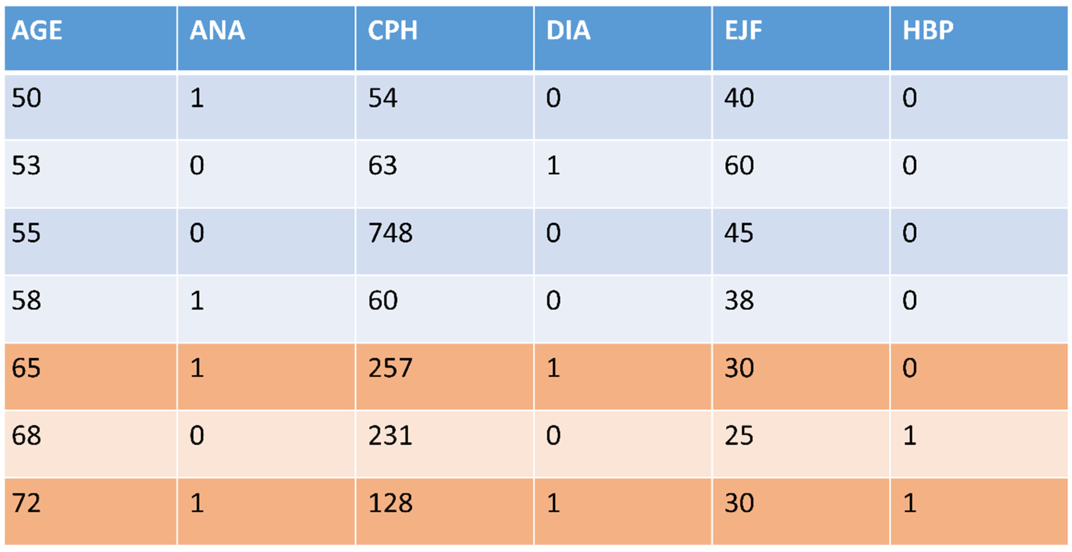
2.1. Dataset Generation over a Probability Distribution: Dataset Feature Splitting (DFS)

Because we intend to measure the knowledge relevance of FSs and then assess the relationship to the classification score of the same FSs, we need different datasets with the same features (columns) extracted from the same probability distribution, i.e., holding a stationary assumption [9].

For this purpose, we developed dataset feature splitting (DFS). It operates as follows: Let us assume that we are studying lactose intolerance in Eastern populations [10]. We would be interested in one dataset of people from the East (e.g., Japan) and another from people not considered Eastern. For instance, if we had a dataset of people from across the world, and one of the features (columns) was the geographic origin (say Japan/not Japan), we would divide the dataset according to that column to obtain two different datasets, one from Japan and the other from the remainder of the world, extracted from the same probability distribution.

Figure 2 illustrates the process using a fragment of data from one of the datasets [11] used in this study. The first column (AGE) provides the sorting of the dataset; we generated two different datasets (different colors) by dividing column AGE using the threshold of 65 years old (people under 65 years old and people over this age). Box 1 shows the methodology systematically.

Box 1. Dataset feature splitting.

Select a column (feature) from the set of features of the dataset

    Sort the dataset using that column

    Set a threshold in the ordered column

    Divide the dataset into two parts (higher and lower datasets)

Table 1 summarizes the properties of the four original datasets used in this research, i.e., their feature types, missing data, class distribution, and total number of instances.

Some columns, such as DIA or ANA, are 1/0 columns in which patients have or do not have this feature (diabetes or anemia). Other columns are numeric (e.g., diastolic blood pressure, DBP), and their values are real numbers. In this case, the column was classified according to high or low feature values. Meaningful clinical limits were used to compute the classification thresholds.

In general, if we have a medical dataset of 12 medical features (except the class), we may construct a maximum of 24 different datasets dividing two-fold across each feature (column), extracted from the same population probability distribution.

It is important to notice the presence of many kinds of bias in medical datasets. These biases range from sampling bias (the dataset does not represent the entire population) to measurement bias (when there are systematic errors based on the method to measure the variables), including selection bias (when some groups are more or less likely to be included, for many reasons) or historical bias based on historical inequalities or practices that are encoded in data. Probably for this reason, out of the four distributions generated using DFS in this study, only three of them have been validated and have passed the Kolmogorov-Smirnov statistical test to detect if the generated datasets belong or not to the same probability distribution, see below.

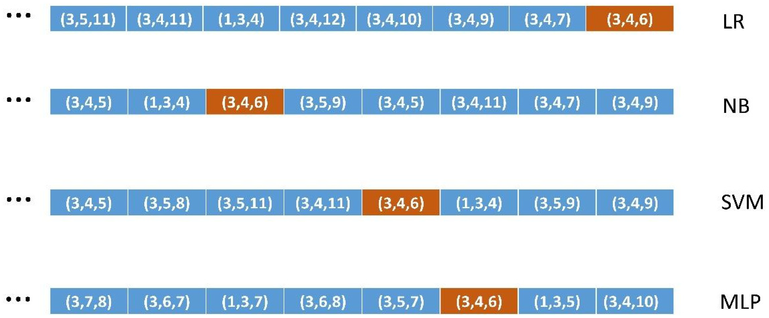
2.2. An Objective Measure of Classification Performance: Ordered Lists of All Combinations of FS of a Given Size

In order to measure the FS classification performance on each ML algorithm, we propose the following method.

Each ML algorithm produces a different classification result for the same FS. We need an exact measure of how well a given-sized FS classifies for a given ML algorithm. Thus, we need to compute all combinations of FSs of a given size. In addition, in order to compare their classification power, we build F-measure-ordered lists for each important size (3, 4, 5, and 6) and each ML algorithm.

For instance, in Figure 3, we depict the ordered lists of four of the seven algorithms [12,13] used in this study for the case of FSs of size 3. We can see that FS (3, 4, 6) has different positions in the different algorithms. Thus, to test how well a given ML algorithm classifies an FS of a given size, we determined its position in the corresponding ordered list (same FS size and same ML algorithm). Box 2 shows the ordered lists building the methodology systematically.

Box 2. Ordered list building.

For each ML algorithm

    For each FS size 3 through 6

      Compute the weighted F measure of the supervised ML execution

      Add it to the sorted list corresponding to each combination (ML algorithm, FS size)

Because DFS may have produced datasets with heavily skewed class distributions, we mitigated that effect using resampling techniques such as SMOTE (synthetic minority over-sampling technique) [14] in order to rebalance the datasets. We used oversampling when the ratio of the minority versus majority class was under 0.2. Specifically, we used SMOTE with all the DFS datasets generated out of the original HP-UCI dataset (see its class distribution in Table 1) and some DFS datasets extracted from the original HD-UCI dataset.

We have preferred to use oversampling of the minority class such as in SMOTE rather than other possible techniques such as under-sampling the majority class or adjusting category weights since our datasets are not very large and we have obtained very good results with SMOTE from the beginning.

This approach is computationally expensive and may not scale for working datasets of more than 12 to 15 features (columns). This study performed a proof of concept with a maximum of 12 features. This means that, for instance, there were C (12, 3) = 220 FSs of size 3, 495 of size 4, 792 of size 5, and 924 of size 6. This means that the length of the ordered lists grows unbound, as combinatorial numbers when the number of columns of the dataset is greater than 12–15. Since each combination performed a calculation of seven ML algorithms (some 2–3 s), and all combinations were executed for each working dataset generated through DFS, this took about (220 + 495 + 792 + 924) × 3 × 10 = 72,930 s, i.e., 20.26 h for the HP-UCI distribution on standard workstation hardware, since the HP-UCI distribution has generated ten different datasets.

In order to address datasets of more than 20–30 columns, we would have to use parallel computing with tens or hundreds of CPUs working simultaneously in order to obtain a reasonable execution time. This means using hardware available only in supercomputing centers to extract knowledge from large datasets in a systematic way. On the other hand, since the tasks are very similar (essentially equal), the program to control the parallel execution turns out to be straightforward.

2.3. Encoding Knowledge Relevance: Using Medical Expertise from LLMs

In order to determine how well the different MLs classify the knowledge-relevant FSs, we need an assessment of the FS relevance extracted from some source of medical expertise.

In this study, we queried two different LLMs [15,16] (Chat GPT -4o [17] and Google Gemini 2.5 [18]) in order to encode the knowledge relevance of pairs of features (FSs of size 2), that is, whether there was a relationship between the pairs of features (columns of a dataset) with respect to the medical outcome of the dataset.

For instance, in the Heart Failure (HF) dataset, where we have one feature, diabetes (column DIA, categorical), and another feature, anemia (column ANA, categorical), the posed query might be as follows:

“Is there a synergic relationship between diabetes and anemia to suffer heart failure?”

If such a relationship exists, we would tag ‘1, relevant’ as the pair (2, 4) corresponding to the features of anemia and diabetes (see Appendix A). Otherwise, it would be tagged ‘0, non-relevant’.

Box 3 shows the medical knowledge encoding methodology systematically.

Box 3. Medical knowledge encoding.

For each working dataset generated using DFS, with one driving feature Fi

    For each remaining feature in the dataset Fj

      Query an LLM to check whether the pair (Fi, Fj) is medical knowledge-relevant or not

      If yes, add Fj to the list of relevant features with respect to Fi

Table 2. Working datasets of the four probability distributions with the list of relevant features with respect to the DFS driving feature of each dataset, according to the responses of the two LLMs used.

HP-UCI		HF-UCI
AGE H	(4, 5, 6, 7, 10, 11)	AGE H	(2, 3, 4, 6, 7, 9, 10, 11)
SEX H	(5)	ANA H	(1, 3, 4, 5, 6, 7, 8, 9, 10, 11)
SEX L	(3, 10)	CPH H	(1, 2, 4, 6, 9, 11)
ALB L	(4, 5, 6, 7, 11, 12)	DIA H	(1, 2, 3, 5, 6, 7, 8, 9, 10, 11)
ALP H	(1, 3, 5, 6, 7, 9, 10, 11, 12)	EJF L	(1, 2, 3, 4, 6, 7, 8, 10, 11)
ALT H	(1, 2, 3, 4, 6, 7, 9, 10, 11, 12)	HBP H	(1, 2, 3, 4, 7, 9, 10, 11)
BIL H	(1, 3, 4, 5, 6, 11, 12)	PLA H	(1, 2, 4, 6, 10, 11)
CHO L	(4, 5, 6, 11)	SCR H	(1, 2, 3, 4, 5, 6, 7, 11)
CRE H	(1, 4, 5, 6, 12)	SSO H	(1, 2, 3, 4, 6, 10, 11)
PRO H	(3, 4, 5, 6, 7, 10, 11)	SEX H	(6, 7)
		SEX L	(1, 2, 4, 9, 11)
HD-UCI		SMO H	(1, 2, 3, 4, 6, 7, 9, 10)
AGE H	(2, 3, 4, 5, 7, 8, 9, 10, 11, 12)
SEX H	(5, 8, 10, 11, 12)	CKD-UCI
SEX L	(1, 4, 6, 7, 9)	AGE H	(2, 3, 4, 6, 7, 8)
BPS H	(1, 2, 5, 6, 7, 8, 9, 10, 11, 12)	URE H	(1, 3, 4, 5, 6, 7)
FBS H	(1, 2, 4, 7, 9, 10, 11, 12)	CRE H	(1, 2, 4, 5, 6, 8)
ECG H	(2, 4, 7, 8, 9, 10)	SOD L	(1, 2, 3, 5, 6, 8)
MHR H	(1, 2, 4, 5, 6, 8, 9, 10, 11, 12)	POT H	(2, 3, 4, 6, 8)
ANG H	(1, 2, 4, 6, 7, 9, 10, 12)	HEM L	(1, 2, 3, 4, 5, 7, 8)
STD H	(1, 2, 4, 5, 6, 7, 8, 10, 11, 12)	WHI H	(1, 2, 6, 8)
SLO H	(1, 2, 4, 5, 6, 7, 8, 9, 11, 12)	RED L	(1, 3, 4, 5, 6, 7)
CA H	(1, 2, 4, 5, 7, 9, 10, 12)
CHO H	(1, 2, 4, 5, 7, 8, 9, 10, 11)

shows the CRE H dataset of the HP-UCI probability distribution, which represents the patients in the original HP-UCI dataset that have high levels of creatinine. The original dataset was divided according to the CRE column (numeric) into those patients with a high level of creatinine (CRE H) and those with a low level (CRE L). Table 2 shows the list of features (columns) that are knowledge-relevant with respect to each DFS-driving feature (CRE, for instance).

The medical relevance assessments between feature pairs extracted from Chat GPT -4o and Gemini 2.5 may be relative. Note that we are mainly interested in the relative differences between distinct ML algorithms. This means that, when coding the pairs of relevant/non-relevant features, we also interpreted the responses of the LLMs to the queries relatively. This means that if the LLM returned an emphatically affirmative response, we took the feature pair as relevant, but if the LLM was unsure about the relationship, we interpreted it as non-relevant since we needed to establish a difference.

We also needed to take into account that, in our original datasets on Hepatitis C, for instance, all features tended to be relevant individually with respect to the medical outcome, so it was difficult to obtain non-relevant feature pairs, but we needed them in order to establish a relative difference between the ML algorithms.

In addition, we used two different LLMs in order to obtain a vote: we produced one result only if the two LLMs agreed. If one of the two was incorrect, it would be unlikely for both to be, at least on the same subject.

Supplementary Material S1 contains several examples of queries posed to Chat GPT-4o and Gemini 2.5 and the responses used in this research, using the interpretation described above.

The lists of knowledge-relevant (pairs of) features in Table 2 have been revised by a medical professional (see Acknowledgements). Even though it is difficult for clinicians to hardly discriminate between medical features in relation to the medical outcome of each dataset; and also the opinion of specialists in hepatitis and heart problems is needed; she has confirmed the validity of the lists in Table 2 in about 85–90% of the cases. This proportion is in agreement with the 10 to 25% non-concordance among medical practitioners when diagnosing diseases based on features suffered by patients [19].

2.4. How Well Do the Different ML Algorithms Classify the Most Relevant Binary FSs?

Next, we were able to compute how well the different ML algorithms classified the medical knowledge-relevant FS pairs, by determining their ordinal position in the ordered lists.

From Table 2, we have, for each dataset of the probability distribution, the list of features that were knowledge-relevant to the driving DFS feature of the dataset. For instance, in the HP (hepatitis C) probability distribution, the dataset CRE H (high level of creatinine) had feature 4, alkaline phosphatases (ALP), as relevant, among others.

In order to test how well features 10 (CRE) and 4 (ALP), which were mutually relevant for the Hepatitis C probability distribution, were classified, we counted how high the number ‘4’ rated in the four ordered lists of the dataset CRE H (the CRE is feature 10). Conversely, we counted how high the number ‘10’ rating was in the four ordered lists of the dataset ALP H (ALP is feature 4).

Rather than calculating this individually, we counted, for each dataset representing one specific feature, how highly rated the total number of its relevant features (the numbers in the lists of Table 2) was. These numbers were summed, accumulated, and averaged for each of the four ordered lists (FS sizes 3, 4, 5, and 6), since the ordered list length depends on the size of its FSs, and the maximum produced a best-classifying ML algorithm per ordered list. Box 4 shows this method in a systematic form.

Box 4. ML algorithms’ relevance.

For each of the seven ML algorithms

    For each working dataset and its driving medical feature Fi

      For each feature Fj in its list of medical knowledge relevant features

          For each of the four sizes of F-measure-sorted lists

                Obtain and accumulate the position of Fj in the F-measure-sorted list

    Return the ML algorithm with the maximum accumulated for each size

Table 3. Classification and knowledge relevance scores of the seven ML algorithms for the case of the CRE H dataset corresponding to the Hepatitis C probability distribution.

CRE H
size 3	156.3 (SVM)	151.3 (RF)	149.8 (DT)	147.6 (NB)	146.6 (KN)	133.0 (LR)	132.7 (MLP)
size 4	470.2 (SVM)	446.8 (RF)	445.0 (DT)	443.2 (NB)	441.9 (KN)	424.4(MLP)	408.9 (LR)
size 5	926.6 (SVM)	892.5 (KN)	879.2 (RF)	878.4 (NB)	874.6 (DT)	841.0(MLP)	825.3 (LR)
size 6	1273.0 (SVM)	1245.4(KN)	1218.3 (NB)	1210.7 (RF)	1206.0 (DT)	1181.0(MLP)	1157.0 (LR)

shows the specific case of the CRE H dataset. For each ordered list (FS sizes 3 through 6), there was a best ML algorithm (leftmost) and a descending ordering of algorithms to the right.

It is important to notice that some ML algorithms behave better than others for different specific datasets. This would mean that the statistical nature of datasets makes one algorithm or another perform best on them. This is the reason why we have used seven very different ML algorithms that cover the whole spectrum of distinct scientific families of ML algorithms. We have used one representative of classical statistics methods (Logistic Regression); methods based on information theory (Decision Tree); algorithms based on Bayesian statistics (Naïve Bayes); methods based on linear models or neural networks (Multilayer Perceptron); algorithms based on linear models with non-linear transformations (Support Vector Machine); methods based on instance-based learning (K-Nearest Neighbor); and finally ensemble algorithms based on computations on many basic algorithms (Random Forest, based on many Decision Trees).

This is the way to find the set of ML algorithms that best classify the FSs that have the combinations of features most relevant to scientific medical knowledge for each dataset probability distribution under study.

2.5. Validation Methodology

2.5.1. Validation of Method 1 (DFS)

Each original dataset had a distribution P(X), and the working datasets extracted from them using DFS had conditional distributions P(X|X_j ≤ t) or P(X|X_j ≥ t), where t was the threshold used to divide the original dataset if feature X_j had a meaning under that threshold or over it, respectively.

In order to determine whether the working datasets represented the same distribution, we used the Kolmogorov–Smirnov (KS) test [20]. This is the standard statistical method to test whether groups of datasets belong to the same probability distribution. The input to the KS test was one working dataset (ALP H, for instance) and the original HP-UCI dataset. Then, it produced a p-value per working dataset.

Table 4. Detail of Table 5, showing the p-values returned by the KS test on two datasets of the HP-UCI distribution.

DFS Datasets	p-Values
ALP H	1.1394834474 × 10−5
CRE H	4.2769255669 × 10−26

(detail of

Table 5. The p-values returned by the KS test applying the Benjamini–Hochberg correction. Datasets returning p-values approximately greater than threshold 8.33 × 10⁻⁶ are considered to belong to the same probability distribution.

HP-UCI	4 out of 10	HF-UCI	10 out of 12
AGE H	1.0892849424 × 10−5	AGE H	0.00058360217226
SEX H	5.1118124321 × 10−6	ANA H	0.00352660750438
SEX L	1.9878513331 × 10−19	CPH H	0.59033279794372
ALB L	9.6008360198 × 10−26	DIA H	0.00765360026050
ALP H	1.1394834474 × 10−5	EJF L	4.7648532405 × 10−7
ALT H	4.3517379024 × 10−46	HBP H	0.00058360217226
BIL H	1.4937625445 × 10−5	PLA H	0.00018288992313
CHO L	1.8795587161 × 10−19	SCR H	0.59033279794372
CRE H	4.2769255669 × 10−26	SSO H	4.7648532405 × 10−7
PRO H	2.2151976407 × 10−22	SEX H	0.00018288992313
		SEX L	0.00178955624413
HD-UCI	9 out of 12	SMO H	0.12566168302727
AGE H	0.66297421392268
SEX H	0.01899680622953	CKD-UCI	0 out of 8
SEX L	1.4733907068 × 10−8	AGE H	4.6913601105 × 10−31
BPS H	0.00468751862537	URE H	1.6302989587 × 10−33
FBS H	0.01116685752824	CRE H	2.0841286358 × 10−30
ECG H	0.00204213738762	SOD L	1.6087231294 × 10−42
MHR H	8.6014095603 × 10−11	POT H	2.0841286358 × 10−30
ANG H	0.01899680622953	HEM L	3.0897650452 × 10−47
STD H	1.1199214677 × 10−6	WHI H	2.1831400120 × 10−21
SLO H	0.22253198035961	RED L	3.4672730092 × 10−40
CA H	6.8454149810 × 10−9
CHO H	0.07620693805287

) shows the p-values returned by the KS test applied to the ALP H and CRE H working datasets of the HP-UCI distribution. The Benjamini–Hochberg correction [21] was applied in order to control the expected number of false positives. It is commonly applied when the KS test is applied to a number of datasets. It sorts the p-values and applies a dynamic threshold.

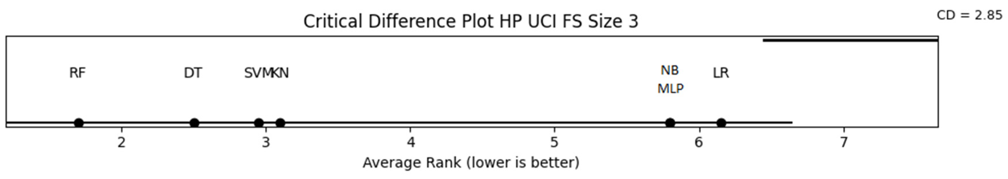
2.5.2. Validation of Methods 2, 3, and 4

Table 6. Seven vectors of results of the averaged position in the ordered lists of each ML algorithm in the HP-UCI distribution with FS size 3.

HP-3	AGE H	SEX H	SEX L	ALB L	ALP L	ALT H	BIL H	CHO H	CRE H	PROTH
LR	172.6	24.36	50.31	185.37	256.16	280.24	199.22	133.61	132.97	209.00
NB	173.12	29.19	44.66	182.4	254.48	282.13	210.93	133.49	147.63	201.87
SVM	191.0	31.05	50.31	192.34	264.6	291.9	216.22	137.22	156.27	218.21
MLP	182.65	25.48	43.1	185.91	258.53	280.4	199.61	133.59	132.66	212.15
DT	193.09	29.07	51.15	193.26	268.13	293.11	217.32	135.70	149.81	220.55
KN	192.90	29.92	52.43	191.4	265.88	289.31	211.28	137.35	146.64	219.80
RF	193.36	29.42	52.47	192.82	270.33	294.63	219.22	133.73	151.34	221.07

shows seven vectors of results, one per ML algorithm, corresponding to the averaged ordinal positions of significant features in the ordered list of each working dataset of the HP-UCI distribution and one specific FS size case, namely, size 3.

Since we were working with numerical values (i.e., non-categorical), we could not validate the statistical significance of these results using the chi-square test [22]. We had to use a robust non-parametric method such as the Friedman test [23], which in addition did not require the normality of data. This test produced a p-value of 6.981233636665472 × 10⁻⁸ for the case of the HP UCI distribution with FS size 3 (Table 6).

Table 7. The p-values returned by the Friedman test on the four distributions.

	Size 3	Size 4	Size 5	Size 6
HP	6.981233 × 10−8	9.286800 × 10−8	1.877473 × 10−6	0.0001678653
HF	9.261686 × 10−7	2.554832 × 10−8	2.544815 × 10−7	3.296192 × 10−7
HD	0.0769675283	0.0325569482	0.0325569482	0.1000616722
CKD	0.3713981664	0.4664793246	0.2683203192	0.1442754291

shows the p-values of the four distributions under statistical significance validation. We further applied the post hoc Nemenyi test [24] to obtain a ranking of algorithms to determine which was the best algorithm for each probability distribution. Figure 4 shows the Critical Difference (CD) plot from the Nemenyi test comparing the algorithms in the HP-UCI distribution for FS size 3. RF was the best algorithm. In addition, the CD established a threshold to compare algorithms [24]. Those differing less than the CD threshold (2.85 in Figure 4) with respect to the best were also considered significant. Supplementary Material S2 contains the 12 CD plots corresponding to the three valid distributions.

Table 8. The valid algorithms for the three distributions were obtained using the CD threshold of each CD plot.

HP-UCI	HF-UCI	HD-UCI
RF, DT, SVM, KN	DT, NB, LR, RF	RF, KN, SVM, NB, DT

summarizes the ML algorithms that fall within the CD margin from the best algorithm for each distribution.

2.6. Application of the Methodology: Knowledge Extraction from the Original Datasets

The Kolgomorov–Smirnov and Friedman tests can be used to filter out non-valid distributions. It is remarkable that both tests coincided with three valid and one non-valid distribution. Out of the four distributions produced and analyzed in this research, three of them (HP, HF, and HD) passed the KS and the Friedman tests, while the CKD distribution failed in the two tests, confirming it was not suitable for the methodology.

With the three valid distributions, we applied the methodology to the three original datasets that produced them, using DFS. Note that Box 1 (DFS) was applied to generate the testing distributions, so we obviated it. We applied Box 2 to the three successful original datasets (HP-UCI, HF-UCI, and HD-UCI) in order to build their four ordered lists (one per FS size from 3 through 6). We used the pairs of features produced previously by Box 3, applied to the whole probability distributions of the original datasets, in order to apply Box 4 to each of the three original datasets. Then, we determined the ordinal positions of the two features of each pair in the four ordered lists. Note that we checked for pairs of features rather than for individual features as in Section 2.4. This means that we tested whether each relevant pair (two features) was a subset of each FS in the ordered lists (three, four, five, and six features).

Box 4 produced an ordering of the ML algorithms per ordered list (FS size) and for each dataset as shown in

Table 9. The order of the ML algorithms for each original valid dataset and FS size.

HP
size 3	170.5 (KN)	170.0 (RF)	169.5 (DT)	167.7 (SVM)	157.6 (LR)	155.7 (NB)	155.3 (MLP)
size 4	759.0 (KN)	757.3 (DT)	755.9 (SVM)	755.1 (RF)	719.6 (MLP)	713.6 (LR)	700.0 (NB)
size 5	2011.6 (SVM)	2003.8 (KN)	1997.4 (DT)	1995.8 (RF)	1943.9 (MLP)	1912.5 (LR)	1864.4 (NB)
size 6	3511.9 (SVM)	3477.1 (RF)	3477.1 (KN)	3474.2 (DT)	3402.4 (MLP)	3365.4 (LR)	3268.4 (NB)
HF
size 3	268.9 (DT)	264.2 (RF)	244.5 (KN)	227.0 (NB)	218.8 (SVM)	211.9 (MLP)	203.5 (LR)
size 4	1208.5 (DT)	1190.6 (RF)	1072.8 (KN)	1022.9 (NB)	1008.2 (SVM)	968.1 (MLP)	937.9 (LR)
size 5	3179.7 (DT)	3115.8 (RF)	2776.2 (KN)	2744.1 (SVM)	2706.2 (NB)	2600.5 (MLP)	2553.0 (LR)
size 6	5481.8 (DT)	5391.9 (RF)	4872.2 (SVM)	4826.8 (KN)	4712.2 (NB)	4587.9 (MLP)	4547.1 (LR)
HD
size 3	229.3 (KN)	226.1 (RF)	225.3 (MLP)	224.3 (LR)	223.9 (DT)	223.6 (NB)	223.2 (SVM)
size 4	1051.3 (KN)	1048.2 (RF)	1043.9 (MLP)	1042.0 (SVM)	1041.5 (LR)	1035.2 (NB)	1031.5 (DT)
size 5	2849.9 (MLP)	2847.7 (RF)	2840.4 (LR)	2839.7 (KN)	2837.7 (SVM)	2830.7 (NB)	2792.5 (DT)
size 6	5069.7 (MLP)	5054.8 (RF)	5051.1 (NB)	5043.6 (KN)	5041.6 (SVM)	5036.4 (LR)	4958.1 (DT)

for the three successful datasets.

Table 10. Best classified FS (front of the ordered list) for each best ML algorithm of Table 9 (only the relevant ML algorithms). Note that we have respected the positions of the algorithms in the ordering of Table 9.

HP-UCI
FS size 3	(5, 6, 7) KN	(4, 5, 6) RF	(4, 5, 6) DT	(5, 6, 9) SVM
FS size 4	(4, 5, 6, 12) KN	(4, 5, 6, 10) DT	(5, 6, 9, 12) SVM	(4, 5, 6, 10) RF
FS size 5	(4, 6, 9, 11, 12) SVM	(4, 5, 6, 10, 12) KN	(4, 5, 6, 7, 11) DT	(5, 6, 7, 10, 11) RF
FS size 6	(3, 4, 5, 6, 11, 12) SVM	(4, 5, 6, 7, 10, 11) RF	(4, 5, 6, 9, 11, 12) KN	(3, 4, 5, 6, 10, 11) DT
HF-UCI
FS size 3	(5, 8, 11) DT	(2, 3, 8) RF		(1, 5, 12) NB
FS size 4	(4, 5, 8, 11) DT	(3, 8, 9, 10) RF		(2, 3, 5, 12) NB
FS size 5	(3, 4, 8, 9, 10) DT	(3, 4, 8, 9, 10) RF
FS size 6	(1, 3, 6, 8, 9, 11) DT	(3, 5, 6, 7, 8, 10) RF
HD-UCI
FS size 3	(3, 10, 11) KN	(3, 10, 11) RF
FS size 4	(3, 4, 10, 11) KN	(3, 8, 10, 11) RF		(3, 8, 10, 11) SVM
FS size 5	(2, 3, 9, 11, 12) MLP	(2, 5, 8, 10, 11) RF		(3, 4, 5, 10, 11) KN
FS size 6	(1, 3, 8, 9, 10, 11) MLP	(1, 2, 3, 8, 10, 11) RF	(2, 3, 7, 8, 9, 11) NB	(3, 4, 8, 9, 10, 11) KN

shows the best-classified FS (front of the ordered list) for each best ML algorithm of Table 9, restricted to the relevant algorithms that fell within the threshold of the CD of the whole distribution (see Table 8 for the ML algorithms of the three distributions).

Table 11. Best FS extracted for each dataset using the relevant ML algorithms of Table 10 (left-hand columns) and significant features extracted from those FSs (right-hand columns).

HP-UCI		HF		HD
4, 5, 6	ALP, ALT, AST	5, 8, 11	EJF, SCR	3, 10, 11	CP, SLO, CA
4, 5, 6, 10	CRE	3, 8, 9, 10	CPH, SSO, SEX	3, 8, 10, 11	ANG
4, 5, 6, 10, 12	PRO	3, 4, 8, 9, 10	DIA	3, 4, 5, 10, 11	BPS, FBS
4, 5, 6, 10, 11, 12	GGT	3, 4, 5, 8, 9, 10

summarizes (in the left-hand columns) the best FS extracted for each dataset using the relevant ML algorithms in Table 10. Several algorithms may be applied to extract those FSs from Table 10; however, determining those algorithms is beyond the scope of this research, and we leave it for future work. In our design, we established an upper limit of six features in the right-hand columns.

This means that, for instance, for the HP-UCI distribution features, ALP (alkaline phosphatase), ALT (alanine amino-transferase), and AST (aspartate amino-transferase) were most significant in combination for Hepatitis C, followed by CRE (creatinine), PRO (protein), and GGT (gamma-glutamyl transpeptidase). We could achieve something similar with the HF-UCI and the HD-UCI datasets.

As stated before, there are correlations between features, but they suggest potential causalities. These results are suggestions to be validated via clinical practice by medical professionals in order to be considered scientific medical knowledge.

3. Results

3.1. Results of Methods

In the first part of the methodology (generation of a probability distribution to determine the validity of each original dataset), we generated a number of working datasets using Box 1 (DFS).

Each working dataset represented a DFS driving feature. In addition, each working dataset had four F-measure ordered lists (one per FS size) generated through Box 2. Box 3 generated a list of knowledge-relevant features with respect to the DFS driving feature after the responses of the LLMs (Chat GPT and Google Gemini).

Table 2 summarizes the lists of features resulting from Box 3 for each working dataset for each probability distribution.

Those datasets formed selecting the high values of the driving feature have the suffix H (high), while the datasets formed selecting the low values are suffixed L (low). Note that some datasets have both suffixes, namely, SEX, in order to have datasets corresponding to both males and females of the distribution.

Some dataset-driving features were not used because the DFS-resulting datasets were not well-formed, i.e., all the instances (patients) of the datasets belonged to the same unique class, making it impossible to perform ML classification experiments. This is why, for instance, the HP-UCI distribution has 12 features, but there are only 10 working datasets.

The list of features in Table 2 represents the numbers that were searched for their positions in the four ordered lists of each ML algorithm using Box 4.

Table 12. The order of the ML algorithms produced by each probability distribution and FS size according to the results obtained from the CD plots of the Nemenyi test.

HP-UCI		HF-UCI
Size 3	RF, DT, SVM, KN, NB, MLP, LR	Size 3	DT, NB, LR, RF, MLP, KN, SVM
Size 4	RF, DT, SVM, KN, MLP, NB, LR	Size 4	NB, DT, LR, RF, KN, MLP, SVM
Size 5	RF, SVM, DT, KN, MLP, NB, LR	Size 5	NB, DT, LR, RF, MLP, KN, SVM
Size 6	RF, SVM, KN, DT, MLP, LR, NB	Size 6	NB, DT, LR, RF, MLP, KN, SVM
HD-UCI		CKD-UCI
Size 3	RF, KN, SVM, NB, DT, MLP, LR	Size 3	N/A
Size 4	RF, DT, KN, NB, SVM, MLP, LR	Size 4	N/A
Size 5	RF, DT, NB, SVM, KN, MLP, LR	Size 5	N/A
Size 6	RF, SVM, NB, DT, KN, MLP, LR	Size 6	N/A

shows the ordering of ML algorithms produced by each probability distribution and FS size according to the results obtained from the CD plots of the Nemenyi test. The CD plots can be found in CD Plots produced by the post-hoc Nemenyi test on the three valid probability distributions, and Table 8 summarizes the valid algorithms for the three distributions, obtained using the Critical Difference (CD) threshold of each CD plot.

3.2. Validation of Methods

3.2.1. Validation of Method 1 (DFS)

Following the validation methodology outlined in Section 2.5.1, Table 5 summarizes the p-values returned by the KS test applied to each working dataset extracted using DFS with respect to the original UCI dataset corresponding to each probability distribution. Taking into account that we are dealing with a hard disruption of the original dataset, we set up an initial threshold of 0.0001 (10⁻⁴) to separate datasets belonging to the same distribution. Because we executed a high number of tests, we applied a Bonferroni correction [25] of 10 or 12, depending on the distribution, and we had a threshold of approximately 8.33 ×10⁻⁶. This threshold clearly divided the distributions into two groups, datasets belonging or not belonging to the distribution, as stated in the upper rows of Table 5.

3.2.2. Validation of Methods 2, 3, and 4

As in the validation methodology outlined in Section 2.5.2, Table 7 summarizes the results of the p-values of the non-parametric Friedman test for the four probability distributions and the four FS sizes. Clearly, the HP, HF, and HD UCI distributions produced significant results, while the CKD UCI distributions did not, i.e., they yielded p-values well over the 0.05 significance limit.

We know from Table 7 that the HP, HF, and HD UCI original datasets were valid, and we could apply the methodology in order to extract useful medical knowledge.

Table 5 and Table 7 show that DFS (Box 1) may be used to validate a dataset since those valid datasets using it were also validated by Box 2, Box 3, and Box 4 using the non-parametric robust Friedman test. This fact saves time and works in the methodology since we can discard invalid datasets using the Kolmogorov–Smirnov test on the datasets produced by DFS. However, we needed to apply Box 2, Box 3, and Box 4 on the valid probability distributions (i.e., not only in the original datasets), because we needed to identify the subset of valid ML algorithms using the CD plot produced by the post hoc Nemenyi test after the Friedman test. Then, we applied Box 2, Box 3, and Box 4 to the original datasets.

4. Discussion

The proposed methodology to extract (medical) knowledge from datasets using ML comprises four main methods. The validation of Box 1 (DFS) on the probability distribution it generates, using the Kolmogorov–Smirnov test, remarkably produced the same results as the validation of Box 2, Box 3, and Box 4 using the Friedman test on the same probability distribution.

In fact, the validation of Box 1 using the Kolmogorov–Smirnov test and the validation of Box 2, Box 3, and Box 4 using the Friedman test in this research served as double validation of the methodology, since they produced the same results, i.e., they produced the same valid datasets.

As a result, we used the validation of DFS using the KS test as the main validation of datasets, but we still needed to apply Box 2, Box 3, and Box 4 to the whole probability distributions (not only to the valid original datasets). This is because the application of the Friedman test to the whole distribution is still necessary to apply the post hoc Nemenyi test and obtain the subset of valid ML algorithms produced by the CD threshold in the CD plots generated by the test.

The fact that each probability distribution had a different set of valid ML algorithms suggests that these different sets of ML algorithms depend on the statistical nature of each dataset and that of its associated probability distribution generated by DFS. This is the reason why the seven ML algorithms cover the wide spectrum of the different types of available scientific families of algorithms.

Once we determined the results of Box 4 (ML relevance evaluation), it was straightforward to extract useful feature correlations to be validated by medical professionals as medical knowledge. However, as stated above, several algorithms may be applied to those relevant FS results; the conception of these algorithms is beyond the scope of this research, and we leave it as future work.

It is also important to keep in mind that we are dealing with statistical data, for instance in the ordered lists of FSs, and we do not need to exclusively consider the very first FS of each list but could extend the algorithms to consider the k few best classified and use k as a parameter of these algorithms.

It is also important to note the imitative nature of the LLMs used to encode medical knowledge out of pairs of medical features [26,27,28]. LLMs are not able to reason about medical knowledge and causality but just respond according to the documents on which they were trained. This is why the correct interpretation of the responses of the two LLMs (see Section 2.3) used is so important. In addition, using two different LLMs serves to prevent hallucination by only taking as good their responses when both interpretations coincide in the same result.

Limitations and Further Work

One limitation of this study is the use of two-wise relationships (pairs of features) to encode medical knowledge. However, checking for three-wise or higher-order relationships would be cumbersome, both because of their high number and because of their inherent complexity. We assume that two-feature relationships (FSs) should be good enough to trigger the differences in the relevance vs. classification score of the seven ML algorithms, taking into account that we seek to determine the relative differences between ML algorithms.

However, the main limitation of this study might be the time- and effort-consuming task of validating medical knowledge against real medical practice. This process may take years to reach a consensus in the international scientific medical community.

Therefore, interesting future work would be to process well-known medical data distributions to analyze, validate, extract, systematize, and start contrasting medical knowledge with the experience of years of practice in scientific medicine.

This could be accomplished in an almost encyclopedic fashion, intending to classify, extract, and systematize scientific (medical) knowledge. It may take a long time, but it may be worthwhile.

5. Conclusions

We have created and demonstrated a new methodology whereby different-classifying ML algorithms may fit or adapt to different-natured medical datasets using best-classifying FSs that are most knowledge-relevant with respect to the class or outcome of the dataset.

This methodology can determine whether a given dataset is valid to extract knowledge from using one subset of standard supervised ML algorithms. If so, the best-fitting ML algorithms subset can be used to extract and systemize medical knowledge from the dataset.

The subset of best-fitting ML algorithms suggests a number of correlations that are potential causalities, and medical professionals must validate these as scientific knowledge through medical practice.

This can be a powerful tool to extract and systematize (medical) scientific knowledge out of the fast-growing number of (medical) datasets available.

The medical scientific community must validate the results through clinical practice. It may take a long time, but it may be worthwhile.

References

1. Guyon, I.; Elisseeff, A. An introduction to variable and feature selection. J. Mach. Learn. Res. 2003, 3, 1157–1182. [Google Scholar]
2. Blum, A.L.; Langley, P. Selection of relevant features and examples in machine learning. Artif. Intell. 1997, 97, 245–271. [Google Scholar] [CrossRef]
3. Kohavi, R.; John, G.H. Wrappers for feature selection. Artif. Intell. 1997, 97, 273–324. [Google Scholar] [CrossRef]
4. Domingos, P. A few useful things to know about machine learning. Commun. ACM 2012, 55, 78–87. [Google Scholar] [CrossRef]
5. Liu, H.; Yu, L. Toward integrating feature selection algorithms for classification and clustering. IEEE Trans. Knowl. Data Eng. 2005, 17, 491–502. [Google Scholar]
6. Dash, M.; Liu, H. Feature Selection for Classification. Intell. Data Anal. 1997, 1, 131–156. [Google Scholar] [CrossRef]
7. Kononenko, I. Estimating Attributes: Analysis and Extensions of RELIEF. In Proceedings of the European Conference on Machine Learning (ECML-94), Catania, Italy, 6–8 April 1994; Springer: Berlin/Heidelberg, Germany, 1994. [Google Scholar]
8. Molnar, C. Interpretable Machine Learning, 2nd ed.; Lulu Enterprises, Inc.: Durham, NC, USA, 2022; Available online: https://christophm.github.io/interpretable-ml-book/ (accessed on 20 May 2025).
9. Bishop, C.M. Pattern Recognition and Machine Learning; Springer: New York, NY, USA, 2006. [Google Scholar]
10. Swallow, D.M. Genetic influences on lactase persistence and lactose intolerance. Annu. Rev. Genet. 2003, 37, 197–219. [Google Scholar] [CrossRef] [PubMed]
11. UC Irvine Machine Learning Repository. Available online: https://archive.ics.uci.edu/ (accessed on 26 March 2025).
12. Witten, I.H.; Frank, E.; Hall, M.A.; Pal, C.J. Data Mining: Practical Machine Learning Tools and Techniques; Morgan Kaufmann: Burlington, Massachusetts, MA, USA, 2016. [Google Scholar]
13. Pedregosa, F.; Varoquaux, G.; Gramfort, A.; Michel, V.; Thirion, B.; Grisel, O.; Blondel, M.; Prettenhofer, P.; Weiss, R.; Dubourg, V.; et al. Scikit-learn: Machine learning in Python. J. Mach. Learn. Res. 2011, 12, 2825–2830. [Google Scholar]
14. Chawla, N.V.; Bowyer, K.W.; Hall, L.O.; Kegelmeyer, W.P. SMOTE: Synthetic minority over-sampling technique. J. Artif. Intell. Res. 2002, 16, 321–357. [Google Scholar] [CrossRef]
15. Zhou, S.; Xu, Y.; Zhang, M.; Xu, C.; Guo, Y.; Zhan, Y.; Ding, S.; Wang, J.; Xu, K.; Fang, Y.; et al. Large Language Models for Disease Diagnosis: A Scoping Review. arXiv 2024, arXiv:2409.00097. [Google Scholar]
16. Nazi, Z.A.; Peng, W. Large Language Models in Healthcare and Medical Domain: A review. arXiv 2024, arXiv:2401.06775. [Google Scholar] [CrossRef]
17. OpenAI. ChatGPT (v2.0) [Large Language Model]. OpenAI. 2025. Available online: https://openai.com/chatgpt (accessed on 26 March 2025).
18. Google AI. Gemini: A Tool for Scientific Writing Assistance. 2025. Available online: https://gemini.google.com/ (accessed on 26 March 2025).
19. Elmore, J.G.; Longton, G.M.; Carney, P.A.; Geller, B.M.; Onega, T.; Tosteson, A.N.; Nelson, H.D.; Pepe, M.S.; Allison, K.H.; Schnitt, S.J.; et al. Diagnostic concordance among pathologists interpreting breast biopsy specimens. JAMA 2015, 313, 1122–1132. [Google Scholar] [CrossRef] [PubMed]
20. Massey, F.J., Jr. The Kolmogorov-Smirnov test for goodness of fit. J. Am. Stat. Assoc. 1951, 46, 68–78. [Google Scholar] [CrossRef]
21. Benjamini, Y.; Hochberg, Y. Controlling the false discovery rate: A practical and powerful approach to multiple testing. J. R. Stat. Soc. Ser. B (Methodol.) 1995, 57, 289–300. [Google Scholar] [CrossRef]
22. Pearson, K. On the criterion that a given system of deviations from the probable in the case of a correlated system of variables is such that it can be reasonably supposed to have arisen from random sampling. Philos. Mag. 1900, 50, 157–175. [Google Scholar] [CrossRef]
23. Friedman, M. A comparison of alternative tests of significance for the problem of m rankings. Ann. Math. Stat. 1940, 11, 86–92. [Google Scholar] [CrossRef]
24. Demšar, J. Statistical comparisons of classifiers over multiple datasets. J. Mach. Learn. Res. 2006, 7, 1–30. [Google Scholar]
25. Dunn, O.J. Multiple comparisons among means. J. Am. Stat. Assoc. 1961, 56, 52–64. [Google Scholar] [CrossRef]
26. Bender, E.M.; Gebru, T.; McMillan-Major, A.; Shmitchell, S. On the Dangers of Stochastic Parrots: Can Language Models Be Too Big? In Proceedings of the 2021 ACM Conference on Fairness, Accountability, and Transparency, FAccT’21, Toronto, ON, Canada, 3–10 March 2021. [Google Scholar]
27. Nori, H.; King, N.; McKinney, S.M.; Carignan, D.; Horvitz, E. Capabilities of GPT-4 on Medical Challenge Problems. arXiv 2023, arXiv:2303.13375. [Google Scholar]
28. Liebrenz, M.; Schleifer, R.; Buadze, A.; Bhugra, D. Generative AI in Healthcare: Point of View of Clinicians; McKinsey & Company: New York, NY, USA, 2023. [Google Scholar]
Figure 1. The four main components of the KE methodology.
Mathematics 13 01807 g001
Figure 2. A fragment of the HP-UCI dataset used in this study. It was split into two datasets (different colors) through its feature AGE using the threshold of 65 years old.
Mathematics 13 01807 g002
Figure 3. The ordered lists of features of size 3 with the relative position of the feature (3, 4, 6) on each list for four of the seven ML algorithms used.
Mathematics 13 01807 g003
Figure 4. Critical Difference plot after the Nemenyi test for the HP UCI distribution with FS size 3. The CD value in this case is 2.85. The best ML algorithm has been RF (on the left) and those ML algorithms differing less than the Critical Difference CD (2.85), i.e., DT, SVM, and KN, are considered the set of the best-fitting ML algorithms for this distribution (HP-UCI) and FS size (3).
Mathematics 13 01807 g004