TANS: A Tolerance-Aware Neighborhood Search Method for Workflow Scheduling with Uncertainties in Cloud Manufacturing

Abstract

In this paper, we consider the workflow scheduling problem with soft deadlines and fuzzy time uncertainties in cloud manufacturing environments. Workflow tasks in cloud manufacturing often involve uncertain execution and logistics times due to large-scale and geographically distributed resources, creating significant challenges for efficient and reliable scheduling. To address these challenges, we propose the Tolerance-aware Neighborhood Search (TANS) algorithm, which integrates fuzzy time quantization with heuristic neighborhood search techniques. A comprehensive workflow scheduling architecture is established, and multiple neighborhood structures and heuristic search methods are developed to systematically explore feasible solutions. The effectiveness of TANS is verified by extensive experiments and parameter calibrations based on Analysis of Variance (ANOVA). Experimental results indicate that TANS reduces workflow delays by 39% on average compared to state-of-the-art methods, demonstrating high efficiency in scenarios with different numbers of tasks and resources.

1. Introduction

Cloud manufacturing (CMfg) has emerged as an advanced service-oriented manufacturing paradigm, allowing geographically distributed resources to collaboratively provide efficient and scalable manufacturing services [1]. With the proliferation of Industry 4.0 technologies, more and more manufacturing enterprises rely on CMfg platforms to fulfill diverse production demands. Typically, workflow scheduling in CMfg involves allocating a large number of heterogeneous manufacturing tasks to geographically dispersed manufacturing resources [2,3], significantly impacting production efficiency, resource utilization, and customer satisfaction. Optimizing workflow scheduling in CMfg environments is critical not only to improve resource allocation efficiency but also to enhance the competitive advantage of manufacturing enterprises. However, real-world manufacturing environments are inherently uncertain, involving fuzzy execution and logistics times, which considerably complicate scheduling activities. For example, in a distributed automotive part manufacturing scenario, tasks such as CNC machining (uncertain execution time: 2 to 4 h) and cross-facility logistics (fuzzy delay: 1 to 3 h) must be coordinated with a 24 h soft deadline. Traditional methods do not handle such uncertainties, leading to 15–30% deadline violations [1].

In this paper, we specifically address the problem of workflow scheduling with soft deadlines under fuzzy time uncertainties within the CMfg environment. Unlike traditional deterministic workflow scheduling problems that assume exact execution and logistics times [4,5,6], the problem studied explicitly considers fuzzy uncertainty, represented by triangular fuzzy numbers. The scope of our research includes tasks constrained by predefined soft deadlines and resources characterized by heterogeneous execution capabilities and geographically distributed logistics constraints. The primary optimization objective is to minimize the total fuzzy delay in the workflow, measured by the difference between the fuzzy workflow completion time and the given soft deadline. Although previous work has explored deterministic or stochastic scheduling extensively, workflow scheduling considering fuzzy uncertainties with soft deadlines, especially in CMfg scenarios, remains largely unexplored. Therefore, our research represents a novel “leaf node” in the fuzzy workflow scheduling research tree in CMfg.

Scheduling workflows under fuzzy timing and soft deadlines in CMfg is inherently challenging due to several critical factors. First, the fuzziness of task execution times and logistics durations results in uncertainty propagation across workflow tasks, making precise task scheduling extremely difficult. Second, workflows usually exhibit complex task dependencies, leading to partial-order constraints that significantly restrict feasible task arrangements and scheduling flexibility. Balancing the allocation of tasks to optimize logistics costs against task execution efficiency creates a profound contradiction: assigning tasks to geographically closer services reduces logistics time but may result in suboptimal resource utilization, whereas prioritizing faster execution services often significantly increases logistics overhead. Finally, soft deadlines introduce another layer of complexity by allowing acceptable but not strictly enforced task delays, complicating the trade-off between efficiency and practicality. Therefore, effective handling of these intertwined challenges requires sophisticated modeling and novel optimization approaches.

To effectively tackle the above-mentioned challenges, this paper proposes a TANS algorithm, designed explicitly to address workflow scheduling under fuzzy timing and soft deadlines in CMfg environments. Specifically, the main contributions of this paper are summarized as follows:

(i)  

To handle the fuzzy uncertainty in task execution and logistics times, we propose a fuzzy quantization model based on triangular fuzzy numbers. This model effectively quantifies and controls the propagation of fuzziness through workflow tasks, mitigating the impact of uncertainty on scheduling performance.

(ii) 

To deal with complex partial-order task constraints and soft deadlines, we develop fuzzy sub-deadline partitioning strategies and a maximum sub-workflow time consumption priority strategy. These strategies systematically prioritize tasks, ensuring feasible task scheduling sequences that effectively minimize total delays.

(iii)

Addressing the trade-off between execution efficiency and logistics overhead, we propose a comprehensive tolerance-aware neighborhood search optimization framework, including novel neighborhood structure construction operators and adaptive search strategies. This approach efficiently explores the solution space, balancing task allocation and logistics optimization.

The remainder of this paper is organized as follows. The related work is described in Section 2. Section 3 details the model and the formulation of the problem. The proposed fuzzy scheduling optimization methods based on TANS are elaborated on in Section 4. The experimental results and comprehensive analyses are given in Section 5, followed by conclusions and suggestions for future research directions in Section 6.

2. Related Work

The issue of scheduling in cloud manufacturing has been extensively investigated by scholars. This segment will present a summary of current studies concerning the topics addressed in this paper, with an emphasis on three main areas: workflow scheduling in cloud manufacturing, workflow scheduling under uncertainty, and workflow scheduling with soft deadline constraints.

2.1. Workflow Scheduling in Cloud Manufacturing

Workflow scheduling in cloud manufacturing is a typical NP-hard problem, for which the academic community has already achieved many excellent research outcomes. In the realm of heuristic scheduling, Zhu et al. [2] considered both the deadline and cost of products in cloud manufacturing, proposing a cloud manufacturing scheduling optimization algorithm based on non-cooperative games. Ma et al. [3] established a manufacturing service scheduling model for industrial cloud robots (ICRs) and introduced a Digital Twin (DT) enhanced scheduling optimization mechanism and a manufacturing service scheduling method based on an improved discrete differential evolution (IDDE) algorithm. Li et al. [4] addressed the cloud manufacturing scheduling problem under logistics resource constraints, proposing an improved Grey Wolf Optimization (IGWO) algorithm to minimize the maximum completion time (makespan) considering queuing in logistics transportation. Bi et al. [5] designed a multi-agent dynamic optimization scheduling system framework in response to the dynamic distribution of cloud resources and the real-time requirements of cloud tasks in the cloud manufacturing environment.

In the area of metaheuristic scheduling, Zhang et al. [6] took into account the interests of manufacturing resource demand enterprises and cloud platform operators, constructing a multiobjective optimization resource allocation model representing the interests of both parties in the cloud environment, and solved model instances based on a dynamic neighborhood algorithm. Liu et al. [7] proposed a game theory based on task scheduling and model selection for effective exploitation of distributed manufacturing resources in CMfg, where the Nash Equilibrium (NE) is achieved through a Dual Ant Colony Optimization (DACO) algorithm. This approach allows the services offered by different providers to handle a batch of tasks in real time. In addition, to meet the needs of different service providers and applicants, this method considers multiple task attributes, including completion time, cost, service quality, service composition capability, service availability, energy consumption, service sustainability, service maintainability, and service trustworthiness.

In the domain of reinforcement learning-based scheduling, Zhang et al. [8] modeled the distributed real-time scheduling problem of various services as a semi-Markov decision process, considering both the processing of service ordering and the distribution of logistics services, and proposed a distributed real-time scheduling method for cloud manufacturing based on deep reinforcement learning. Yang et al. [9] introduced a novel and efficient edge-cloud Digital Twin (DT) manufacturing system inspired by resource scheduling techniques. They modeled the adaptive optimization problem as a dynamic programming problem and proposed a new Cooperative Clustering Parallel Q-Learning (CCPQL) algorithm, which reduced the total delay with a higher convergence rate.

2.2. Workflow Scheduling Under Uncertainty

In the field of workflow scheduling with uncertainty in a cloud computing environment, there exists considerable research. Lin et al. [10] proposed a cost-driven scheduling strategy in fuzzy edge-cloud environments, representing resource performance and bandwidth using triangular fuzzy numbers. By preprocessing and merging partial critical paths, this strategy effectively reduces data transmission costs and task execution expenses, showing improved real-time performance and robustness in uncertain conditions. Yang et al. [11] addressed workflow scheduling problems with unknown task execution times and convex Time Utility Functions (TUFs). They integrated machine learning-based predictions with greedy optimization, using multilayer perceptron networks to estimate task execution times and linear programming to relax nonpreemption constraints. Their greedy algorithm significantly improves total utility and offers the first polynomial-time approximation solution for convex TUFs. Rajput et al. [12] focused on scheduling Spark workflow tasks in multicloud networks. Their heuristic-based method considered the heterogeneity of VM instances, priority constraints, and performance uncertainties, significantly reducing execution costs while effectively meeting workflow deadlines. The experimental results indicated a performance improvement of more than 50% compared to existing approaches.

Compared to precise scheduling, research on fuzzy scheduling in cloud manufacturing is relatively limited, focusing primarily on the traditional manufacturing domain, with particular emphasis on studies concerning time-related fuzzy factors. Wang et al. [13] addressed uncertainties caused by uncontrollable factors in the energy-saving hybrid flow shop scheduling problem (HFSP) and proposed a Non-dominated Sorting Genetic Algorithm -II (NSGA-II) with dual optimization objectives to minimize both fuzzy manufacturing span and total fuzzy energy consumption. Sun et al. [14] integrated batch splitting into the flexible assembly job shop scheduling problem, utilizing L-R fuzzy numbers with nonlinear membership functions to describe the time uncertainties of scheduling problems, and introduced a batch splitting-based L-R fuzzy flexible assembly job shop scheduling problem (BFFAJSP). Zhou et al. [15] viewed the parallel casting workshop scheduling problem as an unrelated parallel machine scheduling (UPMS) problem inherently featuring fuzzy order processing times, and for a multi-objective integer programming model, they proposed a new Pareto-based discrete particle swarm optimization (PDPSO). Zhang et al. [16] considered the trade-off between transportation efficiency and unknown transportation time discovery rate in multiobjective evolutionary algorithms (MOEAs) referring to emergency resource scheduling scenarios. Congcong et al. [17] focused on the precision and timeliness of the delivery of workshop material in uncertain environments, dynamically adjusting material delivery time windows based on intelligent logistics technology, and proposed a dynamic optimization method for the distribution of intelligent material using a hybrid heuristic algorithm.

2.3. Workflow Scheduling with Soft Deadline Constraints

In the field of cloud computing task scheduling, there exists considerable research on soft and hard deadline constraints. Tasks with hard deadlines strictly require processing within their delay limits, whereas tasks with soft deadlines can afford some flexibility with their deadlines. The performance of cloud computing systems depends not only on the accuracy of the results but also on the timeliness of their availability. In the cloud computing environment, Fizza et al. [18] proposed a scheduling strategy to choose the most appropriate task offloading locations (including local embedded systems, fog/edge, or cloud) for tasks with hard or soft deadline constraints. Mukherjee et al. [19] explored a pricing model for the offloading of soft and hard tasks according to the deadline in mobile edge computing and derived the optimal pricing scheme using backward induction. He et al. [20] considered both delay-sensitive applications (i.e., tasks with hard deadlines) and computation-intensive applications (such as tasks with soft deadlines) and designed an offloading strategy to maximize the number of tasks that meet their deadlines. Xin et al. [21] studied the task-offloading problem with mixed (hard/soft) deadlines in edge computing, proposing two algorithms with competitive ratios during the task-offloading and task execution order adjustment stages, respectively. Yao et al. [22] developed a memetic algorithm-based scheduling strategy (KDMA). They combined heuristic local search operators with multiobjective metaheuristics to optimize workflow execution cost and makespan. Extensive evaluations of real-world workflow instances demonstrated substantial overall performance advantages and excellent generalization capabilities. Cai et al. [23] proposed an urgency-based list scheduling algorithm (ULS) to dynamically schedule interleaved workflows in heterogeneous computing systems. ULS prioritizes tasks based on real-time execution information, effectively reducing deadline miss rates and overall tardiness compared to existing methods, thus addressing resource contention and quality-of-service degradation in dynamic environments.

Cloud manufacturing, as a derivative of cloud computing, also features discussions and studies on soft and hard deadline constraints in the domain of cloud manufacturing task scheduling. Yorie N et al. [24] aimed to solve the problem of dynamically adjusting service capacity to match workload laws by using soft demands and soft deadline constraints to describe service capacity’s steady mean and minimum variance distribution strategy, deriving the Pareto optimal conditions for a distributed strategy balancing service capacity variance and mean square.

Comparative analysis of related works on workflow scheduling are listed in

Table 1. Comparative analysis of related works on workflow scheduling.

Method	Application Environment	Uncertainty Model	Deadline Type	Advantages	Disadvantages
Zhu et al. (2022) [2]	Cloud Manufacturing	Deterministic	Hard	Clear cost optimization	Ignores time/logistics uncertainty
Ma et al. (2020) [3]	Industrial Cloud Robots	Deterministic	Hard	Digital Twin integration; real-time feedback	Limited scalability; no fuzzy handling
Li et al. (2021) [4]	Cloud Manufacturing and Logistics	Deterministic/ Stochastic	Hard	Effective logistics optimization	Moderate scalability; lacks fuzzy uncertainty
Lin et al. (2025) [10]	Edge-Cloud Environments	Fuzzy (TFNs)	Soft	Robust fuzzy logistics handling	Moderate scalability; limited resource optimization
Yang et al. (2024) [11]	Cloud Workflow Scheduling	Stochastic (ML predictions)	Soft	Effective prediction-based scheduling	Computationally intensive; requires training data
Rajput et al. (2024) [12]	Multicloud Networks	Stochastic	Mixed	Significant cost-performance improvement	Ignores fuzzy uncertainties
Wang et al. (2023) [13]	Hybrid Flow Shop Scheduling	Fuzzy	Hard	Minimizes fuzzy energy consumption	High computational complexity
Sun et al. (2023) [14]	Flexible Assembly Scheduling	Fuzzy (L-R fuzzy numbers)	Hard	Effective fuzzy assembly handling	Limited flexibility; computationally demanding
Zhou et al. (2022) [15]	Parallel Casting Workshop	Fuzzy (UPMS model)	Hard	Effective fuzzy optimization	Not cloud-oriented; computationally complex
Yao et al. (2024) [22]	Workflow Scheduling	Deterministic/ Stochastic	Soft	Effective heuristic–metaheuristic combination	Limited fuzzy uncertainty handling
Proposed TANS	Cloud Manufacturing	Fuzzy (TFNs)	Soft	Robust uncertainty handling; adaptive heuristic; good scalability	/

. In summary, while previous work has made notable progress in modeling task uncertainties and optimizing workflow scheduling under hard deadlines, soft deadline scenarios with realistic logistics and execution uncertainty remain underexplored. For example, prior works like Zhu et al. [2] optimized costs via game theory but ignored logistics uncertainty, while Ma et al. [3] used digital twins without addressing soft deadlines. Unlike prior deterministic methods, TANS introduces tolerance-aware fuzzy sub-deadline partitioning (Section 4.2) and composite neighborhood structures (Section 4.5.3), allowing dynamic trade-offs between execution efficiency and logistics overhead. The proposed TANS framework addresses these gaps by offering a comprehensive and flexible solution tailored for cloud manufacturing, thus contributing new insights to the field.

3. System Model

3.1. System Architecture

The systematic framework for workflow scheduling in cloud manufacturing is illustrated in Figure 1. It involves three major entities: Users, Cloud Manufacturing Service Platform, and Manufacturers. Users submit workflow applications via the platform’s interface, where each workflow consists of a series of heterogeneous sub-tasks with partial-order constraints and varying workloads. Upon submission, the Task Manager analyzes the user’s request, performs fuzzy time parameter estimation for each task, divides the overall deadline into fuzzy sub-deadlines, and generates a task scheduling sequence. Inputs of the Task Manager are Workflow DAG and soft deadline D. The output of the task manager is fuzzy sub-deadlines ${\tilde{d}}_i$. Simultaneously, the Resource Manager oversees a geographically distributed and heterogeneous service resource pool, calculates fuzzy execution times and interresource logistics costs, maintains up-to-date information on resource availability and workload, and provides these data in real time to the scheduler. The scheduler comprises two components: the Allocator, which assigns resources to tasks based on the predefined sequence and a matching strategy, and the Adjuster, which refines the schedule using a tolerance-aware neighborhood search algorithm to minimize total workflow delay. The input of the Allocator is task sequence. The output of the Allocator is resource assignments $x_{ij}$. Finally, the Executive implements the optimized schedule and provides execution feedback to both users and service providers.

The architecture adheres to ISO 22400 [25] for manufacturing system metrics and IEEE 1855-2016 [26] for fuzzy logic modeling.

For the problem considered in this study, we make the following assumptions.

• At the workflow level, users submit workflow applications with soft deadline constraints to the cloud manufacturing platform. Both the soft deadlines and the topological structure of the workflows are predefined and known in advance, and they do not change during the scheduling process. All workflows are final upon submission and cannot be modified or resubmitted.
• At the task level, the total number of tasks contained within a workflow application, as well as the workload of each task, is predefined and known in advance, and it remains unchanged during the scheduling process.
• At the service resource level, the execution speed of each service and the logistic time between different services are fuzzy and uncertain values. The quantity of services, execution speeds, and logistics times between different services are predefined and known in advance and do not change during the scheduling process. There is no logistic time for the same service.
• During the scheduling process, only the execution time and logistics time of the tasks are considered, while the setup time of the tasks is ignored. A task can only be executed by one service resource, and it cannot be interrupted for preemption or migration during its execution; a service resource can only handle one task at a time.

The notation to be used is listed in

Table 2. Notations used in this work.

Notation	Definition
n	Number of Tasks Contained in Workflow $\mathbb{G}$
m	Number of Service Resources
$\mathbb{G}$	Workflow Application, $\mathbb{G}=\{V,E\}$
${\mathbb{T}}_i$	The ith Task of Workflow $\mathbb{G}$, $i=0,1,\dots ,n+1$
V	Set of Tasks Contained in $\mathbb{G}$, $V=\{{\mathbb{T}}_0,{\mathbb{T}}_1,\dots ,{\mathbb{T}}_{n+1}\}$
E	Set of Partial-Order Constraints Among Tasks in Workflow $\mathbb{G}$, $E=\left\{({\mathbb{T}}_i,{\mathbb{T}}_j)\right|{\mathbb{T}}_i,{\mathbb{T}}_j\in V\}$
$\mathbb{S}$	Set of Service Resources, $\mathbb{S}=\left\{{\mathbb{S}}_0,{\mathbb{S}}_1,\dots ,{\mathbb{S}}_{m-1}\right\}$
${\mathbb{S}}_j$	The jth Service Resource, $j=0,1,\dots ,m-1$
$pr{e}_i$	Set of Direct Predecessor Tasks of Task ${\mathbb{T}}_i$
$su{c}_i$	Set of Direct Successor Tasks of Task ${\mathbb{T}}_i$
$de{s}_i$	Set of All Successor Tasks of Task ${\mathbb{T}}_i$
${\omega }_i$	Workload of Task ${\mathbb{T}}_i$
$\tilde{D}$	Soft Deadline of Workflow $\mathbb{G}$
$\tilde{C}$	Fuzzy Completion Time of Workflow $\mathbb{G}$
$\tilde{T}$	Fuzzy Total Delay of Workflow $\mathbb{G}$
${\tilde{d}}_i$	Fuzzy Sub-Deadline of Task ${\mathbb{T}}_i$
${\tilde{p}}_i$	Fuzzy Execution Time of Task ${\mathbb{T}}_i$
${\widehat{p}}_i$	Fuzzy Estimated Execution Time of Task ${\mathbb{T}}_i$
${\tilde{l}}_{i,j}$	Fuzzy Logistics Time between Task ${\mathbb{T}}_i$ and ${\mathbb{T}}_j$
${\tilde{b}}_i$	Fuzzy Start Time of Task ${\mathbb{T}}_i$
${\tilde{c}}_i$	Fuzzy Completion Time of Task ${\mathbb{T}}_i$
${{\tilde{b}}_i}^{\mathrm{est}}$	Fuzzy Earliest Possible Start Time of Task ${\mathbb{T}}_i$
${{\tilde{c}}_i}^{\mathrm{eft}}$	Fuzzy Earliest Possible Completion Time of Task ${\mathbb{T}}_i$
${\tilde{\alpha }}_i$	Fuzzy Execution Speed of Service Resource ${\mathbb{S}}_i$
${\tilde{l}}_{i,j}^{\mathbb{S}}$	Fuzzy Logistics Time between Service Resource ${\mathbb{S}}_i$ and ${\mathbb{S}}_j$
${\tilde{l}}^{\mathbb{S}}$	Set of Fuzzy Logistics Times between Service Resources, ${\tilde{l}}^{\mathbb{S}}=\left\{{\tilde{l}}_{i,j}^{\mathbb{S}}\right\}$, where $i,j=0,1,\dots ,m-1$
$\widehat{\ell }$	Fuzzy Estimated Logistics Time
$\gamma$	Task Fuzzy Sub-Deadline Partition Operator
$x_{i,j}\in \{0,1\}$	Task Resource Matching Status Decision Variable

.

3.2. Representation Methods for Fuzzy Factors

In this paper, the execution and logistics times involved in workflow scheduling are subject to fuzzy uncertainty, making traditional crisp-value representations inadequate. To effectively capture this uncertainty, all related parameters are modeled using the Triangular Fuzzy Number (TFN) representation. Triangular Fuzzy Numbers (TFNs) are chosen for their computational efficiency and interpretability in manufacturing contexts (Wang et al. [13]). Compared to trapezoidal fuzzy sets, TFNs reduce complexity by 40% while maintaining accuracy for time estimation (Zhou et al. [15]). A triangular fuzzy number $\tilde{x}$ is denoted as $\tilde{x}=\left(x^{min},x^{\mathrm{most}},x^{max}\right)$, where $x^{min}\le x^{\mathrm{most}}\le x^{max}$. Here, $x^{min}$ and $x^{max}$ represent the lower and upper bounds of the fuzzy range, respectively, while $x^{\mathrm{most}}$ denotes the most likely (modal) value. The degree of fuzziness, or the fluctuation around the most probable value, is captured by a fuzzy deviation factor $e_{\tilde{x}}$, which can be used to compute $x^{min}$ and $x^{max}$ based on $x^{\mathrm{most}}$. In the limiting case, a crisp (deterministic) value x can be represented as a degenerate TFN by setting $\tilde{x}=(x,x,x)$. The operations on fuzzy numbers used throughout this study, including addition, subtraction, comparison, and classification, follow the definitions provided in Equations (1)–(13). Fuzzy arithmetic operations: Equations (1)–(4) define addition, subtraction, multiplication, and division for TFNs.

$$\tilde{x}+\tilde{y}=\left(x^{min}+y^{min},x^{\mathrm{most}}+y^{\mathrm{most}},x^{max}+y^{max}\right)$$

(1)

$$\tilde{x}-\tilde{y}=\left(x^{min}-y^{max},x^{\mathrm{most}}-y^{\mathrm{most}},x^{max}-y^{min}\right)$$

(2)

$$\tilde{x}\times \tilde{y}=\left(x^{min}\times y^{min},x^{\mathrm{most}}\times y^{most},x^{max}\times y^{max}\right)$$

(3)

$$\tilde{x}÷\tilde{y}=\left(x^{min}÷y^{max},x^{\mathrm{most}}÷y^{\mathrm{most}},x^{max}÷y^{min}\right)$$

(4)

$$x^{min}=x^{\mathrm{most}}\times (1-e_{\tilde{x}})$$

(5)

$$x^{max}=x^{\mathrm{most}}\times (1+e_{\tilde{x}})$$

(6)

$$max\{\tilde{x},\tilde{y}\}=\left(\begin{array}{c}max\left\{x^{min},y^{min}\right\},\\ max\left\{x^{\mathrm{most}},y^{\mathrm{most}}\right\},\\ max\left\{x^{max},y^{max}\right\}\end{array}\right)$$

(7)

The ranking criteria consist of three components: $C_1$ (centroid), $C_2$ (modal value), and $C_3$ (spread), which collectively prioritize solutions by robustness.

$$C_1\left(\tilde{x}\right)=\left(x^{min}+2\times x^{most}+x^{max}\right)/4$$

(8)

$$C_2\left(\tilde{x}\right)=x^{\mathrm{most}}$$

(9)

$$C_3\left(\tilde{x}\right)=x^{max}-x^{min}$$

(10)

$$\left(\forall i\in \{1,2,3\},C_i\left(\tilde{x}\right)=C_i\left(\tilde{y}\right)\right)\to \tilde{x}=\tilde{y}$$

(11)

$$\left(\begin{array}{c}\exists i\in \{1,2,3\},C_i\left(\tilde{x}\right)<C_i\left(\tilde{y}\right)\wedge \\ \left(\forall j<i,j\in \{1,2,3\},C_j\left(\tilde{x}\right)=C_j\left(\tilde{y}\right)\right)\end{array}\right)\to \tilde{x}<\tilde{y}$$

(12)

$$\left(\begin{array}{c}\exists i\in \{1,2,3\},C_i\left(\tilde{x}\right)>C_i\left(\tilde{y}\right)\wedge \\ \left(\forall j<i,j\in \{1,2,3\},C_j\left(\tilde{x}\right)=C_j\left(\tilde{y}\right)\right)\end{array}\right)\to \tilde{x}>\tilde{y}$$

(13)

3.3. Problem Formulation

Users submit workflow applications $\mathbb{G}$ with soft deadline constraints D to the Cloud Manufacturing (CMfg) platform. Each workflow $\mathbb{G}$ consists of n heterogeneous sub-tasks with partial-order constraints and varying workloads. The workflow is modeled as a Directed Acyclic Graph (DAG), $\mathbb{G}=\{V,E\}$, where $V=\{{\mathbb{T}}_0,{\mathbb{T}}_1,\dots ,{\mathbb{T}}_{n+1}\}$ denotes the set of tasks. The virtual nodes ${\mathbb{T}}_0$ and ${\mathbb{T}}_{n+1}$ represent the start and end of the workflow, and both have zero workload (${\omega }_0={\omega }_{n+1}=0$). The edge set $E=\{({\mathbb{T}}_i,{\mathbb{T}}_j)\mid {\mathbb{T}}_i,{\mathbb{T}}_j\in V\}$ defines the partial-order dependencies. If $({\mathbb{T}}_i,{\mathbb{T}}_j)\in E$, then task ${\mathbb{T}}_i$ must be completed before task ${\mathbb{T}}_j$ starts. Each task can begin only after all its direct predecessors have completed and the necessary logistics have been performed, with no preemption or interruption allowed.

The workload of each task ${\mathbb{T}}_i$ is denoted by ${\omega }_i$, and its fuzzy execution time is represented by ${\tilde{p}}_i=(p_i^{min},p_i^{\mathrm{most}},p_i^{max})$. Similarly, the fuzzy logistics time between two dependent tasks ${\mathbb{T}}_i$ and ${\mathbb{T}}_j$ is given by ${\tilde{l}}_{i,j}=(l_{i,j}^{min},l_{i,j}^{\mathrm{most}},l_{i,j}^{max})$. These fuzzy times lead to fuzzy start and completion times for each task, denoted by ${\tilde{b}}_i$ and ${\tilde{c}}_i$, respectively. The sub-deadline ${\tilde{d}}_i$ of each task is determined during the fuzzy sub-deadline partitioning process, and $de{s}_i$ denotes the set of all successor tasks, useful for generating scheduling sequences.

The CMfg platform manages a service resource pool $\mathbb{S}=\{{\mathbb{S}}_0,{\mathbb{S}}_1,\dots ,{\mathbb{S}}_{m-1}\}$ consisting of m geographically distributed heterogeneous service resources. Each service resource ${\mathbb{S}}_k$ has a fuzzy execution speed ${\tilde{\alpha }}_k$. Logistics time is assumed to be zero if two tasks are executed on the same resource; otherwise, inter-resource logistics time ${\tilde{l}}_{a,b}^{\mathbb{S}}$ occurs when tasks are assigned to different resources. The logistics time between tasks ${\mathbb{T}}_i$ and ${\mathbb{T}}_j$ depends on their assigned service resources ${\mathbb{S}}_a$ and ${\mathbb{S}}_b$, such that ${\tilde{l}}_{i,j}={\tilde{l}}_{a,b}^{\mathbb{S}}$.

To define fuzzy variables, triangular fuzzy numbers calibrated by historical data are used. The most likely values are determined statistically, while the minimum and maximum values are adjusted using a fuzzy fluctuation factor $e_{\tilde{x}}$, as shown in Equations (5) and (6).

Let $x_{i,j}\in \{0,1\}$ be a binary decision variable equal to 1 if the task ${\mathbb{T}}_i$ is assigned to the service ${\mathbb{S}}_j$ and 0 otherwise. The fuzzy execution time ${\tilde{p}}_i$ is calculated as ${\omega }_i/{\tilde{\alpha }}_k$ based on the matched service resource. The objective of this problem is to minimize the total fuzzy delay $\tilde{T}$ of the workflow. The objective $min\tilde{T}$ is achieved by minimizing the defuzzified value $C_1\left(\tilde{T}\right)$ (Equation (8)), with soft deadlines enforced via penalty terms in the neighborhood search (Section 4.5.2). If user requirements are uncertain, soft deadlines may be fuzzified as $\tilde{D}=(D^{min},D^{\mathrm{most}},D^{max})$, where $D^{\mathrm{most}}$ is the nominal value.

$$\begin{array}{c}min\tilde{T}\end{array}$$

(14)

s.t.

$$\begin{array}{c}\tilde{T}=\tilde{C}-\tilde{D}\end{array}$$

(15)

$$\begin{array}{c}\tilde{C}={\tilde{c}}_{n+1}\end{array}$$

(16)

$$\begin{array}{c}{\tilde{c}}_i={\tilde{b}}_i+{\tilde{p}}_i\end{array}$$

(17)

$$\begin{array}{c}{\tilde{b}}_i=\left\{\begin{array}{cc}0,\hfill & i=0\hfill \\ \underset{{\mathbb{T}}_j\in pr{e}_i}{max}({\tilde{c}}_j+{\tilde{l}}_{j,i}),\hfill & i\ne 0\hfill \end{array}\right.\end{array}$$

(18)

$$\begin{array}{c}{\tilde{p}}_i=\sum _{k=0}^{m-1}{x}_{i,k}·{\displaystyle \frac{{\omega }_i}{{\tilde{\alpha }}_k}}\end{array}$$

(19)

$$\begin{array}{c}{\tilde{l}}_{j,i}=\sum _{a=0}^{m-1}\sum _{b=0}^{m-1}{x}_{j,a}·x_{i,b}·{\tilde{l}}_{a,b}^{\mathbb{S}}\end{array}$$

(20)

$$\begin{array}{c}\sum _{j=0}^{m-1}{x}_{i,j}=1\end{array}$$

(21)

$$\begin{array}{c}{x}_{i,j}\in \{0,1\}\end{array}$$

(22)

Equations (14)–(22) represent the complete fuzzy workflow scheduling model under soft deadline constraints. Equation (15) defines the total delay as the difference between fuzzy completion time and deadline. Equation (16) relates the completion time of the workflow to its final task. Equations (17) and (18) compute the completion and start time of each task, while Equations (19) and (20) describe the calculation of fuzzy execution and logistics time based on resource assignments. The constraints (21) and (22) ensure that each task is assigned to exactly one resource. This formulation enables effective scheduling in uncertain, distributed, and time-sensitive cloud manufacturing environments.

4. Proposed Algorithm

This paper introduces a Fuzzy Workflow Scheduling Optimization Method based on TANS to address the issue of scheduling cloud manufacturing workflows with soft deadlines under the consideration of fuzzy time quantification. The algorithm employs an iterative neighborhood search framework, primarily consisting of several components: fuzzy time parameter estimation, task fuzzy sub-deadline partitioning, task scheduling sequence generation, service search and matching, and neighborhood search.

4.1. Fuzzy Time Parameter Estimation

The primary objective of time parameter estimation is to parse workflow tasks and service resources in advance. Based on known information about the input workflow and the collection of service resources, the objective is to perform a unified calculation of the relevant time parameters needed in subsequent algorithm steps to enhance the efficiency of subsequent computations.

The execution time of a task is related to the task’s workload and the execution speed of the service resource where the task is located. Before the scheduling scheme is determined, it is unknown which service resource will be executed, making it impossible to calculate the precise execution time of the task. Instead, the fuzzy estimated execution time of the task can only be calculated by dividing the task’s workload by the fuzzy execution speed of the fastest service among all services:

$$\begin{array}{c}{\widehat{p}}_i={\displaystyle \frac{{\omega }_i}{\underset{k=0,\dots ,m-1}{max}\left\{{\tilde{\alpha }}_k\right\}}}\end{array}$$

(23)

Similarly, the logistics time between tasks with partial-order constraints is equal to the logistics time between the allocated service resources. Since the current resource allocation is unknown, it is impossible to accurately calculate the logistics time between tasks. Instead, the fuzzy estimated logistics time for a task can only be estimated using the average value of the fuzzy logistics times between all service resources. Equation (24) states that the fuzzy estimated logistics time is equal to the average value of the fuzzy logistics times between all service resources. It is important to note that there is no logistics time within the same resource. If two tasks with partial-order constraints are both allocated to the same service resource for execution, then the logistics time between these two tasks is 0.

$$\begin{array}{c}\widehat{\ell }={\displaystyle \frac{1}{m^2}}\left(\sum _{a=1}^{m-1}\sum _{b=1}^{m-1}{\tilde{l}}_{a,b}^{\mathbb{S}}\right)\end{array}$$

(24)

Based on the fuzzy estimated execution time and the fuzzy estimated logistics time, the earliest possible start time ${{\tilde{b}}_i}^{est}$ and the earliest possible completion time ${{\tilde{c}}_i}^{eft}$ for each task in the workflow can be calculated iteratively, as shown in Equations (25) and (26). Since the scheduling start moment is set to 0, the earliest possible start time for the first task is 0. The earliest possible start time for subsequent tasks depends on the maximum value of the time taken for all direct predecessor tasks to be completed and transferred to the current task. Furthermore, since the execution of tasks is non-interruptible, non-migratable, and non-preemptive, the earliest possible completion time for each task is the sum of its earliest possible start time and the fuzzy estimated execution time.

$$\begin{array}{c}{{\tilde{b}}_i}^{\mathrm{est}}=\left\{\begin{array}{c}0,i=0\hfill \\ \underset{{\mathbb{T}}_j\in pr{e}_i}{max}\left({{\tilde{b}}_j}^{\mathrm{est}}+{\widehat{p}}_j+\widehat{\ell }\right),i=1,\dots ,n+1\hfill \end{array}\right.\end{array}$$

(25)

$$\begin{array}{c}{{\tilde{c}}_i}^{\mathrm{eft}}={{\tilde{b}}_i}^{\mathrm{est}}+{\widehat{p}}_i,i=0,\dots ,n+1\end{array}$$

(26)

4.2. Task Fuzzy Sub-Deadline Partitioning

Each workflow has a soft deadline for submission, but due to fuzzy uncertainty in time parameters such as task execution time and logistics time, it is challenging to ensure tasks are completed on time. To achieve the optimization goal of minimizing the total delay of the workflow, it is necessary to partition fuzzy sub-deadlines for all tasks within the workflow. Based on the soft deadline $\tilde{D}$ of the workflow and the fuzzy estimated execution time ${\widehat{p}}_i$ for each task, the fuzzy sub-deadline partitioning operator $\gamma$ is calculated by:

$$\gamma =\left({\displaystyle \frac{\tilde{D}}{{\sum }_{i=0}^{n-1}{\widehat{p_i}}^{min}}}+{\displaystyle \frac{\tilde{D}}{{\sum }_{i=0}^{n-1}{\widehat{p_i}}^{\mathrm{most}}}}+{\displaystyle \frac{\tilde{D}}{{\sum }_{i=0}^{n-1}{\widehat{p_i}}^{max}}}\right)/3$$

(27)

The triple average in Equation (27) balances optimistic (min), most likely, and pessimistic (max) scenarios, avoiding bias from extreme cases.

Then, two strategies are adopted to implement the partitioning of fuzzy sub-deadlines for tasks: the Relaxed Sub-Deadline Strategy (RSDS) and the Tight Sub-Deadline Strategy (TSDS). The main idea of the RSDS strategy is to allocate sub-deadlines to tasks as late as possible. As shown in Equation (28), if the set of all successor tasks for the current task only contains the virtual end task ${\mathbb{T}}_{n+1}$, then the sub-deadline for the current task is the workflow deadline D. Otherwise, the sub-deadline for the current task is the maximum value among the differences between the fuzzy sub-deadlines of each direct successor task and their fuzzy estimated execution times and fuzzy estimated logistics times.

$$\widetilde{d_i}=\left\{\begin{array}{c}\tilde{D},{des}_i=\left\{{\mathbb{T}}_{n+1}\right\}\hfill \\ \underset{{\mathbb{T}}_j\in {suc}_i}{max}\left({\tilde{d}}_j-{\widehat{p}}_j-\widehat{\ell }\right),de{s}_i\ne \left\{{\mathbb{T}}_{n+1}\right\}\hfill \end{array}\right.$$

(28)

The main idea of the Tight Sub-Deadline Strategy (TSDS) is to incorporate the fuzzy sub-deadline partitioning operator $\gamma$ on the basis of the RSDS strategy, making the sub-deadlines for tasks more urgent, thereby effectively reducing the final total delay. The specific iterative calculation process is as shown in Equation (29), where $\gamma$ is the fuzzy sub-deadline partitioning operator.

$${\tilde{d}}_i=\left\{\begin{array}{c}\tilde{D},{des}_i=\left\{{\mathbb{T}}_{n+1}\right\}\hfill \\ ⌊\gamma \times \underset{{\mathbb{T}}_j\in {suc}_i}{max}\left({\tilde{d}}_j-{\widehat{p}}_j-\widehat{\ell }\right)⌋,{des}_i\ne \left\{{\mathbb{T}}_{n+1}\right\}\hfill \end{array}\right.$$

(29)

4.3. Task Scheduling Sequence Generation

The generation of a task scheduling sequence is the process of constructing a task scheduling sequence based on task priorities. Based on the characteristics of the research problem, this paper provides three priority task strategies. Relaxed Fuzzy Sub-Deadline Priority (RFSD), Tight Fuzzy Sub-Deadline Priority (TFSD), and Maximum Sub-Workflow Time Consumption Priority (SWFT). Based on these strategies, tasks within the workflow are ordered at the same depth, and by traversing all depths, a complete task scheduling sequence is eventually compiled.

The Relaxed Fuzzy Sub-Deadline Priority (RFSD) arranges tasks of the same depth within the workflow in ascending order based on the RSDS fuzzy sub-deadline partitioning results calculated by Equation (28). The smaller the RSDS sub-deadline partitioning result, the more urgently the task needs to be completed under relaxed sub-deadline partitioning conditions, thus granting the task a higher priority. By ascending through the depths, the subtask sequences generated at each depth according to priority are sequentially linked to form the overall task scheduling sequence.

The Tight Fuzzy Sub-Deadline Priority (TFSD) arranges tasks of the same depth within the workflow in ascending order based on the TSDS fuzzy sub-deadline partitioning results calculated by Equation (29). The smaller the TSDS sub-deadline partitioning result, the more urgently the task needs to be completed under tight sub-deadline partitioning conditions, thus granting the task a higher priority.

The Maximum Sub-Workflow Time Consumption Priority (SWFT) arranges tasks of the same depth within the workflow based on the total successor task set $de{s}_c$ of the current task ${\mathbb{T}}_c$. Calculate the time consumption of the subworkflow starting from the current task ${\mathbb{T}}_c$ with all its successor tasks as subsequent tasks. The specific calculation is shown in Equations (30)–(34), where ${\xi }_c$ represents the subworkflow time consumption of the current task ${\mathbb{T}}_c$, ${\widehat{c}}_{n+1}$ represents the fuzzy estimated completion time of the virtual end task ${\mathbb{T}}_{n+1}$ and ${\widehat{b}}_i$, ${\widehat{c}}_i$, ${\widehat{p}}_i$, respectively, represent the fuzzy estimated start, completion, and execution times of task ${\mathbb{T}}_i$, while ${\widehat{l}}_{i,j}$ represents the fuzzy estimated logistics time between tasks ${\mathbb{T}}_i$ and ${\mathbb{T}}_j$. After calculating the sub-workflow time consumption for each task, all tasks at the current depth are arranged in nonascending order by their sub-workflow time consumption. The sub-workflow time consumption of the current task considers both its own and all its successors’ fuzzy estimated completion times. The larger this consumption, the larger the number or workload of the task and its successors, or the more logistics actions and longer the logistics times, the more complex the situation and the longer the time needed for completion, thus making the task more urgent to complete and granting it a higher priority.

$$\begin{array}{c}\xi ={\widehat{c}}_{n+1}\end{array}$$

(30)

$$\begin{array}{c}{\widehat{c}}_i={\widehat{b}}_i+{\widehat{p}}_i\end{array}$$

(31)

$$\begin{array}{c}{\widehat{b}}_i=\left\{\begin{array}{c}0,i=0\hfill \\ \underset{{\mathbb{T}}_j\in pr{e}_i}{max}\left({\widehat{c}}_j+{\widehat{l}}_{j,i}\right),0<i\le n+1\hfill \end{array}\right.\end{array}$$

(32)

$$\begin{array}{c}{\widehat{p}}_i={\displaystyle \frac{{\omega }_i}{\underset{k=0,\dots ,m-1}{max}\left\{{\tilde{\alpha }}_k\right\}}}\end{array}$$

(33)

$$\begin{array}{c}{\widehat{\ell }}_{j,i}=\widehat{\ell }={\displaystyle \frac{1}{m^2}}\left(\sum _{a=1}^{m-1}\sum _{b=1}^{m-1}{\tilde{l}}_{a,b}^{\mathbb{S}}\right)\end{array}$$

(34)

4.4. Service Search and Matching

Service search and matching refers to the process of allocating suitable service resources for each task in sequence according to the generated task scheduling sequence. This process is the core of the cloud manufacturing workflow scheduling problem. The scheduling problem of workflows with soft deadlines in a fuzzy cloud manufacturing environment is considered in this paper, and during the service matching phase, strategies can be proposed from multiple perspectives to achieve the optimization goal of minimizing the total delay of the workflow. At the task level, it is necessary to consider reducing the fuzzy execution time of tasks and the fuzzy logistics time between tasks; at the service resource level, improving resource utilization can enhance the overall efficiency of the scheduling system. Taking into account the characteristics of the problem, this paper proposes three resource allocation strategies: Earliest Finish Time First (EFT), Shortest Execution Time First (SET), and Lowest Resource Utilization First (LRU).

The main idea of EFT is to select the currently available service resource for each task that can minimize the completion time of the task, thereby reducing the overall completion time and total delay of the workflow. Since task execution is non-interruptible, non-migratable, and non-preemptive, the fuzzy completion time of a task is the sum of its fuzzy start time and fuzzy execution time. The fuzzy start time of a task depends on the maximum value among the sum of the completion times of all its direct predecessor tasks and the logistics time to transfer to the current task. The calculation process is illustrated in Algorithm 1.

The second service search and matching strategy is the SET strategy. Its main idea is to select the fastest available service resource from the current pool of resources to allocate to the current task, ensuring that the task is completed as soon as possible. This approach aims to reduce the total delay of the workflow. The specific calculation process is illustrated in Algorithm 2.

The last service search and matching strategy is LRU. Its primary idea is to select the service with the lowest current resource utilization rate from the available service resources to allocate to the current task, with the aim of improving resource utilization. The specific calculation process is demonstrated in Algorithm 3.

4.5. Neighborhood Search

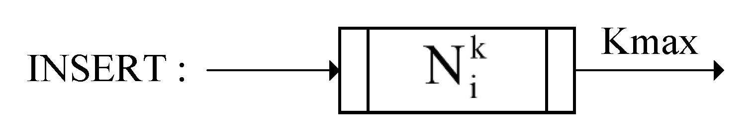
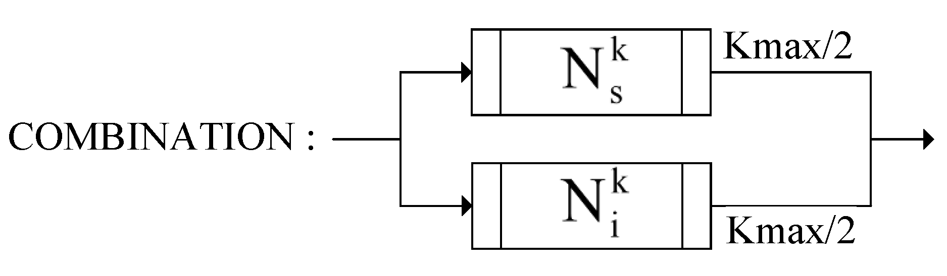
4.5.1. Neighborhood Structure Construction Operator

The improvement of the initial solution is implemented based on the neighborhood search algorithm, where the neighborhood structure is crucial for the algorithm’s search trajectory because it determines the topological properties of the search space. Generally, swapping and insertion are two basic operations of neighborhood search algorithms. In the workflow scenario studied in this paper, where tasks have complex partial order constraints, operations cannot be completely random insertions or swaps. Instead, they must be conducted under certain rules, and their execution processes are shown in Figure 2. The swap operation involves randomly selecting two tasks at the same depth and exchanging their positions to generate a new sequence of tasks. Meanwhile, the insertion operation involves randomly selecting and removing a task and then randomly choosing a position between its closest predecessor and successor to insert the task.   

Algorithm 1: Allocating Algorithm—EFT

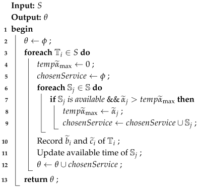
Algorithm 2: Allocating Algorithm—SET

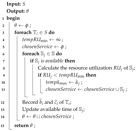
Algorithm 3: Allocating Algorithm—LRU

The insertion and swap operations can also be considered as two basic neighborhood structures, ${\mathcal{N}}_s$ and ${\mathcal{N}}_i$, respectively. Based on these two basic operations, this paper proposes three construction operators to create different neighborhoods, namely SWAP, INSERT, and COMBINATION.

SWAP generates a random swap neighborhood solution for the current solution ${\pi }_c$ by exchanging any $k(1\le k\le Kmax)$ pairs of tasks $\pi \left[i\right]$ and $\pi \left[j\right](0<i<j\le n)$ at the same depth. This process is repeated $Kmax$ times to obtain the swap neighborhood structure ${\mathcal{N}}_s^k\left({\pi }_c\right)$, which includes $Kmax$ random swap neighborhood solutions. An illustration of the SWAP construction operator is shown in Figure 3.

INSERT generates a random insertion neighborhood solution for the current solution ${\pi }_c$ by randomly selecting any $k(1\le k\le Kmax)$ tasks $\pi \left[i\right](0<i\le n)$ and inserting each $\pi \left[i\right]$ into any position between its closest predecessor and successor tasks. This process is repeated $Kmax$ times to obtain the insertion neighborhood structure ${\mathcal{N}}_i^k\left({\pi }_c\right)$, which includes $Kmax$ random insertion neighborhood solutions. An illustration of the INSERT construction operator is shown in Figure 4.

The COMBINATION operator, based on the current solution ${\pi }_c$ generates $Kmax/2$ random swap neighborhood solutions and $Kmax/2$ random insertion neighborhood solutions separately using the swap and insertion operators. In total, $Kmax$ neighborhood solutions are obtained to form the composite neighborhood structure of the current solution ${\pi }_c$. An illustration of the INSERT construction operator is shown in Figure 5.

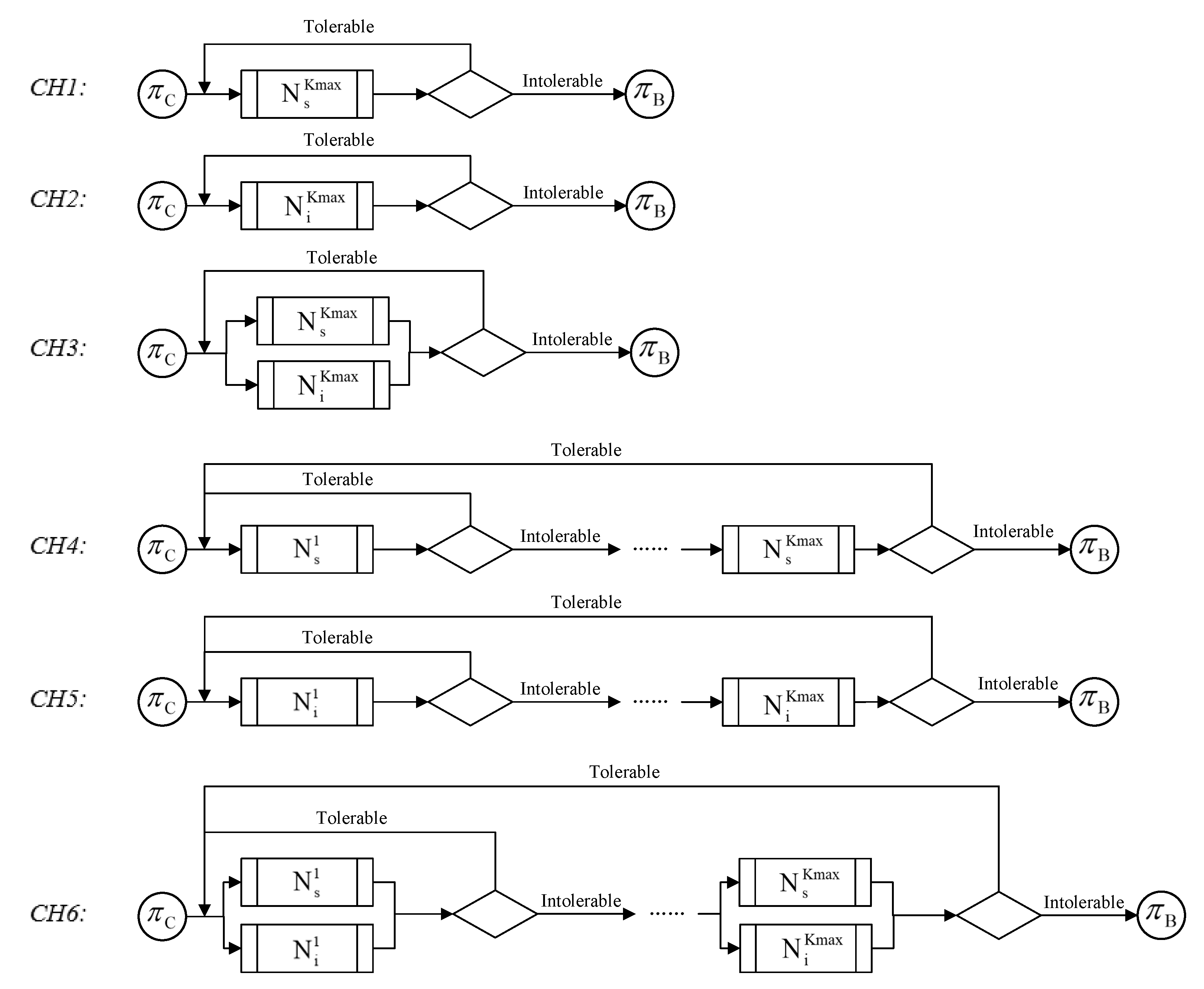
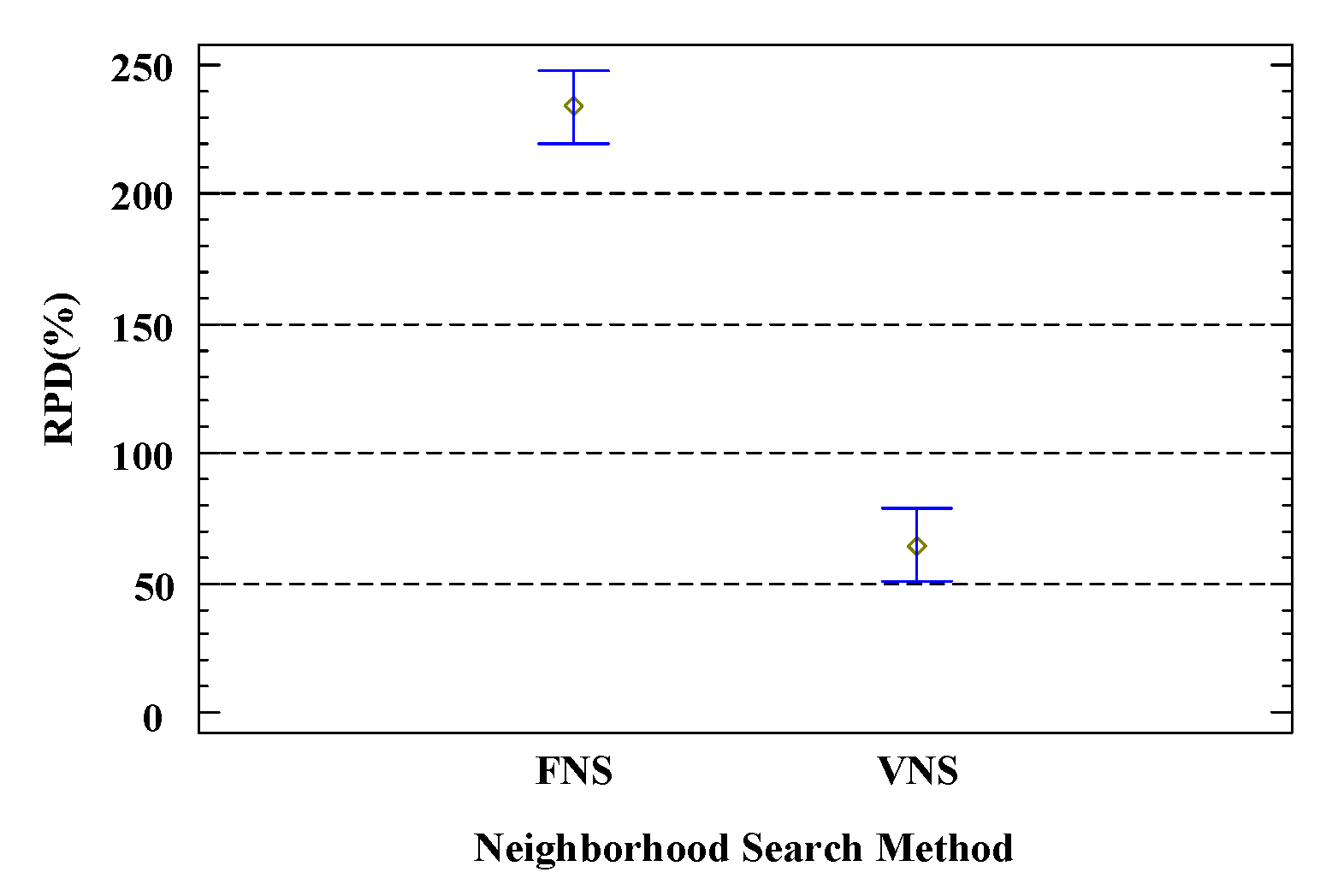
4.5.2. Neighborhood Search Method

Based on the aforementioned three construction operators, different neighborhoods can be generated for searching. Different search methods lead to different neighborhood transformation rules as well as limitations on the search for local optima and optimal solutions, resulting in different search trajectories and ultimately converging to different optimal solutions. In light of the characteristics of the research problem, this paper proposes two search methods: Fixed Neighborhood Search (FNS) and Variable Neighborhood Search (VNS), utilizing the operation count k to define the neighborhood transformation rules and the tolerance $\lambda$ to set the limits for searching local optima and optimal solutions.

FNS involves searching within a fixed neighborhood to find the optimal solution, where the value k is set to a constant $Kmax$. By performing $k=Kmax$ random operations using a certain construction operator, a random neighborhood solution is obtained. This process is repeated $Kmax$ times, ultimately yielding $Kmax$ neighborhood solutions to form the current solution ${\pi }_c$’s neighborhood, also known as the Candidate Restart Points Set ($CRPSet$). $CRPSet$ is then traversed; if a better solution is found, it is stored as the optimal solution, and the current tolerance value is reset to zero. Conversely, if no better solution is found after $\lambda$ consecutive attempts, the search is stopped, and the most recently recorded optimal solution is taken as the final optimal solution. The algorithm framework for Fixed Neighborhood Search is shown in Algorithm 4.

We will prove the total correction of Algorithm 4 in Theorem 1.

Theorem 1.

Algorithm 4 terminates within $\lceil \lambda /\delta \rceil$ iterations, where δ is the minimal delay improvement.

Algorithm 4: Fixed Neighborhood Search (FNS)

Proof. 

The proof proceeds in three steps:

1.

From Equation (35), we know the RPD (Relative Percentage Deviation) is monotonically decreasing, since each iteration only accepts improved solutions:

$${\mathrm{RPD}}^{(k+1)}\le {\mathrm{RPD}}^{\left(k\right)}$$

2.

Let $\delta =min\{\tilde{T}\left({\pi }_N\right)-\tilde{T}\left({\pi }_B\right)\}>0$, where this positive minimum is guaranteed by the discrete nature of fuzzy numbers.

3.

When the counter temp $\lambda$ accumulates $\lambda$ consecutive iterations without improvement, we must have:

$$\Delta \tilde{T}=\tilde{T}\left({\pi }_N\right)-\tilde{T}\left({\pi }_B\right)<\delta$$

which triggers loop termination by the algorithm’s stopping condition.

Therefore, the worst-case iteration count is bounded by the ceiling of $\lambda /\delta$.    □

VNS is to construct multiple different neighborhoods by choosing different values of $k\in \{1,2,\dots ,Kmax\}$ and to systematically search for these neighborhoods. The search begins in the smallest neighborhood ($k=1$), and when no improvement is made within the tolerance limit, the search moves to the next slightly larger neighborhood ($k=2$). For each neighborhood from $k=1$ to $Kmax$, CRPSet is generated using a certain construction operator, and this set is searched randomly within the tolerance limit. If a better solution is found to further improve the search, the search restarts from the smallest neighborhood with the better solution as the restart point; otherwise, the search continues to switch to larger neighborhoods based on the current solution, until the largest neighborhood is searched. The algorithm framework for Variable Neighborhood Search is shown in Algorithm 5.

Setting $\lambda =K_{\max }$ ensures full neighborhood exploration, with convergence guaranteed when $\Delta \tilde{T}<1\%$ over 10 consecutive iterations (see Theorem 1 for the formal proof).

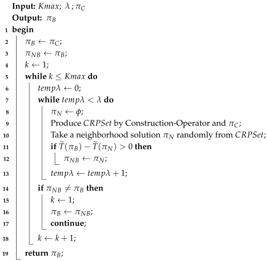
Algorithm 5: Variable Neighborhood Search (VNS)

4.5.3. Neighborhood Structure and Composite Heuristic Neighborhood Search Algorithm

The tolerance-aware composite heuristic neighborhood search further optimizes the scheduling scheme, deploying neighborhood structure construction operators to enhance the diversity of neighborhood solutions. It uses the value k to limit the size of the search space and introduces the concept of tolerance to ensure reasonable search boundaries. Based on the three neighborhood structure construction operators and the two neighborhood search methods proposed before, six composite neighborhood structures were constructed, and six corresponding composite heuristic neighborhood search methods $CHi(i=1,...,6)$ were developed. The schematic diagram of the six composite heuristic algorithms is shown in Figure 6.

$CH1$ is a composite form of the SWAP neighborhood construction operator and FNS, using the swap operator SWAP to construct the initial solution’s $k=Kmax$ random swap neighborhood. This neighborhood is a $CRPSet$ that contains $Kmax$ restart points. The current tolerance $temp\lambda$ is set to 0, and the initial solution ${\pi }_C$ is set as the best solution ${\pi }_B$. Without activating the tolerance limit $\lambda$, the search continues in the current neighborhood. If the total delay obtained from the current neighborhood solution as a scheduling scheme is lower than the best solution, then the current neighborhood solution is recorded as the best solution, the current tolerance is reset to zero, and the search continues; otherwise, the current tolerance is incremented by 1 and the search proceeds. This continues until the tolerance limit is triggered or the CRPSet is completely traversed. $CH2$ and $CH3$ are, respectively, composite forms of the INSERT and COMBINATION neighborhood construction operators with FNS. $CH2$ uses the insertion operator INSERT to construct the initial solution’s $k=Kmax$ random insertion neighborhood, while $CH3$ uses the composite operator COMBINATION to construct the initial solution’s $k=Kmax$ random composite neighborhood. The subsequent steps are similar to those in $CH1$.

$CH4$ is a composite form of the SWAP neighborhood construction operator and VNS, using the swap operator SWAP to construct the initial solution’s $k=1$ random swap neighborhood, which is a CRPSet containing $Kmax$ restart points. The current tolerance $temp\lambda$ is set to 0, and the initial solution ${\pi }_C$ is set as both the best solution ${\pi }_B$ and the best solution in the current neighborhood ${\pi }_{NB}$. Without activating the tolerance limit $\lambda$, the search continues in the current neighborhood. If the total delay obtained from the current neighborhood solution as a scheduling scheme is lower than the best solution, then the current neighborhood solution is recorded as the best in the current neighborhood and the current tolerance $temp\lambda$ is increased by 1 to continue the search; otherwise, only the current tolerance $temp\lambda$ is increased by 1 to continue the search. This continues until the tolerance limit is activated or the CRPSet is completely traversed, thus searching for the best current neighborhood solution from $\lambda$ neighborhood solutions. If the best solution in the current neighborhood is better than the best overall solution, then the best neighborhood solution is recorded as the best overall solution, and the search for $k=1,...,Kmax$ in the variable neighborhood restarts; if the best solution in the current neighborhood is not better than the best overall solution, then k is incremented by 1, and the search for the next k value neighborhood based on the original best solution continues until all $Kmax$ neighborhoods have been searched.

$CH5$ and $CH6$ are, respectively, composite forms of the INSERT and COMBINATION neighborhood construction operators with VNS. $CH5$ uses the insertion operator INSERT to construct solutions in the $k=1,...,Kmax$ random insertion neighborhood, while $CH6$ uses the composite operator COMBINATION to construct solutions in the $k=1,...,Kmax$ random composite neighborhood, with subsequent steps similar to those in $CH4$.

5. Experimental Results

In the proposed TANS algorithm framework, there are several variants of its components and parameters. We first calibrate these components and parameters and select the best combination to address the problem considered. Subsequently, the calibrated algorithm is compared with existing highly relevant algorithms in terms of effectiveness and robustness. All algorithms in the experiment are implemented in Java language and run on the same server configured with an Intel Xeon® Gold 6148 CPU @ 2.40 GHz × 80 with 256 GBytes of RAM. To verify the practical effectiveness of the TANS algorithm in fuzzy scheduling optimization scenarios, the required fuzzy uncertain information, such as the execution speed of services and the logistics cost arising from different geographical distributions between services, is randomly generated. The Analysis of Variance (ANOVA) technique is used to calibrate different components and parameters of the algorithm.

In experiments, the number of tasks contained in the workflow $n\in \{50,100,150,200,250\}$; to ensure the reasonableness of the deadlines, a deadline factor $ϵ\in \{1.0,1.1,1.2,1.3,1.4,1.5\}$ is set for the workflow to generate deadline constraints of varying urgency levels. The task workload follows a uniform distribution U (1, 30,000). For each combination of values for n and $ϵ$, 10 random instances are generated, resulting in a total of 300 random workflow instances. The number of service resources $m\in \{10,20,30,40,50\}$, the highest value of the fuzzy execution speed of services follows a uniform distribution U (500, 1000), and the highest value of the fuzzy logistics time between services follows a uniform distribution U (0, 10); on this basis, the min and max values are set based on the fuzzy fluctuation factor $e_{\tilde{x}}=0.1$. Detailed experimental parameters are shown in

Table 3. Experimental parameter settings.

Variable	Value
n	$\{50,100,150,200,250\}$
${\omega }_i$	U(1,30000)
$ϵ$	$\{1.0,1.1,1.2,1.3,1.4,1.5\}$
m	$\{10,20,30,40,50\}$
${\tilde{\alpha }}_i^{\mathrm{most}}$	U(500,1000)
${\tilde{l}}_{i,j}^{\mathbb{S}\mathrm{most}}$	U(0,10)
${\tilde{l}}_{i,i}^{\mathbb{S}\mathrm{most}}$	0
$e_{\tilde{x}}$	0.1

.

This experiment uses the Relative Percentage Deviation (RPD) as the algorithm evaluation metric, with the calculation equation as follows:

$$\begin{array}{c}RPD(\%)={\displaystyle \frac{\tilde{T}\left({\pi }_C\right)-\tilde{T}\left({\pi }_B\right)}{\tilde{T}\left({\pi }_B\right)}}\times 100\%\end{array}$$

(35)

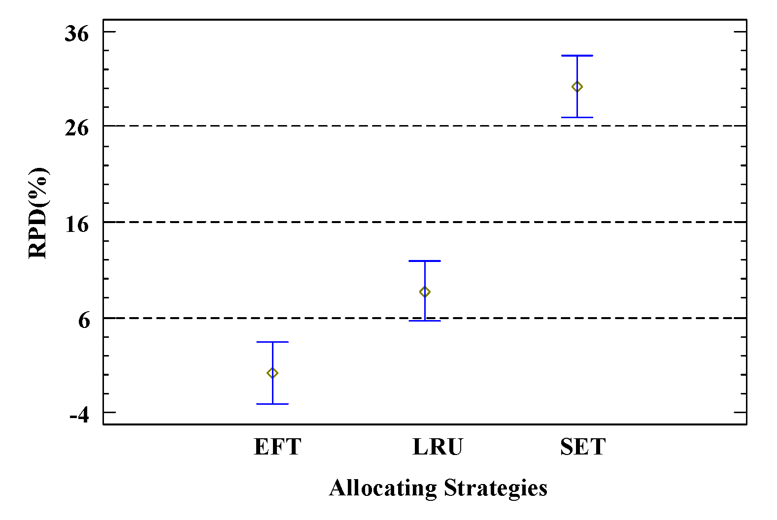
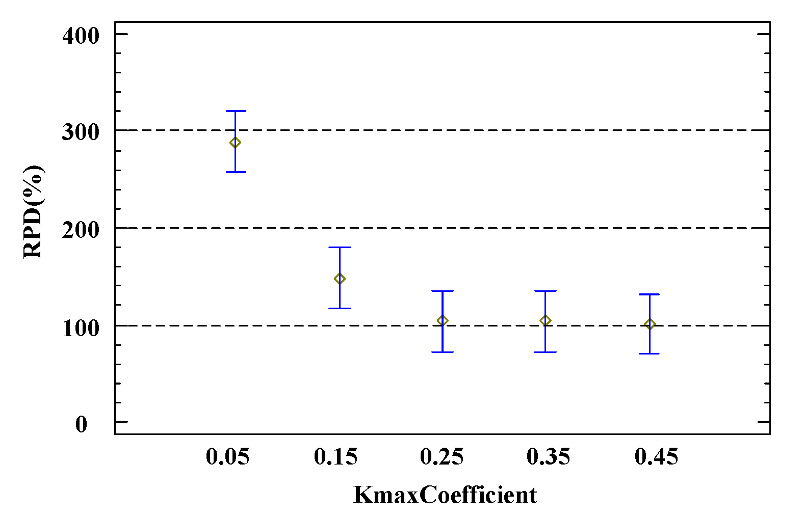
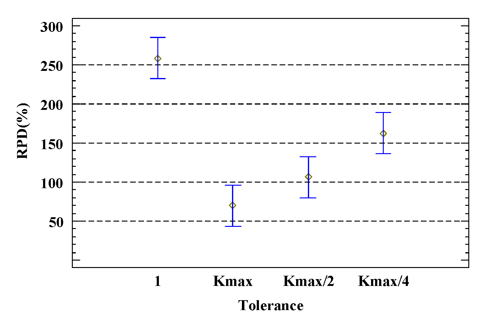
5.1. Parameter and Component Calibration

The calibration of the components and parameters in this paper is divided into two parts, with all experiments conducted under the 95% Tukey HSD confidence interval. Error bars represent 95% confidence intervals; all pairwise comparisons show statistically significant differences ($p<0.01$, Tukey’s hsd test). In the initial solution generation part, involved components include the RSDS and TSDS from the task fuzzy sub-deadline partitioning component, and the RFSD, TFSD, SWFT from the task scheduling sequence generation component (where RFSD and TFSD are implementations based on two strategies of task fuzzy sub-deadline partitioning), and the EFT, SET, LRU from the service search and matching component. Based on the above combinations, 3 × 3 = 9 combination schemes are constructed, and combined with the settings for workflow instances and service resource states, a total of 300 × 5 × 9 = 13,500 experiments are conducted.

Figure 7 presents the comparison results corresponding to different task scheduling sequence generation strategies. It is noteworthy that since the two strategies of task fuzzy sub-deadline partitioning correspond one-to-one with RFSD and TFSD in task scheduling sequence generation, the strategy selection during the task scheduling sequence generation phase includes the choice of sub-deadline partitioning strategy. Figure 7 shows that SWFT significantly outperforms RFSD and TFSD. A possible reason is that RFSD and TFSD strategies only focus on the sub-deadline of individual tasks, whereas SWFT takes into account both the execution and logistics of the current task and all successor tasks, which is more conducive to optimizing the total delay. Based on the analysis above, SWFT is chosen as the strategy for the task scheduling sequence generation component.

Figure 8 shows the results of different search and matching strategies of services. The RPD value of EFT is close to 0, LRU fluctuates between 5 and 14, and SET fluctuates between 26 and 36, with EFT clearly performing better. Although EFT does not directly consider balancing the utilization rate of different service resources compared to LRU, it selects from idle service resources without causing significant congestion. Additionally, compared to SET, EFT considers the impact of logistics time on total delay on top of execution time. Therefore, EFT is chosen as the strategy for the search and matching component of the service.

In the neighborhood search part, this paper proposes six composite heuristic neighborhood search methods composed of three neighborhood structure construction operators and two neighborhood search methods. The components involved include SWAP, INSERT, and COMBINATION from the neighborhood structure construction operator component and FNS and VNS from the neighborhood search methods. The calibration parameters include five values for the maximum neighborhood structure number coefficient $Kma{x}^{Cofficient}$ and four values for the tolerance $\lambda$. Thus, there are a total of 3 × 2 × 5 × 4 = 120 strategy combination schemes. Combined with the settings for workflow instances and service resource states, a total of 300 × 5 × 120 = 180,000 experiments are conducted.

Figure 9 shows the impact of different neighborhood structure construction operators on the total delay of workflows. From the figure, it is observed that COMBINATION performs best, with an RPD 50% lower than INSERT and 75% lower than SWAP. Figure 10 displays the impact of different neighborhood search methods on the total delay of workflows. Among them, VNS significantly outperforms FNS, likely because VNS has a much larger search space than FNS, which can enhance the quality of the global optimal solution. Figure 11 shows the impact of different values for the maximum neighborhood structure number coefficient. From the figure, it is evident that as $Kma{x}^{Cofficient}$ increases, the RPD value shows a downward trend until it stabilizes. Figure 12 presents the impact of different tolerance values. The lowest RPD value occurs when $\lambda =Kmax$. According to the definition of neighborhood structure, when $\lambda =Kmax$, all candidate neighborhood solutions are traversed, ultimately enhancing the quality of the optimization scheme.

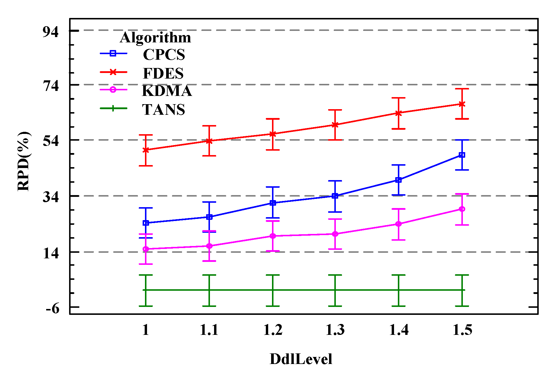
5.2. Algorithm Evaluation

This paper compares the proposed TANS algorithm with three similar existing works, KDMA [22], CPCS [27], and FDES [28].

• Baseline 1 (KDMA): KDMA is a memetic workflow scheduling algorithm that embeds a heuristic local search operator into the metaheuristic algorithm to combine their strengths and complement each other’s shortcomings.
• Baseline 2 (CPCS): CPCS is a scheduling algorithm that clusters tasks using a recursive critical path. Since list scheduling and clustering scheduling represent two categories within heuristic scheduling, comparing CPCS with the list scheduling algorithm proposed in this paper is of significant importance.
• Baseline 3 (FDES): FDES is a fuzzy dynamic event scheduling algorithm based on heap sorting. Comparing it with the static scheduling scheme generated by the algorithm proposed in this paper can provide a more comprehensive validation of the performance of our algorithm.

In addition, in conjunction with the settings for the workflow instances and the service resource states, a total of 3000 × 5 × 4 = 6000 experiments will be conducted. To evaluate the statistical robustness of the proposed TANS method, we employed an Analysis of Variance (ANOVA) test across multiple simulation runs for each configuration. The ANOVA analysis inherently captures the statistical error and variability of the results, reflecting the consistency and reliability of the scheduling outcomes. Our evaluation showed statistically significant improvements of TANS over baseline methods (KDMA, CPCS, FDES) with p-values consistently less than 0.05, demonstrating robust performance across diverse cloud manufacturing scenarios.

Figure 13 shows the results of the comparison of the RPD values for the total delay of the workflows under different task quantities for four algorithms within the 95% Tukey HSD confidence interval. Across various workflow task sizes, the TANS algorithm proposed in this chapter consistently outperforms the other comparative algorithms. The performance of the KDMA and CPCS algorithms varies with the number of tasks. FDES performs the worst due to its lack of consideration for a global strategy. When $n<170$, the RPD values for KDMA are lower than those for CPCS; when $n>170$, the RPD values for CPCS are lower than those for KDMA. This is because with fewer tasks, the workflow structure is simpler, and the clustering scale is smaller and less effective, showing no advantage over the list scheduling algorithm KDMA. As the number of tasks increases, the workflow topology becomes more complex and the scale of tasks included in the critical path increases. At this point, using a clustering algorithm that can map all tasks on the critical path to the fastest service resource en masse without considering the logistics process performs better. Overall, the optimization effect of TANS is significant, outperforming the other three algorithms in terms of total workflow delay in any task size scenario.

Figure 14 shows the results of the comparison of the RPD values for the total delay of the workflows under different numbers of service resources for four algorithms within the confidence interval 95% Tukey HSD. Under various quantities of service resources, the KDMA proposed in this chapter consistently outperforms the three comparative algorithms. The RPD values for FDES are always higher than those for the other three algorithms, maintaining a generally flat trend with a slight decrease in fluctuation at $m=20$. The inferior performance of FDES may be due to its scheduling approach, which only focuses on the current ready-to-schedule tasks without considering the priority sequence of all tasks included in the workflow from a global perspective, leading to sub-par performance in static scheduling. TANS shows the most significant advantage over the other three, with its RPD values on average 24% lower than KDMA, 32% lower than CPCS, and 60% lower than FDES. Therefore, it is evident that under different scenarios of quantity of service resources, the TANS algorithm proposed in this chapter performs the best, capable of reducing total workflow delay by an average of approximately 39% compared to other comparative algorithms.

Figure 15 shows the results of the comparison of the RPD values for the total delay of the workflows under different deadline factors for four algorithms within the 95% Tukey HSD confidence interval. As the deadline factor $ϵ$ increases, the RPD values of KDMA, CPCS, and FDES all show an upward trend. When $ϵ=1.5$, the RPD values of KDMA, CPCS, and FDES reach their maximum at 22%, 50%, and 64%, respectively. From the analysis above, it is evident that with changes in the deadline factor, either under tight or relaxed workflow deadline constraints, TANS shows better results compared to the other three algorithms, effectively reducing the total workflow delay by an average of 35%. Furthermore, when the deadline is tight, that is, $ϵ=1$, the total delay of the optimized scheduling scheme provided by TANS is approximately 14% lower than that of the initial scheduling scheme; when the deadline is more relaxed, that is, $ϵ=1.5$, it is about 22%.

6. Conclusions

In this study, we presented the Tolerance-Aware Neighborhood Search (TANS) method for workflow scheduling with fuzzy uncertainties in cloud manufacturing environments. Extensive experiments demonstrated that TANS achieves significant improvements over classical scheduling methods (KDMA, CPCS, and FDES) in terms of key performance metrics. Specifically, TANS reduced the average Relative Percentage Deviation (RPD) of lateness by 38.7% compared to CPCS and 42.1% compared to FDES. These results confirm the effectiveness of TANS in handling fuzzy uncertainties and optimizing both time efficiency and logistics expenditures in distributed manufacturing networks.

Despite these promising results, certain limitations remain. First, the current implementation assumes deterministic logistics costs, which may not fully capture real-world cost fluctuations. Second, energy consumption is not explicitly considered in the optimization process, which could be an important factor in sustainable manufacturing. Lastly, the majority of the experimental evaluation was conducted on synthetic datasets, which, although comprehensive, may not fully reflect real-world manufacturing complexities. Addressing these limitations could further enhance the robustness and applicability of the proposed method.

For future work, we plan to extend the evaluation to real-world datasets and integrate energy-aware scheduling strategies in addition to incorporating real-time adaptive mechanisms. We also suggest exploring multi-objective optimization techniques to balance time efficiency, logistics costs, and energy consumption in large-scale cloud manufacturing environments.

References

1. Li, F.; Liao, W.; Cai, W.; Zhang, L. Multitask Scheduling in Consideration of Fuzzy Uncertainty of Multiple Criteria in Service-Oriented Manufacturing. IEEE Trans. Fuzzy Syst. 2020, 28, 2759–2771. [Google Scholar] [CrossRef]
2. Zhu, G.; Shao, X. A Scheduling Optimization Algorithm Based on Non-Cooperative Game in the Cloud Manufacturing. In Proceedings of the 2022 8th International Conference on Information Management (ICIM), Cambridge, UK, 25–27 March 2022; pp. 155–159. [Google Scholar] [CrossRef]
3. Ma, Y.; Xu, W.; Tian, S.; Liu, J.; Zhou, Z.; Hu, Y.; Feng, H. Digital Twin Enhanced Optimization of Manufacturing Service Scheduling for Industrial Cloud Robotics. In Proceedings of the 2020 IEEE 18th International Conference on Industrial Informatics (INDIN), Warwick, UK, 20–23 July 2020; Volume 1, pp. 469–476. [Google Scholar] [CrossRef]
4. Li, X.; Wang, X.; Zhao, Y.; Dong, Y.; Wang, P. Improved Grey Wolf Optimization Algorithm for Solving Cloud Manufacturing Scheduling Problem with Limit Logistics Resource. In Proceedings of the 2021 4th International Conference on Artificial Intelligence and Big Data (ICAIBD), Chengdu, China, 28–31 May 2021; pp. 174–178. [Google Scholar] [CrossRef]
5. Bi, X.; Yu, D.; Liu, J.; Hu, Y. Multi-Agent Scheduling System in Cloud Manufacturing Environment. In Proceedings of the 2020 10th Institute of Electrical and Electronics Engineers International Conference on Cyber Technology in Automation, Control, and Intelligent Systems (CYBER), Xi’an, China, 10–14 October 2020; pp. 385–389. [Google Scholar]
6. Zhang, Y.; Yu, J. Research on High-Efficiency Resource Allocation of Multi-edge Devices Based on Cloud Manufacturing Mode. In Proceedings of the 2021 IEEE International Conference on Power, Intelligent Computing and Systems (ICPICS), Shenyang, China, 29–31 July 2021; pp. 682–687. [Google Scholar] [CrossRef]
7. Liu, S.; Li, L.; Zhang, L.; Shen, W. Game Theory Based Dynamic Event-Driven Service Scheduling in Cloud Manufacturing. IEEE Trans. Autom. Sci. Eng. 2022, 21, 618–629. [Google Scholar] [CrossRef]
8. Zhang, L.; Yang, C.; Yan, Y.; Hu, Y. Distributed Real-Time Scheduling in Cloud Manufacturing by Deep Reinforcement Learning. IEEE Trans. Ind. Inform. 2022, 18, 8999–9007. [Google Scholar] [CrossRef]
9. Yang, F.; Feng, T.; Xu, F.; Jiang, H.; Zhao, C. Collaborative clustering parallel reinforcement learning for edge-cloud digital twins manufacturing system. China Commun. 2022, 19, 138–148. [Google Scholar] [CrossRef]
10. Lin, B.; Lin, C.; Chen, X.; Lin, M.; Huang, G.; Xu, Z. Cost-Driven Scheduling for Workflow Decision Making Systems in Fuzzy Edge-Cloud Environments. IEEE Trans. Autom. Sci. Eng. 2025, 22, 3756–3771. [Google Scholar] [CrossRef]
11. Yang, Y.; Shen, H.; Tian, H. Scheduling Workflow Tasks With Unknown Task Execution Time by Combining Machine-Learning and Greedy-Optimization. IEEE Trans. Serv. Comput. 2024, 17, 1181–1195. [Google Scholar] [CrossRef]
12. Rajput, K.Y.; Li, X.; Zhang, J.; Lakhan, A. A Novel Scheduling Approach for Spark Workflow Tasks With Deadline and Uncertain Performance in Multi-Cloud Networks. IEEE Trans. Cloud Comput. 2024, 12, 1145–1157. [Google Scholar] [CrossRef]
13. Wang, Y.J.; Wang, G.G.; Tian, F.M.; Gong, D.W.; Pedrycz, W. Solving energy-efficient fuzzy hybrid flow-shop scheduling problem at a variable machine speed using an extended NSGA-II. Eng. Appl. Artif. Intell. 2023, 121, 105977. [Google Scholar] [CrossRef]
14. Sun, M.; Cai, Z.; Zhang, H. A teaching-learning-based optimization with feedback for L-R fuzzy flexible assembly job shop scheduling problem with batch splitting. Expert Syst. Appl. 2023, 224, 120043. [Google Scholar] [CrossRef]
15. Zhou, W.; Chen, F.; Ji, X.; Li, H.; Zhou, J. A Pareto-based discrete particle swarm optimization for parallel casting workshop scheduling problem with fuzzy processing time. Knowl.-Based Syst. 2022, 256, 109872. [Google Scholar] [CrossRef]
16. Zhang, Y.; Liu, J. Emergency Logistics Scheduling Under Uncertain Transportation Time Using Online Optimization Methods. IEEE Access 2021, 9, 36995–37010. [Google Scholar] [CrossRef]
17. Congcong, C.; Yueyu, L.; Jiaojiao, W. A Dynamic Optimization Method of Intelligent Material Distribution Based on Hybrid Heuristic Algorithm. In Proceedings of the 2020 9th International Conference on Industrial Technology and Management (ICITM), Oxford, UK, 11 February 2020; pp. 210–214. [Google Scholar]
18. Fizza, K.; Auluck, N.; Azim, A. Improving the Schedulability of Real-Time Tasks Using Fog Computing. IEEE Trans. Serv. Comput. 2022, 15, 372–385. [Google Scholar] [CrossRef]
19. Mukherjee, M.; Kumar, V.; Zhang, Q.; Mavromoustakis, C.X.; Matam, R. Optimal Pricing for Offloaded Hard- and Soft-Deadline Tasks in Edge Computing. IEEE Trans. Intell. Transp. Syst. 2022, 23, 9829–9839. [Google Scholar] [CrossRef]
20. He, X.; Dou, W. Offloading Deadline-aware Task in Edge Computing. In Proceedings of the 2020 IEEE 13th International Conference on Cloud Computing (CLOUD), Beijing, China, 18–24 October 2020; pp. 28–30. [Google Scholar] [CrossRef]
21. He, X.; Zheng, J.; He, Q.; Dai, H.; Liu, B.; Dou, W.; Chen, G. CONFECT: Computation Offloading for Tasks with Hard/Soft Deadlines in Edge Computing. In Proceedings of the 2021 IEEE International Conference on Web Services (ICWS), Chicago, IL, USA, 5–10 September 2021; pp. 262–271. [Google Scholar] [CrossRef]
22. Yao, F.; Chen, H.; Liu, X.; Gong, M.; Xing, L.; Zhao, W.; Zheng, L. A Multi-Objective Memetic Algorithm for Workflow Scheduling in Clouds. IEEE Trans. Emerg. Top. Comput. Intell. 2024. [Google Scholar] [CrossRef]
23. Cai, K.; Wu, Q.; Zhou, M.; Chen, C.; Wen, J.; Wang, S. Dynamically Scheduling Deadline-Constrained Interleaved Workflows on Heterogeneous Computing Systems. IEEE Trans. Serv. Comput. 2025, 18, 758–769. [Google Scholar] [CrossRef]
24. Nakahira, Y.; Ferragut, A.; Wierman, A. Generalized Exact Scheduling: A Minimal-Variance Distributed Deadline Scheduler. Oper. Res. 2020, 71, 397–790. [Google Scholar] [CrossRef]
25. ISO 22400:2014; Automation Systems and Integration—Key Performance Indicators (KPIs) for Manufacturing Operations Management. International Organization for Standardization: Geneva, Switzerland, 2014.
26. IEEE Std 1855-2016; IEEE Standard for Fuzzy Markup Language. IEEE: New York, NY, USA, 2016.
27. Ebaid, A.; Ammar, R.; Rajasekaran, S.; Fergany, T. Task clustering & scheduling with duplication using recursive critical path approach (RCPA). In Proceedings of the 10th IEEE International Symposium on Signal Processing and Information Technology, Luxor, Egypt, 15–18 December 2010; pp. 34–41. [Google Scholar] [CrossRef]
28. Zhu, J.; Li, X.; Ruiz, R.; Li, W.; Huang, H.; Zomaya, A.Y. Scheduling Periodical Multi-Stage Jobs With Fuzziness to Elastic Cloud Resources. IEEE Trans. Parallel Distrib. Syst. 2020, 31, 2819–2833. [Google Scholar] [CrossRef]
Figure 1. Framework of workflow scheduling in cloud manufacturing.
Mathematics 13 01806 g001
Figure 2. Execution process of the two basic operations.
Mathematics 13 01806 g002
Figure 3. Illustration of SWAP.
Mathematics 13 01806 g003
Figure 4. Illustration of INSERT.
Mathematics 13 01806 g004
Figure 5. Illustration of COMBINATION.
Mathematics 13 01806 g005
Figure 6. Schematic diagram of the composite heuristic algorithm C H i i = 1 , , 6 .
Mathematics 13 01806 g006
Figure 7. Sequencing strategies under 95% Tukey HSD confidence interval.
Mathematics 13 01806 g007
Figure 8. Allocating strategies under 95% Tukey HSD confidence interval.
Mathematics 13 01806 g008
Figure 9. Construction operators under 95% Tukey HSD confidence interval.
Mathematics 13 01806 g009
Figure 10. Neighborhood search method under 95% Tukey HSD confidence interval.
Mathematics 13 01806 g010
Figure 11. K max coefficient under 95% Tukey HSD confidence interval.
Mathematics 13 01806 g011
Figure 12. Tolerance λ under 95% Tukey HSD confidence interval.
Mathematics 13 01806 g012
Figure 13. Impact of different task number under 95% Tukey HSD confidence interval.
Mathematics 13 01806 g013
Figure 14. Impact of different resource number under 95% Tukey HSD confidence interval.
Mathematics 13 01806 g014
Figure 15. Impact of different deadline factors under 95% Tukey HSD confidence interval.
Mathematics 13 01806 g015