Abstract
Large-scale crowd flow prediction is a critical task in urban management and public safety. However, achieving accurate and efficient prediction remains challenging. Most existing models overlook spatial heterogeneity, employing unified parameters to fit diverse crowd flow patterns across different spatial units, which limits their accuracy. Meanwhile, the massive spatial units significantly increase the computational cost, limiting model efficiency. To address these limitations, we propose a novel model for large-scale crowd flow prediction, namely the Stratified Compressive Sensing Network (SCS-Net). First, we develop a spatially stratified module that posterior adaptively extracts the underlying spatially stratified structure, effectively modeling spatial heterogeneity. Then, we develop compressive sensing modules to compress redundant information from massive spatial units and learn shared crowd flow patterns, enabling efficient prediction. Finally, we conduct experiments on a large-scale real-world dataset. The results demonstrate that SCS-Net outperforms deep learning baseline models by 35.25–139.2% in MAE and 26.3–112.4% in RMSE while reducing GFLOPs by 53–1067 times and shortening training time by 3.1–83.2 times compared to prevalent spatio-temporal prediction models. Moreover, the spatially stratified structure extracted by SCS-Net offers valuable interpretability for spatial heterogeneity in crowd flow patterns, providing deeper insights into urban functional layouts.
Keywords:
crowd flow prediction; large scale; compressive sensing; spatial heterogeneity; spatially stratified structure MSC:
68T09
1. Introduction
With the accelerated pace of urbanization, urban population density has increased rapidly [1,2]. The improper allocation of urban infrastructure has triggered numerous issues, such as traffic congestion and crowd crush [3,4,5]. Crowd flow prediction, which aims to forecast the future total number of people entering or leaving a given region (i.e., inflows and outflows) [6,7,8], plays a crucial role in mitigating these issues. Specifically, accurate crowd flow predictions enable transportation authorities to dynamically adjust public transit resources and optimize urban infrastructure allocation. In addition, by providing early warnings of high crowd concentrations, these predictions support precautionary measures for urban public safety.
Temporal and spatial dependencies are fundamental for ensuring the predictability of crowd flow [9,10]. Since deep learning techniques have achieved significant progress in spatio-temporal prediction tasks, numerous recent studies have developed diverse neural network models to capture these dependencies [11,12]. Regarding spatial modeling, prevailing approaches are typically categorized into Convolutional Neural Network (CNN)-based models, Graph Neural Network-(GNN) based models, and attention-based models [13]. Although these methods effectively model spatio-temporal dependencies, the increasing demand for large-scale crowd flow prediction presents two major challenges: inaccuracy and inefficiency.
Firstly, inaccuracy is primarily attributable to spatial heterogeneity, which implies that spatio-temporal dependencies vary across different spatial units [14]. Existing crowd flow prediction models often overlook the influence of spatial heterogeneity. They employ unified parameters to fit the diverse crowd flow patterns across various spatial units, leading to unsatisfactory predictions [15]. Since the spatio-temporal evolution of crowd flow is closely related to human activities and regional functions [16,17], the patterns across different spatial units are not entirely unique but share certain similarities [18]. For example, workers typically commute daily between their residences and workplaces, while older adults often travel between parks and their homes during the day [19]. This regularity indicates that crowd flow patterns exhibit a spatially stratified structure, which categorizes the spatial units. Spatial units of the same type tend to display similar patterns. Since spatial heterogeneity becomes more significant at larger scales, it is crucial to understand and leverage this structure for effective modeling of spatial heterogeneity.
Secondly, inefficiency arises from the massive spatial units. Since existing crowd flow prediction models are primarily designed based on small-scale public datasets, the efficiency challenges introduced by large-scale prediction have not been adequately considered [20,21,22]. Specifically, due to irregular urban boundaries, CNN-based models struggle to be directly applied. A large number of unnecessary spatial units must be incorporated to fill the standardized tensor structures required for convolutional operations, leading to additional computational overhead and increased data noise. Although GNN-based and attention-based models can more flexibly adapt to diverse spatial unit distributions, their computational cost increases significantly with the expansion of spatial extent. When the number of spatial units grows by a factor of , the computational cost of the adjacency matrix and self-attention mechanism increases by a factor of , significantly reducing model efficiency. This highlights the urgent need for a more scalable and efficient model for large-scale crowd flow prediction.
In this study, we propose a novel model for large-scale crowd flow prediction, namely the Stratified Compressive Sensing Network (SCS-Net). The proposed SCS-Net consists of two key components: (1) a Spatially Stratified Module (SS-Module), which extracts the spatially stratified structure of crowd flow, and (2) several Compressive Sensing Modules (CS-Modules), which learn the shared crowd flow patterns. The main contributions of this study are summarized as follows:
- We developed a spatially stratified module to model spatial heterogeneity. This module enables posterior adaptive extraction of the spatially stratified structure from geographical environments, improving prediction accuracy.
- We developed several compressive sensing modules to enhance efficiency. By compressing redundant information among spatial units of the same type, this module facilitates the learning of shared crowd flow patterns, thereby significantly improving computational efficiency. Meanwhile, by leveraging the information lost after reconstruction, this module captures residual fluctuation patterns, further enhancing the model’s predictive capabilities.
- We evaluated our proposed model for large-scale crowd flow prediction in Fuzhou, China. Experimental results demonstrated its significant advantages over baseline models in both accuracy and efficiency. Based on the interpretability analysis of the spatially stratified structure, we found that spatial heterogeneity in crowd flow patterns is closely related to the urban functional layouts in Fuzhou.
2. Related Works
Crowd flow prediction has emerged as a pivotal task in urban dynamic monitoring, aiming to uncover spatio-temporal patterns from historical crowd flow data to forecast future crowd movements. It provides essential decision support for urban management and public safety. Hoang et al. (2016) proposed the first model for Forecasting Citywide Crowd Flow (FCCF) [6]. It leverages Intrinsic Gaussian Markov Random Fields to capture seasonal and trend components in crowd flow while employing a spatio-temporal residual model to learn spatio-temporal dependencies. Since then, driven by the strong capacity of neural network architectures to model these dependencies, numerous deep learning-based approaches have been developed [23]. Based on their spatial modeling strategies, these crowd flow prediction models can be broadly classified into CNN, GNN, and attention-based models.
CNN-based models, the most prevalent in crowd flow prediction, leverage convolutional operations to capture spatio-temporal dependencies in crowd flow data. For instance, the deep-learning-based prediction model for spatio-temporal data (DeepST) [24] and Spatio-Temporal Residual Network (ST-ResNet) [7] employ 2D convolutions to model spatial dependencies, as well as temporal closeness, periodicity, and trends. Building on this, Zheng et al. (2019) introduced 3D convolutions to enhance the modeling of spatio-temporal dependencies [25]. Since crowd flow patterns are constrained by the local receptive fields of standard convolutions, several improvements have been proposed. In the spatial domain, the ConvPlus architecture expands the spatial receptive field of convolutions [26,27]. In the temporal domain, recurrent neural networks (RNNs) have been combined with convolutional structures to extend the temporal receptive field [28,29,30,31]. However, due to the inherent limitation of convolutional operations on regular grid-based data, CNN-based models struggle to adapt to complex study areas with irregularly shaped spatial units.
GNN-based models can more flexibly handle complex spatial units, such as administrative districts [32]. For spatial modeling, existing studies primarily construct graphs based on spatial proximity, road connectivity, and functional similarity to capture spatial dependencies between units [17,33,34]. Based on this, the Graph Attention Network (GAT) has been introduced to enhance GNN-based models by adaptively assigning edge weights [35]. However, defining a suitable graph is challenging, as it often relies on prior knowledge.
Attention-based models apply self-attention mechanisms to adaptively learn the intrinsic spatio-temporal structures in crowd flow data [36,37]. To better capture the influence of the geographical environments, environmental factors are also mapped into embedding vectors and integrated into the spatio-temporal attention mechanism [38,39]. However, attention-based models frequently compute pairwise attention scores between spatial units, which is considerably less efficient compared to CNN-based and GNN-based models.
Meanwhile, most of these models are designed based on small-scale datasets, such as the TaxiNYC dataset (with 10 × 20 = 200 grids) and the BikeNYC dataset (with 16 × 8 = 128 grids). Since large-scale crowd flow prediction has become a critical demand in urban dynamic monitoring [40,41], these models overlook the impact of the number of spatial units on efficiency, making them difficult to apply in practice. Specifically, spatial convolutions often require numerous additional spatial units to maintain grid regularity, while the computational cost of graph convolutions and self-attention mechanisms increases significantly with the number of spatial units. Although Jiang et al. (2021) and Su et al. (2023) introduced pyramid structures to model the multi-scale spatio-temporal dependencies of large-scale crowd flow [20,42], the efficiency of these models remains concerning.
Moreover, these models overlook the impact of spatial heterogeneity, which limits their predictive performance. Since spatial units with similar geographical environments exhibit similar patterns [43], identifying the spatially stratified structure of spatial units has become an effective approach for modeling spatial heterogeneity [44,45]. Lin et al. (2023) applied K-shape clustering to extract spatial units of the same type for spatial heterogeneity modeling [19]. However, this method is constrained by its reliance on a priori linear similarity metrics. Liang et al. (2021) proposed an unsupervised Mincut loss to posteriorly cluster spatial units [15]. However, the loss enforces spatially compact and balanced clusters, which contradicts the irregular urban functional layouts and impairs interpretability. Therefore, accurately extracting the spatially stratified structure by incorporating geographical environments is crucial for enhancing the accuracy of crowd flow prediction models.
3. Preliminaries
Definition 1 (Spatial unit).
The fundamental units that constitute the study area. The most common shape of a spatial unit is a grid.
Definition 2 (Crowd flow).
The total number of people entering or leaving a spatial unit within a given time interval, including inflow and outflow. The crowd flow at time is denoted as , where denotes the number of spatial units.
Definition 3 (Geographical environments).
External factors related to crowd flow that characterize human activities, functions, and other attributes of spatial units. The geographical environments of the study area are represented as , where denotes the number of external factors.
Definition 4 (Large-scale area).
A study area is defined as large-scale if it comprises more than 10,000 spatial units or covers at least one entire city. This definition is empirically based on (i) the typical spatial resolution (1 km × 1 km) adopted in publicly available crowd flow datasets, (ii) the area of most cities, and (iii) the application contexts of large-scale crowd flow prediction. This empirical definition provides an explicit and testable reference for distinguishing between large-scale and small-scale crowd flow prediction.
Problem 1.
Here, we define the problem of large-scale crowd flow prediction as follows: Given historical crowd flow for spatial units during the time period from to , along with the geographical environments , the goal is to predict the future crowd flow for the time period from to .
4. Methodology
Figure 1 illustrates the framework of the proposed SCS-Net, which consists of a Spatially Stratified Module (SS-Module) and several Compressive Sensing Modules (CS-Modules). The SS-Module first clusters the spatial units based on their geographical environments to extract the spatially stratified structure. Then, for the spatial units in each cluster, a certain CS-Module compresses the redundant information in the historical crowd flow of the spatial units for efficient prediction. Finally, the parameters of SCS-Net are optimized through the prediction loss, the clustering loss, and the compressive sensing loss. We then aggregate the predictions of spatial units in different clusters to obtain the future crowd flow.
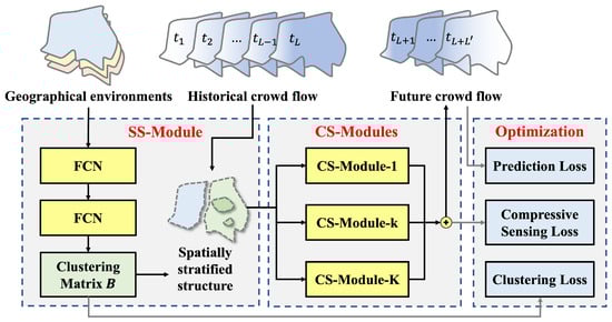
Figure 1.
Framework of the proposed SCS-Net.
4.1. Spatially Stratified Module
The influence of spatial heterogeneity on crowd flow is reflected in a certain spatially stratified structure, which is closely related to geographical environments. In other words, spatial units with similar geographical environments are likely to exhibit similar crowd flow patterns. Clustering the spatial units has been proven to be a feasible approach for extracting the spatially stratified structure. However, the results of prior clustering methods are often overly generic, as they are not customized for the crowd flow prediction task.
Therefore, we integrate the process of clustering spatial units into the neural network to capture the task-specific spatially stratified structure posteriorly. Specifically, we employ two fully connected neural networks to learn the correlations between different spatial units from the geographical environments . Based on this non-linear similarity measure, the clustering matrix can be obtained. The SS-Module can be formulated by the following equation:
where denotes the clustering matrix, and denotes the number of clusters. Each column of represents the probabilities of all spatial units belonging to a specific cluster; each row of corresponds to the classification vector of a spatial unit, representing its probabilities of belonging to each cluster. Spatial units with more similar geographical environments will have more similar classification vectors. denotes the ReLU activation function; denotes the Softmax activation function; , , and are all learnable parameters.
4.2. Compressive Sensing Module
In large-scale crowd flow prediction, existing CNN, GNN, and attention-based models are all constrained by the computational cost of spatial modeling. To address this, we introduce the idea of compressive sensing from the signal processing field. Compressive sensing extracts key information in the sparse domain (e.g., frequency-domain signals) from discrete sampling signals, enabling efficient reconstruction of the original signal. In crowd flow, such key information corresponds to the shared patterns. We develop a flexible and efficient prediction architecture with linear complexity, namely the CS-Module, as illustrated in Figure 2.
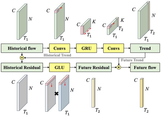
Figure 2.
Architecture of the CS-Module.
The CS-Module consists of four steps: information compression, pattern prediction, trend reconstruction, and residual learning. Specifically, for the -th column of the clustering matrix , the information compression step first applies two convolutional layers to compress the redundant information of different spatial units in the historical crowd flow and learn the shared crowd flow patterns. This process can be formulated by the following equation:
where denotes the shared patterns in the embedding space, with each shared pattern containing a portion of the key information, similar to an eigenvector in a matrix; denotes the operation process of the information compression step. This process considers three key components: the similarities across different crowd flow series, the temporal dependencies within each series, and the correlations between inflow and outflow series; denotes the Hadamard product, which controls the proportion of information from flowing into the -th CS-Module based on ; represents the convolution operator; , , , and are all learnable parameters. The convolution kernel size is set to 3 with a padding of 1 to ensure the length of the time slices remains unchanged.
The information compression step simplifies the prediction task of numerous spatial units in the physical space into the prediction task of shared patterns in the embedding space, significantly improving the efficiency of crowd flow prediction. Second, the pattern prediction step applies a Gated Recurrent Unit (GRU) to capture the temporal dependencies in the shared patterns and predict their future evolution. This process can be formulated as the following equation:
where and denote the reset gate and update gate of the GRU, respectively; represents the candidate hidden states; and are the hidden states at times and , respectively; denotes the tanh activation function; , , , , , , , , , , and are all learnable parameters. Through iterative prediction, the future shared crowd flow patterns can be obtained.
Based on this, the trend reconstruction step applies two convolutional layers to perform the inverse process of the information compression step, i.e., mapping the historical and future shared patterns into the crowd flow in the physical space. This process can be formulated as the following equation:
where and represent the reconstructed historical and future crowd flow of the spatial units in the -th cluster. Considering that and represent the shared crowd flow patterns, the reconstructed and can represent the crowd flow trend. , , and are all learnable parameters, where the convolution kernel size is 3 and the padding is 1 to ensure the length of the time slices remains unchanged.
It is evident that the reconstructed crowd flow retains only the key trends while losing the details of the spatial units. To fully leverage the information in the crowd flow data for improving predictions, the residual learning step employs a Gated Linear Unit (GLU) to capture the fluctuation patterns of the residuals between the historical crowd flow and the trends and to predict the future residuals for each spatial unit. This process can be formulated as the following equation:
where and denote the historical and future residuals, respectively; denotes the sigmoid activation function; and , , and are all learnable parameters.
By integrating the trend and residual predictions from the CS-Modules corresponding to different clusters, the final crowd flow predictions can be formulated as the following equation:
4.3. Optimization
In our proposed SCS-Net, we design three types of losses to guide the model’s training: the prediction loss, the clustering loss, and the compressive sensing loss. The prediction loss aims to minimize the discrepancy between the predicted crowd flow and the actual future crowd flow, ensuring the accuracy of the predictions. The prediction loss can be formulated as the following equation:
where denotes the L2 norm. The clustering loss aims to promote the sparsity of the classification vectors of spatial units, ensuring the effectiveness of the SS-Module. The clustering loss can be formulated as the following equation:
where is a row vector with all elements equal to 1, and is an identity matrix. When the classification vectors of different clusters are orthogonal and those within the same cluster are sparse, tends to be a diagonal matrix. serves as a diagonal normalization of . The compressive sensing loss aims to promote the completeness of the reconstructed crowd flow information and the accuracy of the shared pattern predictions, ensuring the effectiveness of the CS-Modules. The compressive sensing loss can be decomposed into two parts, and , and formulated as the following equation:
To train the proposed SCS-Net, the overall loss, composed of the three losses mentioned above, will be minimized to optimize the SCS-Net’s parameters. The overall loss can be formulated as the following equation:
where denotes the overall loss. Considering the scale discrepancies among different loss terms, and are introduced to balance the importance of the loss terms.
5. Experiments
5.1. Dataset
In this study, we conducted experiments on a large-scale real-world dataset, the CrowdFZ dataset. This dataset is derived from Android device location data in Fuzhou, China, provided through a collaboration with Chinese telecom operators. The data have a population sampling rate of approximately 20%, with a random sampling process, and each record finely reflects a user’s location. Therefore, we believe that this dataset is sufficiently capable of representing large-scale real-world crowd movements. Based on this, we divided Fuzhou into grids with a spatial resolution of 0.01 degrees in both latitude and longitude, resulting in a total of 11,418 spatial units, as shown in Figure 3. We then aggregated the inflow and outflow within each grid at 30 min intervals from 1 January 2023 to 28 February 2023 to construct the CrowdFZ dataset.
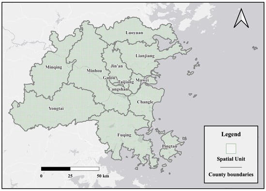
Figure 3.
Spatial distribution of the spatial units in the CrowdFZ dataset of Fuzhou.
Additionally, we collected the 2022 Point-of-Interest (POI) data and the 2023 road network data of Fuzhou to describe the geographical environments. The POI data were sourced from Gaode Map (https://lbs.amap.com/ (accessed on 11 May 2024)), while the road network data were obtained from OpenStreetMap (https://download.geofabrik.de (accessed on 21 November 2024)). The geographical environments include 22 external factors, denoted as . Specifically, we used the POI data to calculate the number of facilities in each spatial unit for the following categories: tourist attractions, transportation facilities, educational and cultural institutions, healthcare services, sports and fitness centers, leisure and entertainment venues, dining establishments, shopping locations, hotels and accommodations, life services, residential and commercial buildings, business enterprises, automotive services, and financial institutions, totaling 14 external factors. Using the road network data, we computed the distance from each spatial unit to primary roads, secondary roads, tertiary roads, and residential roads, as well as the length of these four types of roads within each spatial unit, totaling eight external factors.
5.2. Experiment Setting and Evaluation Metric
To ensure the fairness of the comparison, we adopted almost identical experimental settings for our proposed SCS-Net and the deep learning baselines. Specifically, we used the historical crowd flow data from the previous six time slices () to predict the next one or three time slices (). The last two weeks of the CrowdFZ dataset were used for testing, while 80% of the remaining data were randomly selected for training and 20% for validation. Min-max normalization was applied to scale the crowd flow and geographical environments into the range [0,1]. Moreover, the batch size was set to 16. The number of hidden states was set to 64. The convolution kernel size was set to 3. The random seed was set to 2025. We employed the Adam optimizer to optimize the model parameters with an initial learning rate of 0.001 and a maximum of 500 epochs. We applied the early stopping strategy to avoid overfitting, setting a patience of 10, which means training stopped if the validation loss did not improve for 10 consecutive epochs. The experiments were conducted using the PyTorch 1.13 framework on an NVIDIA Tesla V100 GPU server.
In particular, for the key hyperparameters of our proposed SCS-Net, we conducted a manual search over the following ranges: the number of clusters , the number of shared patterns , the weight for the clustering loss , and the weight for the compressive sensing loss . As shown in Figure 4, SCS-Net demonstrates relatively stable performance with small MAE and RMSE fluctuations across most parameter configurations. Based on the optimal parameter configuration, we selected , , , and as the default setting.
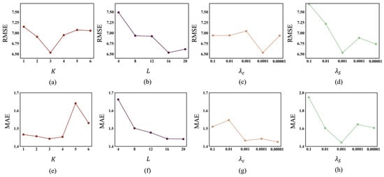
Figure 4.
Results of the parameter sensitivity analysis. (a–d) RMSE of SCS-Net under different hyperparameter configurations. (e–h) MAE of SCS-Net under different hyperparameter configurations.
In the experiments, we evaluated the models’ performance using two common metrics: Mean Absolute Error (MAE) and Root Mean Square Error (RMSE). They can be formulated as the following equations:
where denotes the L1 norm.
5.3. Model Accuracy
To evaluate the accuracy of our proposed SCS-Net for large-scale crowd flow prediction, we selected the following 11 baseline models for comparison. To ensure a fair comparison, we kept the hyperparameters of the baseline models as consistent as possible with those of the proposed SCS-Net. This includes settings such as batch size, number of hidden states, number of CNN layers, number of RNN layers, convolution kernel size, random seed, optimizer, learning rate and patience in early stopping strategy. Based on these aligned configurations, we then performed additional hyperparameter tuning for each baseline model to optimize their performance.
- HA: Historical Average is a classic non-parametric time series prediction method that uses the average of historical crowd flow as the predictions.
- GRU [46]: Gated Recurrent Unit is a classic deep learning time-series prediction model capable of capturing long-term temporal dependencies.
- DLinear [47]: DLinear is an advanced time series prediction model that decomposes historical data into trend and residual components, efficiently capturing long-term temporal dependencies through simple linear layers. The kernel size of the moving average operation was set to 5.
- ConvGRU [48]: Convolutional Gated Recurrent Unit is a classic CNN-based spatio-temporal prediction model that extends GRU with convolutional structures to capture spatio-temporal dependencies.
- STResNet [7]: Spatio-Temporal Residual Network is a widely recognized CNN-based crowd flow prediction model that employs residual units to capture spatio-temporal dependencies. The number of ResUnits was set to 3.
- AGCRN [49]: Adaptive Graph Convolutional Recurrent Network is a representative GNN-based spatio-temporal prediction model that extends GRU with adaptive graph convolution to capture spatio-temporal dependencies. The dimension of node embedding was set to 16.
- DeepCrowd [20]: DeepCrowd is the first model applied to large-scale crowd flow prediction. It constructs a pyramidal architecture by stacking ConvLSTM layers to capture large-scale spatial dependencies. The number of pyramidal ConvLSTM layers was set to 3.
- ASTCN [36]: Attentive Spatial–Temporal Convolutional Network is a representative attention-based crowd flow prediction model that introduces causal 3D convolutions and attention mechanisms to capture spatio-temporal dependencies. The number of ST blocks was set to 1.
- TLAE [50]: Temporal Latent Auto-Encoder is a representative prediction model incorporating compressive sensing, which achieves efficient predicting by compressing and reconstructing time series data. However, compared to SCS-Net, TLAE performs less comprehensive time-series modeling and overlooks residual learning. The latent dimension was set to 16.
- STRN [15]: Spatio-Temporal Relation Network is an advanced CNN-based crowd flow prediction model that introduces Mincut loss to extract the spatially stratified structure for modeling spatial heterogeneity. The number of regions was set to 3.
- BigST [51]: BigST is an advanced large-scale spatio-temporal prediction model that uses a pre-training strategy to extract long-term temporal representations and introduces a linearized global spatial convolution network to efficiently capture spatial dependencies. The size of time window in the long sequence feature extractor was set to 24. The dimension of random features was set to 32.
The accuracy comparison results of our proposed SCS-Net and the baseline models on the CrowdFZ dataset are shown in Table 1. Overall, SCS-Net significantly outperforms the baseline models across all metrics. Specifically, for the deep learning baseline models, the MAE increases by 35.5% to 120.3% and the RMSE increases by 26.3% to 74.7% in single-step predictions, while the MAE increases by 58.6% to 139.2% and the RMSE increases by 33.6% to 112.4% in multi-step predictions. This demonstrates the superior performance of SCS-Net in large-scale crowd flow prediction.

Table 1.
Accuracy comparison results of SCS-Net and baseline models on the CrowdFZ dataset. and represent the MAE and RMSE increase in the baseline models relative to SCS-Net, respectively. The underlined values indicate the best metrics among the baseline models. The bold values indicate the best metrics among all models.
Among the baseline models, the spatio-temporal prediction models outperform the time series prediction model, highlighting the importance of spatial dependency in large-scale crowd flow prediction. As the model architectures become more complex, the RMSE generally decreases. ASTCN and DeepCrowd, which have the most sophisticated structures, achieve the lowest RMSE among the baseline models. This is attributed to their incorporation of spatial downsampling techniques, which expand the spatial receptive field. These two models partially mitigate the impact of spatial heterogeneity, thereby enhancing performance. Although STRN models spatial heterogeneity, it enforces spatially compact and balanced clusters in the spatially stratified structure. This constraint misaligns with the urban functional layouts, ultimately limiting its accuracy.
However, the comparison results among the baseline models reveal an unusual phenomenon in the MAE metric. Specifically, the simpler models, ConvGRU and TLAE, achieve the lowest MAE among the baseline models, whereas the more complex ASTCN and DeepCrowd, which excel in RMSE, perform less satisfactorily in MAE. Unexpectedly, the GRU even achieves a lower MAE than ASTCN and DeepCrowd. To investigate this anomaly, we visualize the MAE distributions of single-step predictions for SCS-Net, TLAE, ASTCN, DeepCrowd, ConvGRU, and GRU (Figure 5). To enhance readability, we applied a natural logarithmic transformation, , to the MAE values. The results indicate that most MAEs are concentrated in the low-value range, as most spatial units exhibit relatively low human activity intensity in large-scale crowd flow prediction. Although ASTCN and DeepCrowd have larger medians and quartiles compared to the other models, their peak values are significantly lower. This suggests that ASTCN and DeepCrowd demonstrate a distinct advantage in predicting spatial units with higher human activity intensity (H-units) but struggle with those with lower human activity intensity (L-units). This may be attributed to the causal 3D convolutions in ASTCN and the pyramid ConvLSTMs in DeepCrowd, which enable both models to capture longer-range spatio-temporal dependencies and thus effectively fit the complex crowd flow patterns in H-units. However, H-units contribute more to the loss function. The two models tend to overfit in H-units and poorly generalize to the simpler patterns in L-units. Since most spatial units are L-units, the advantages of ASTCN and DeepCrowd are difficult to demonstrate in the first-order MAE metric, leading to better RMSE but worse MAE. In contrast, due to their simpler structures, TLAE, ConvGRU, and GRU prioritize the simpler crowd flow patterns in L-units, resulting in the underfitting of H-units. As second-order RMSE is more sensitive to peak values, these models achieve better MAE but worse RMSE.
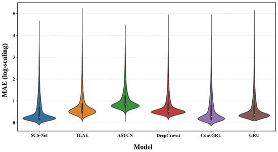
Figure 5.
MAE distributions of SCS-Net, TLAE, ASTCN, DeepCrowd, ConvGRU, and GRU after log-scaling. For each column, the outer curve illustrates the probability density distribution, the thick black bar in the center represents the interquartile range (IQR), the thin black lines extending from it denote the 95% confidence interval, and the white dot indicates the median.
Additionally, we visualized the prediction errors of an H-unit and an L-unit on 24 February 2023 (Figure 6). To maintain readability, we selected four representative models for comparison. H-unit A corresponds to Shangxiahang Historic District, a major tourist and commercial area in Fuzhou, while L-unit B corresponds to Gu’an Village, a small rural village in Fuzhou. The results show that ConvGRU and GRU exhibit larger error fluctuations in H-unit A, whereas their errors remain relatively stable in L-unit B. In contrast, ASTCN exhibits the opposite trend, further validating our understanding of this anomaly. Moreover, as shown in Figure 6, SCS-Net effectively captures the significant differences in crowd flow patterns between spatial units A and B, demonstrating its capability to handle spatial heterogeneity. As a result, it achieves the best overall performance.
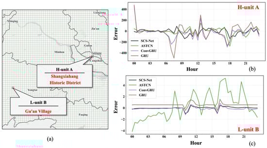
Figure 6.
Prediction errors of SCS-Net, ASTCN, ConvGRU, and GRU on H-unit A and L-unit B on 24 February 2023. (a) Locations of H-unit A and L-unit B. (b) Prediction errors for H-unit A. (c) Prediction errors for L-unit B.
5.4. Model Efficiency
To evaluate the efficiency of our proposed SCS-Net and the baseline models for large-scale crowd flow prediction, we introduced Giga Floating-Point Operations (GFLOPs) and training time (minutes) as evaluation metrics to assess model efficiency. The GFLOPs measures the total number of floating-point operations performed by the model per batch (batch size = 1). The training time reflects the actual time required for the models to converge during training. The efficiency comparison results are shown in Figure 7. Overall, the GFLOPs and the training time are correlated. SCS-Net significantly outperforms most baseline models. Although the GFLOPs and training time of HA and DLinear are considerably lower than that of SCS-Net, the poor predictive performance of these two linear time series prediction models limits their application to large-scale crowd flow prediction tasks. Meanwhile, TLAE also has lower GFLOPs and training time and achieves relatively good accuracy. However, when SCS-Net is deployable, it remains the better choice. In contrast, the CNN, GNN, and attention-based spatio-temporal prediction models have GFLOPs approximately 53 (ASTCN) to 1067 (DeepCrowd) times higher than SCS-Net and training times that are about 3.1 times (ASTCN) to 83.2 times (AGCRN) longer, leading to substantially higher costs. Considering that SCS-Net is not constrained by prior graph structures, nor by the shape or distribution of spatial units, this demonstrates its superior applicability to large-scale crowd flow prediction.
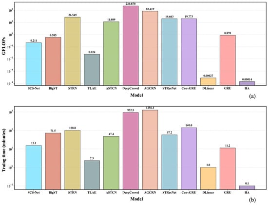
Figure 7.
Efficiency comparison results of SCS-Net and baseline models on the CrowdFZ dataset. (a) Comparison of GFLOPs. (b) Comparison of training time.
5.5. Ablation Experiment
To validate the effectiveness of the SS-Module and CS-Modules in our proposed SCS-Net, we designed three variants of SCS-Net and conduct ablation experiments on the CrowdFZ dataset.
- SCS-Net-g: Replaces the CS-Modules with a GRU, retaining the model’s predictive function while removing its capacity to perceive shared crowd flow patterns.
- SCS-Net-k: Replaces the SS-Module with K-means clustering based on geographical environments, providing a prior spatially stratified structure.
- SCS-Net-c: Removes the SS-Module entirely, making the model incapable of capturing the spatially stratified structure.
The comparison results of our proposed SCS-Net and its variants are shown in Table 2. Among the three variants, SCS-Net-g, which removes the compressive sensing component, experiences the most significant performance degradation. This highlights the critical contribution of the CS-Modules to the superior performance of SCS-Net. Specifically, the CS-Modules learn shared crowd flow patterns, preventing SCS-Net from being disturbed by redundant information among spatial units, thereby enhancing its sensitivity to individual spatial unit differences. Moreover, the results of SCS-Net-k and SCS-Net-c are close, indicating that prior K-means clustering fails to effectively capture the spatially stratified structure suitable for large-scale crowd flow prediction. In contrast, the SS-Module adaptively learns this structure in a posterior manner during the prediction process, further enhancing the model’s predictive performance.
Table 2.
Comparison results of SCS-Net and its variants on the CrowdFZ dataset. and represent the MAE and RMSE increase in the variants relative to SCS-Net, respectively. The bold values indicate the best metrics among all models.
5.6. Analysis of the Spatially Stratified Structure
The spatially stratified structure not only improves the accuracy of crowd flow prediction but also offers deeper insights into spatial heterogeneity of human mobility. To explore this, we visualized the spatial distributions of clusters produced by the prior K-means and the posterior SS-Module, and Fuzhou’s actual road network, as shown in Figure 8. Overall, both clustering methods produce clusters with similar meanings: Cluster 1 (C-1) represents H-units with high crowd activity, while Cluster 0 (C-0) and Cluster 2 (C-2) correspond to L-units with low and even lower activity, respectively. The distribution of C-0 is relatively consistent between the two methods, but C-1 and C-2 show notable differences. Compared to Fuzhou’s road network, the C-1 from K-means aligns with the core urban area, whereas the C-1 from the SS-Module matches the built-up areas, reflecting the city’s urban development boundary. Since the ablation experiments show that the SS-Module’s clustering better captures the spatially stratified structure for crowd flow prediction in Fuzhou, this suggests that effectively handling large-scale, city-level tasks requires the ability to distinguish and model the crowd flow patterns in built-up and non-built-up areas.
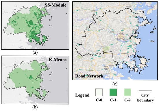
Figure 8.
Comparison of clustering results between K-means and the SS-Module. (a) Spatial distribution of clusters produced by K-means. (b) Spatial distribution of clusters produced by the SS-Module. (c) Actual road network of Fuzhou. In the legend, “C-0”, “C-1”, and “C-2” represent Cluster 0, Cluster 1, and Cluster 2 in both clustering results, respectively.
To further investigate which external factors play a key role in identifying the spatially stratified structure, we built regression models using the random forest algorithm to relate the external factors to each cluster from the SS-Module. We then visualized the distribution of normalized feature importances for these clusters, as shown in Figure 9. Overall, road network-related factors dominate the feature importance across all three clusters. Specifically, distance to primary roads, distance to residential roads, and residential road length are critical for identifying C-0 and C-2, likely reflecting proximity to built-up areas. In contrast, identifying C-1, which represents built-up areas, requires considering more factors, including residential road length, distance to residential roads, distance to primary roads, life services, shopping locations, educational and cultural institutions, and tourist attractions. These factors are closely related to transport accessibility and diverse urban functions, offering potential value for urban spatial planning in Fuzhou. The prior K-means clustering fails to capture the complex relationships between crowd flow and these factors, thereby limiting its ability to improve prediction performance.
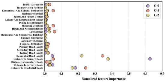
Figure 9.
Random forest normalized feature importances for each cluster in the SS-Module.
6. Conclusions
In this paper, we propose SCS-Net for accurate and efficient large-scale crowd flow prediction. In the model, we develop a Spatially Stratified Module (SS-Module) that adaptively extracts the underlying spatially stratified structure in a posterior manner, thereby improving prediction accuracy. Based on this, several Compressive Sensing Modules (CS-Modules) are developed to compress redundant information in crowd flow and learn shared crowd flow patterns, enhancing model efficiency. We conduct extensive experiments on a large-scale real-world crowd flow prediction dataset. The results show that SCS-Net achieves superior accuracy, outperforming deep learning baseline models by 35.25–139.2% in MAE and 26.3–112.4% in RMSE. In terms of efficiency, the GFLOPs and the training time of the prevalent spatio-temporal prediction models are approximately 53 to 1067 times and 3.1 to 83.2 times higher than SCS-Net, respectively. Additionally, ablation experiments on several variants of SCS-Net validate the effectiveness of the SS-Module and CS-Modules. Further analysis of the spatially stratified structure reveals that spatial heterogeneity in crowd flow patterns is closely related to the urban road network.
However, there are several limitations in this study. First, the generalizability and applicability of our proposed SCS-Net need to be further validated through experiments in additional study areas. Second, since quantifying predictive uncertainty is also crucial for the applications of crowd flow prediction, we plan to incorporate techniques such as Monte-Carlo dropout, quantile regression, and deep ensembles in the future work to enhance the model’s robustness and interpretability. Moreover, for long-term and large-scale crowd flow prediction tasks, we will explore more efficient and effective solutions, as modeling more temporal slices may reduce model efficiency and lead to vanishing gradient issues. Meanwhile, future crowd flow is influenced not only by historical trends but also by data incompleteness (e.g., sparsity and missing values) and anomalous events (e.g., concerts and public holidays). Capturing the impact of these external disruptions is another challenge we aim to address. This will further support urban management and public safety.
Author Contributions
Conceptualization, X.T. and K.C.; methodology, X.T.; software, X.T.; validation X.T. and K.C.; formal analysis X.T.; data curation X.T., B.L., Z.Z., Y.T. and S.W.; writing—original draft preparation, X.T.; writing—review and editing, X.T., K.C. and M.D.; visualization, X.T.; supervision, K.C., M.D. and B.L.; funding acquisition, K.C., M.D. and B.L. All authors have read and agreed to the published version of the manuscript.
Funding
This research was funded by the National Natural Science Foundation of China (grant number 42430110 and 42171459) and the Natural Science Foundation of Hunan Province (grant number 2024JJ1009).
Data Availability Statement
The datasets presented in this article are not readily available due to privacy restrictions and cooperation agreements with Chinese telecom operators. Requests for access to the datasets should be directed to the corresponding author. We confirm that all figures and tables in this article were originally created by the authors with data or results from this study. There are no copyright issues associated with these figures and tables, and no permissions are required for their use or reference.
Acknowledgments
This work was carried out in part using computing resources at the High-Performance Computing Platform of Central South University.
Conflicts of Interest
The authors declare that they have no conflicts of interest.
References
- Sun, L.; Chen, J.; Li, Q.; Huang, D. Dramatic Uneven Urbanization of Large Cities throughout the World in Recent Decades. Nat. Commun. 2020, 11, 5366. [Google Scholar] [CrossRef]
- Mahtta, R.; Fragkias, M.; Güneralp, B.; Mahendra, A.; Reba, M.; Wentz, E.A.; Seto, K.C. Urban Land Expansion: The Role of Population and Economic Growth for 300+ Cities. npj Urban Sustain. 2022, 2, 5. [Google Scholar] [CrossRef]
- Zheng, Y.; Capra, L.; Wolfson, O.; Yang, H. Urban Computing: Concepts, Methodologies, and Applications. ACM Trans. Intell. Syst. Technol. 2014, 5, 1–55. [Google Scholar] [CrossRef]
- Chen, K.; Chu, G.; Yang, X.; Shi, Y.; Lei, K.; Deng, M. HSETA: A Heterogeneous and Sparse Data Learning Hybrid Framework for Estimating Time of Arrival. IEEE Trans. Intell. Transp. Syst. 2022, 23, 21873–21884. [Google Scholar] [CrossRef]
- Wang, P.; Zhang, Y.; Hu, T.; Zhang, T. Urban Traffic Flow Prediction: A Dynamic Temporal Graph Network Considering Missing Values. Int. J. Geogr. Inf. Sci. 2023, 37, 885–912. [Google Scholar] [CrossRef]
- Hoang, M.X.; Zheng, Y.; Singh, A.K. FCCF: Forecasting Citywide Crowd Flows Based on Big Data. In Proceedings of the 24th ACM SIGSPATIAL International Conference on Advances in Geographic Information Systems, Burlingame, CA, USA, 31 October–3 November 2016; pp. 1–10. [Google Scholar]
- Zhang, J.; Zheng, Y.; Qi, D. Deep Spatio-Temporal Residual Networks for Citywide Crowd Flows Prediction. In Proceedings of the AAAI Conference on Artificial Intelligence, San Francisco, CA, USA, 4–9 February 2017; Volume 31. [Google Scholar] [CrossRef]
- Dai, G.; Huang, H.; Peng, X.; Zhang, B.; Fu, X. ARFGCN: Adaptive Receptive Field Graph Convolutional Network for Urban Crowd Flow Prediction. Mathematics 2024, 12, 1739. [Google Scholar] [CrossRef]
- Zhang, J.; Zheng, Y.; Qi, D.; Li, R.; Yi, X.; Li, T. Predicting Citywide Crowd Flows Using Deep Spatio-Temporal Residual Networks. Artif. Intell. 2018, 259, 147–166. [Google Scholar] [CrossRef]
- Xie, P.; Li, T.; Liu, J.; Du, S.; Yang, X.; Zhang, J. Urban Flow Prediction from Spatiotemporal Data Using Machine Learning: A Survey. Inf. Fusion 2020, 59, 1–12. [Google Scholar] [CrossRef]
- Wang, P.; Zhang, T.; Zhang, H.; Cheng, S.; Wang, W. Adding Attention to the Neural Ordinary Differential Equation for Spatio-Temporal Prediction. Int. J. Geogr. Inf. Sci. 2024, 38, 156–181. [Google Scholar] [CrossRef]
- Chen, K.; Deng, M.; Lei, K.; Liu, Q.; Shi, Y. Adaptive Multi-View Neural Network for Network-Wide and Segment-Wise Traffic Speed Estimation With Heterogeneous Missing Cases. Trans. GIS 2025, 29, e13295. [Google Scholar] [CrossRef]
- Xu, L.; Chen, N.; Chen, Z.; Zhang, C.; Yu, H. Spatiotemporal Forecasting in Earth System Science: Methods, Uncertainties, Predictability and Future Directions. Earth-Sci. Rev. 2021, 222, 103828. [Google Scholar] [CrossRef]
- Luo, P.; Song, Y.; Zhu, D.; Cheng, J.; Meng, L. A Generalized Heterogeneity Model for Spatial Interpolation. Int. J. Geogr. Inf. Sci. 2023, 37, 634–659. [Google Scholar] [CrossRef]
- Liang, Y.; Ouyang, K.; Sun, J.; Wang, Y.; Zhang, J.; Zheng, Y.; Rosenblum, D.; Zimmermann, R. Fine-Grained Urban Flow Prediction. In Proceedings of the Web Conference 2021, Ljubljana, Slovenia, 19–23 April 2021; pp. 1833–1845. [Google Scholar]
- Huang, W.; Li, S.; Liu, X.; Ban, Y. Predicting Human Mobility with Activity Changes. Int. J. Geogr. Inf. Sci. 2015, 29, 1569–1587. [Google Scholar] [CrossRef]
- Zhang, Y.; Wu, S.; Zhao, Z.; Yang, X.; Fang, Z. An Urban Crowd Flow Model Integrating Geographic Characteristics. Sci. Rep. 2023, 13, 1695. [Google Scholar] [CrossRef] [PubMed]
- Lei, K.; Chen, K.; Deng, M.; Tan, X.; Yang, W.; Liu, H.; Huang, C. CSSKL: Collaborative Specific-Shared Knowledge Learning Framework for Cross-City Spatiotemporal Forecasting in Cellular Networks. Int. J. Geogr. Inf. Sci. 2025, 1–38. [Google Scholar] [CrossRef]
- Lin, Y.; Huang, J.; Sun, D. A Novel Recurrent Convolutional Network Based on Grid Correlation Modeling for Crowd Flow Prediction. J. King Saud Univ.-Comput. Inf. Sci. 2023, 35, 101699. [Google Scholar] [CrossRef]
- Jiang, R.; Cai, Z.; Wang, Z.; Yang, C.; Fan, Z.; Chen, Q.; Tsubouchi, K.; Song, X.; Shibasaki, R. DeepCrowd: A Deep Model for Large-Scale Citywide Crowd Density and Flow Prediction. IEEE Trans. Knowl. Data Eng. 2021, 35, 276–290. [Google Scholar] [CrossRef]
- Zhang, X.; Sun, Y.; Guan, F.; Chen, K.; Witlox, F.; Huang, H. Forecasting the Crowd: An Effective and Efficient Neural Network for Citywide Crowd Information Prediction at a Fine Spatio-Temporal Scale. Transp. Res. Part C Emerg. Technol. 2022, 143, 103854. [Google Scholar] [CrossRef]
- Wang, P.; Zhang, H.; Liu, J.; Lu, F.; Zhang, T. Efficient Inference of Large-Scale Air Quality Using a Lightweight Ensemble Predictor. Int. J. Geogr. Inf. Sci. 2025, 39, 900–924. [Google Scholar] [CrossRef]
- Medina-Salgado, B.; Sánchez-DelaCruz, E.; Pozos-Parra, P.; Sierra, J.E. Urban Traffic Flow Prediction Techniques: A Review. Sustain. Comput. Inform. Syst. 2022, 35, 100739. [Google Scholar] [CrossRef]
- Zhang, J.; Zheng, Y.; Qi, D.; Li, R.; Yi, X. DNN-Based Prediction Model for Spatio-Temporal Data. In Proceedings of the 24th ACM SIGSPATIAL International Conference on Advances in Geographic Information Systems, Burlingame, CA, USA, 31 October–3 November 2016; pp. 1–4. [Google Scholar]
- Zheng, C.; Fan, X.; Wen, C.; Chen, L.; Wang, C.; Li, J. DeepSTD: Mining Spatio-Temporal Disturbances of Multiple Context Factors for Citywide Traffic Flow Prediction. IEEE Trans. Intell. Transp. Syst. 2020, 21, 3744–3755. [Google Scholar] [CrossRef]
- Lin, Z.; Feng, J.; Lu, Z.; Li, Y.; Jin, D. DeepSTN+: Context-Aware Spatial-Temporal Neural Network for Crowd Flow Prediction in Metropolis. In Proceedings of the AAAI Conference on Artificial Intelligence, Honolulu, HI, USA, 27 January–1 February 2019; Volume 33, pp. 1020–1027. [Google Scholar] [CrossRef]
- Go, H.; Park, S. A Study on Deep Learning Model Based on Global–Local Structure for Crowd Flow Prediction. Sci. Rep. 2024, 14, 12623. [Google Scholar] [CrossRef]
- Jin, W.; Lin, Y.; Wu, Z.; Wan, H. Spatio-Temporal Recurrent Convolutional Networks for Citywide Short-Term Crowd Flows Prediction. In Proceedings of the 2nd International Conference on Compute and Data Analysis, DeKalb, IL, USA, 23–25 March 2018; pp. 28–35. [Google Scholar]
- Yuan, X.; Han, J.; Wang, X.; He, Y.; Xu, W.; Zhang, K. A Novel Learning Approach for Citywide Crowd Flow Prediction. In Proceedings of the 2019 Computing, Communications and IoT Applications (ComComAp), Shenzhen, China, 26–28 October 2019; pp. 341–346. [Google Scholar]
- Ren, Y.; Chen, H.; Han, Y.; Cheng, T.; Zhang, Y.; Chen, G. A Hybrid Integrated Deep Learning Model for the Prediction of Citywide Spatio-Temporal Flow Volumes. Int. J. Geogr. Inf. Sci. 2020, 34, 802–823. [Google Scholar] [CrossRef]
- Tang, G.; Li, B.; Dai, H.-N.; Zheng, X. SPRNN: A Spatial–Temporal Recurrent Neural Network for Crowd Flow Prediction. Inf. Sci. 2022, 614, 19–34. [Google Scholar] [CrossRef]
- Wang, X.; Zhou, Z.; Zhao, Y.; Zhang, X.; Xing, K.; Xiao, F.; Yang, Z.; Liu, Y. Improving Urban Crowd Flow Prediction on Flexible Region Partition. IEEE Trans. Mob. Comput. 2020, 19, 2804–2817. [Google Scholar] [CrossRef]
- Cardia, M.; Luca, M.; Pappalardo, L. Enhancing Crowd Flow Prediction in Various Spatial and Temporal Granularities. In Proceedings of the Companion Proceedings of the Web Conference 2022, Virtual Event, Lyon, France, 25–29 April 2022; pp. 1251–1259. [Google Scholar]
- Ul Abideen, Z.; Sun, X.; Sun, C. Crowd Flow Prediction: An Integrated Approach Using Dynamic Spatial–Temporal Adaptive Modeling for Pattern Flow Relationships. J. Forecast. 2025, 44, 556–574. [Google Scholar] [CrossRef]
- Li, F.; Feng, J.; Yan, H.; Jin, D.; Li, Y. Crowd Flow Prediction for Irregular Regions with Semantic Graph Attention Network. ACM Trans. Intell. Syst. Technol. 2022, 13, 1–14. [Google Scholar] [CrossRef]
- Guo, H.; Zhang, D.; Jiang, L.; Poon, K.-W.; Lu, K. ASTCN: An Attentive Spatial–Temporal Convolutional Network for Flow Prediction. IEEE Internet Things J. 2022, 9, 3215–3225. [Google Scholar] [CrossRef]
- Ali, A.; Zhu, Y.; Zakarya, M. Exploiting Dynamic Spatio-Temporal Correlations for Citywide Traffic Flow Prediction Using Attention Based Neural Networks. Inf. Sci. 2021, 577, 852–870. [Google Scholar] [CrossRef]
- Xie, Y.; Niu, J.; Zhang, Y.; Ren, F. Multisize Patched Spatial-Temporal Transformer Network for Short- and Long-Term Crowd Flow Prediction. IEEE Trans. Intell. Transp. Syst. 2022, 23, 21548–21568. [Google Scholar] [CrossRef]
- Zheng, Z.; Gu, J.; Zhou, Q.; Lu, X. Prediction in Long-Term Evolution: Exploiting the Interaction between Urban Crowd Flow Variation and POI Transition Patterns. In Proceedings of the 2023 IEEE International Conference on Data Mining (ICDM), Shanghai, China, 1–4 December 2023; pp. 1559–1564. [Google Scholar]
- Jiang, R.; Cai, Z.; Wang, Z.; Yang, C.; Fan, Z.; Chen, Q.; Song, X.; Shibasaki, R. Predicting Citywide Crowd Dynamics at Big Events: A Deep Learning System. ACM Trans. Intell. Syst. Technol. 2022, 13, 1–24. [Google Scholar] [CrossRef]
- Yuan, Y.; Ding, J.; Feng, J.; Jin, D.; Li, Y. UniST: A Prompt-Empowered Universal Model for Urban Spatio-Temporal Prediction. In Proceedings of the Proceedings of the 30th ACM SIGKDD Conference on Knowledge Discovery and Data Mining, Barcelona, Spain, 25–29 August 2024; pp. 4095–4106. [Google Scholar]
- Su, C.; Wu, C.; Lian, D. GridFormer: Spatial-Temporal Transformer Network for Citywide Crowd Flow Prediction. In Frontiers in Artificial Intelligence and Applications; Gal, K., Nowé, A., Nalepa, G.J., Fairstein, R., Rădulescu, R., Eds.; IOS Press: Amsterdam, The Netherlands, 2023; ISBN 978-1-64368-436-9. [Google Scholar]
- Zhu, A.; Lu, G.; Liu, J.; Qin, C.; Zhou, C. Spatial Prediction Based on Third Law of Geography. Ann. GIS 2018, 24, 225–240. [Google Scholar] [CrossRef]
- Deng, M.; Yang, W.; Liu, Q.; Jin, R.; Xu, F.; Zhang, Y. Heterogeneous Space–Time Artificial Neural Networks for Space–Time Series Prediction. Trans. GIS 2018, 22, 183–201. [Google Scholar] [CrossRef]
- Zhang, C.; Zhang, H.; Qiao, J.; Yuan, D.; Zhang, M. Deep Transfer Learning for Intelligent Cellular Traffic Prediction Based on Cross-Domain Big Data. IEEE J. Sel. Areas Commun. 2019, 37, 1389–1401. [Google Scholar] [CrossRef]
- Chung, J.; Gulcehre, C.; Cho, K.; Bengio, Y. Empirical Evaluation of Gated Recurrent Neural Networks on Sequence Modeling. arXiv 2014, arXiv:1412.3555. [Google Scholar]
- Zeng, A.; Chen, M.; Zhang, L.; Xu, Q. Are Transformers Effective for Time Series Forecasting? In Proceedings of the AAAI Conference on Artificial Intelligence, Washington, DC, USA, 7–14 February 2023; Volume 37, pp. 11121–11128. [Google Scholar] [CrossRef]
- Ballas, N.; Yao, L.; Pal, C.; Courville, A. Delving Deeper into Convolutional Networks for Learning Video Representations. arXiv 2015, arXiv:1511.06432. [Google Scholar]
- Bai, L.; Yao, L.; Li, C.; Wang, X.; Wang, C. Adaptive Graph Convolutional Recurrent Network for Traffic Forecasting. Adv. Neural Inf. Process. Syst. 2020, 33, 17804–17815. [Google Scholar]
- Nguyen, N.; Quanz, B. Temporal Latent Auto-Encoder: A Method for Probabilistic Multivariate Time Series Forecasting. In Proceedings of the AAAI Conference on Artificial Intelligence, Virtual Event, 2–9 February 2021; Volume 35, pp. 9117–9125. [Google Scholar] [CrossRef]
- Han, J.; Zhang, W.; Liu, H.; Tao, T.; Tan, N.; Xiong, H. BigST: Linear Complexity Spatio-Temporal Graph Neural Network for Traffic Forecasting on Large-Scale Road Networks. Proc. VLDB Endow. 2024, 17, 1081–1090. [Google Scholar] [CrossRef]
Disclaimer/Publisher’s Note: The statements, opinions and data contained in all publications are solely those of the individual author(s) and contributor(s) and not of MDPI and/or the editor(s). MDPI and/or the editor(s) disclaim responsibility for any injury to people or property resulting from any ideas, methods, instructions or products referred to in the content. |
© 2025 by the authors. Licensee MDPI, Basel, Switzerland. This article is an open access article distributed under the terms and conditions of the Creative Commons Attribution (CC BY) license (https://creativecommons.org/licenses/by/4.0/).