Hybrid Chebyshev-Type Methods for Solving Nonlinear Equations

Abstract

Chebyshev-type methods have replaced the Chebyshev method in practice for solving nonlinear equations in abstract spaces. These methods are of the same R-order of three. However, they are easier to deal with, since the computationally expensive second derivative of the operator involved does not appear on these methods. However, the invertibility of the first derivative is still required at each step of the iteration. In this article, the inverse is replaced by a finite sum of linear operators. The convergence of the new Hybrid Chebyshev-Type Method (HCTM) is established under relaxed generalized continuity assumptions on the derivative and majorizing sequences. The iterates of the new methods converge to the original ones, but they are easier to find. Moreover, the numerical examples demonstrate that the new iterates converge essentially as fast to the solution. The methodology of this article can be used on other methods with inverses along the same lines due to its generality.

1. Introduction

Let $X,Y$ denote Banach spaces and $D\subset X$ be a convex open set. A plethora of problems can be written using mathematical modeling like the following:

$$\begin{array}{c}\hfill \Lambda (x)=0,\end{array}$$

(1)

where $\Lambda :D\subset X⟶Y$ is a Fréchet-differentiable operator [1,2,3,4,5,6,7,8]. A solution $x^{*}\in D$ is needed in closed form. However, this is achievable only in special cases. That is why mostly iterative methods have been used to produce sequences converging to $x^{*}.$

Newton’s is without a doubt the most popular among methods of convergence of order two. It is defined for $x_0\in D$ and all $n=0,1,2,\dots$ by the following:

$$\begin{array}{c}\hfill x_{n+1}=x_n-{\Lambda }^{\prime }{(x_n)}^{-1}\Lambda (x_n).\end{array}$$

(2)

The implementation of Newton’s method requires the inversion of the linear operator ${\Lambda }^{\prime }(x_n)$ at each step, which may not be possible or computationally expensive. That is why in [9], we suggested hybrid Newton and Newton-like methods. In the case of Newton’s method, the hybrid analog is defined for $M\in \mathcal{L}(X,Y)$ (the space of all linear operators that are bounded) being an invertible operator, $\Delta =M^{-1}(M-{\Lambda }^{\prime }(x))$ and $B=B_m(x)=I+\Delta +\dots +{\Delta }^k,k$ being a natural number by the following:

$$\begin{array}{c}\hfill x_{n+1}=x_n-B{M}^{-1}\Lambda (x_n).\end{array}$$

(3)

Note, that ${lim}_{k⟶+\infty }{B}_m{M}^{-1}={\Lambda }^{\prime }.$ The inverse of the linear operator is computed only once. The convergence analysis of method (3) and the numerical examples demonstrate that the number of iterations needed to reach the same error tolerance for (2) and (3) is essentially the same. Motivated by these developments and in order to consider methods of an order higher than two, we look at the Chebyshev method [10,11,12,13]:

$$\begin{array}{c}\hfill x_{n+1}=x_n-{\Lambda }^{\prime }{(x_n)}^{-1}\Lambda (x_n)-{\displaystyle \frac{1}{2}}{\Lambda }^{\prime }{(x_n)}^{-1}{\Lambda }^{″}(x_n){\Lambda }^{\prime }{(x_n)}^{-1}\Lambda (x_n),\end{array}$$

(4)

and an optimization of the Chebysehev method:

$$\begin{array}{ccc}\hfill y_n& =& x_n-{\Lambda }^{\prime }{(x_n)}^{-1}\Lambda (x_n),\hfill \\ \hfill z_n& =& x_n+\lambda (y_n-x_n),\lambda \in (0,1],\hfill \\ \hfill A_n& =& A(x_n,z_n)={\displaystyle \frac{1}{\lambda }}{\Lambda }^{\prime }{(x_n)}^{-1}({\Lambda }^{\prime }(x_n)-{\Lambda }^{\prime }(z_n)),\hfill \\ \hfill x_{n+1}& =& y_n+{\displaystyle \frac{1}{2}}{A}_n(y_n-x_n).\hfill \end{array}$$

(5)

Method (5) is of R-order three but does not require the computation of ${\Lambda }^{″}(x_n)$ at each step as in (4), which is also of order three [10,11,12,13]. However, the implementation of (5) presents the same difficulties as (2). That is why we introduce the HCTM defined by the following:

$$\begin{array}{ccc}\hfill y_n& =& x_n-B{M}^{-1}\Lambda (x_n),\hfill \\ \hfill z_n& =& x_n+\lambda (y_n-x_n),\lambda \in (0,1],\hfill \\ \hfill A^1(x_n,z_n)& =& {\displaystyle \frac{1}{\lambda }}B{M}^{-1}({\Lambda }^{\prime }(x_n)-{\Lambda }^{\prime }(z_n)),\hfill \\ \hfill x_{n+1}& =& y_n+{\displaystyle \frac{1}{2}}{A}^1(x_n,z_n)(y_n-x_n).\hfill \end{array}$$

(6)

In this article, we study the local as well as the semi-local analysis of methods (5) and (6). The analysis of convergence relies on generalized continuity assumptions, which relax the usual Lipschitz or Hölder conditions on ${\Lambda }^{\prime }.$ In particular, the semi-local analysis also uses majorizing sequences to control the sequence $\left\{x_n\right\}.$ The conclusions are the same as the case of methods (2) and (3).

The following definitions are used in this paper.

Definition 1.

The computational order of convergence of a sequence ${\left\{x_n\right\}}_{n\ge 0}$ is defined by the following:

$${\overline{\rho }}_n={\displaystyle \frac{ln|e_{n+1}/e_n|}{ln|e_n/e_{n-1}|}},$$

where $x_{n-1},x_n,x_{n+1}$ are three consecutive iterations near the root α and $e_n=x_n-\alpha$ [7,12,14].

Definition 2.

The approximated computational order of convergence of a sequence ${\left\{x_n\right\}}_{n\ge 0}$ is defined by the following:

$${\widehat{\rho }}_n={\displaystyle \frac{ln|{\widehat{e}}_{n+1}/{\widehat{e}}_n|}{ln|{\widehat{e}}_n/{\widehat{e}}_{n-1}|}},$$

where ${\widehat{e}}_n=x_n-x_{n-1}.$$x_n,x_{n-1},x_{n-2}$ are three consecutive iterates [7,12,14].

The rest of the article is structured as follows. The local followed by semi-local analyses of method (5) are presented in Section 2 and Section 3, respectively. The same is carried out for method (6) in Section 4 and Section 5. The numerical examples can be found in Section 6 and the conclusions in Section 7.

2. Local Analysis of Method (5)

The analysis uses certain criteria. Let $T=[0,+\infty ).$ It is also convenient to employ the abbreviations CNDF for a continuous and nondecreasing function and SPS for the smallest positive solution. Suppose the following:

(H1)

There exists a CNDF $w_0:T⟶T$ such that the equation $w_0(t)-1=0$ has an SPS. Denote such a solution by ${\rho }_0.$ Set $T_0=[0,{\rho }_0).$

(H2)

There exists a CNDF $w:T_0⟶T$ for function $h_1:T_0⟶T$ defined by the following:

$$h_1(t)={\displaystyle \frac{{\int }_0^{1}w((1-\theta )t)d\theta }{1-w_0(t)}}$$

such that the equation $h_1(t)-1=0$ has an SPS in the interval $(0,{\rho }_0).$ Denote such a solution by $r_1.$

(H3)

For the function $h_2:T_0⟶T$ defined by $h_2(t)=[(1-\lambda )+\lambda h_1(t)]t,$ the equation $h_2(t)-1=0$ has an SPS in $(0,{\rho }_0$). Denote such a solution by $r_2.$

Denote the functions $\overline{w}:T_0⟶T,\tilde{w}:T_0⟶T$ and $h_3:T_0⟶T$ by the following:

$$\overline{w}(t)=\left\{\begin{array}{c}w((1+h_2(t))t\\ or\\ w_0(t)+w_0(h_2(t)t),\end{array}\right.$$

$$\tilde{w}(t)={\displaystyle \frac{1}{2\lambda }}{\displaystyle \frac{\overline{w}(t)}{1-w_0(t)}}$$

and

$$h_3(t)=(\tilde{w}(t)+(1+\tilde{w}(t))h_1(t))t.$$

Note, that in practice, we select the smallest of the two versions of the functions $\overline{w}$ and $\tilde{w}.$ The real functions $h_1,h_2$ and $h_3$ are used to majorize the error distances appearing in Theorem 1 that follows.

(H4)

The equation $h_3(t)-1=0$ has an SPS in $(0,{\rho }_0).$ Denote such a solution by $r_3.$ Set

$$r=min\left\{r_j\right\},j=1,2,3$$

(7)

and $T-1=[0,r].$ It follows by these definitions that for all $t\in T_1$,

$$0\le w_0(t)<1$$

(8)

and

$$0\le h_j(t)<1.$$

(9)

There exists a relationship between the functions $w_0$ and w with the operators on method (5).

(H5)

There exists a solution $x^{*}\in D$ of the equation $\Lambda (x)=0$ and an invertible operator $M\in L(X,Y)$ such that for each $u\in D$

$$\parallel M^{-1}({\Lambda }^{\prime }(u)-M)\parallel \le w_0(\parallel u-x^{*}\parallel ).$$

Set $D_0=D\cap S(x^{*},{\rho }_0).$ The notation $S(x^{*},{\rho }_0)$ denotes the open ball with a center at $x^{*}$ and a radius ${\rho }_0.$ Moreover, $S[x^{*},{\rho }_0)]$ is its closure.

(H6)

$\parallel M^{-1}({\Lambda }^{\prime }(u_2)-{\Lambda }^{\prime }(u_1))\parallel \le w(\parallel u_2-u_1\parallel )$ for each $u_1,u_2\in D_0$

and

(H7)

$S[x^{*},r]\subset D.$

Remark 1.

(i)

The parameter r is shown to be a radius of convergence for the sequence $\left\{x_n\right\}$ given by formula (5) in Theorem 1.

(ii)

Some choices for M can be $M=I,$ where I is the identity operator on X or $M={\Lambda }^{\prime }(x^{*}).$ In the latter case, $x^{*}$ is a simple solution. Note, that this is not assumed or necessarily implied by conditions (H1)–(H2). Consequently, method (5) can be used to find solutions $x^{*}$ of a multiplicity greater than one. Other choices for M are also possible, provided that criteria (H5) and (H6) hold such that $M={\Lambda }^{\prime }(\overline{x}),$ where $\overline{x}\in D$ is an auxiliary point [11].

(iii)

The smaller of the two versions of the function $\overline{w}$ is used. However, if these versions cross on the interval $T_0,$ say, e.g., as

$$w((1+h_2(t))t)\le w_0(t)+w_0(h_2(t)t)$$

for $t\in [0,{\overline{\rho }}_0]$ and

$$w_0(t)+w_0(h_2(t)t)\le w((1+h_2(t))t)$$

for $t\in [{\overline{\rho }}_0,{\rho }_0],$ where ${\overline{\rho }}_0\in [0,{\rho }_0],$ then we choose

$$\overline{w}(t)=\left\{\begin{array}{cc}w((1+h_2(t))t)& fort\in [0,{\overline{\rho }}_0]\\ w_0(t)+w_0(h_2(t)t)& fort\in [{\overline{\rho }}_0,{\rho }_0].\end{array}\right.$$

The local analysis of convergence uses conditions (H1)–(H7) and the preceding notation. Let $D_1=S(x^{*},r)-\left\{x^{*}\right\}.$

Theorem 1.

Suppose that criteria (H1)–(H7) hold and $x_0\in D_1.$ Then, the following assertions hold for method (5) and all $n=0,1,2,\dots$:

$$\left\{x_n\right\}\subset S(x^{*},r),$$

(10)

$$\parallel y_n-x^{*}\parallel \le h_1(\parallel x_n-x^{*}\parallel )\parallel x_n-x^{*}\parallel \le \parallel x_n-x^{*}\parallel <r,$$

(11)

$$\parallel z_n-x^{*}\parallel \le h_2(\parallel x_n-x^{*}\parallel )\parallel x_n-x^{*}\parallel \le \parallel x_n-x^{*}\parallel ,$$

(12)

$$\parallel x_{n+1}-x^{*}\parallel \le h_3(\parallel x_n-x^{*}\parallel )\parallel x_n-x^{*}\parallel \le \parallel x_n-x^{*}\parallel$$

(13)

and the sequence $\left\{x_n\right\}$ converges to $x^{*}.$

Proof. 

Induction on n shall establish assertions (10)–(12). Clearly, Equation (10) holds if $n=0.$ Let $u\in S(x^{*},r).$ It follows by (7), (8), and (H5) that:

$$\parallel M^{-1}({\Lambda }^{\prime }(u)-M)\parallel \le w_0(\parallel u-x^{*}\parallel )\le w_0(r)<1.$$

(14)

The estimate (14) and the Banach standard perturbation Lemma on linear operators [10,13,15,16,17] imply that ${\Lambda }^{\prime }{(u)}^{-1}\in L(Y,X)$ and

$$\parallel {\Lambda }^{\prime }{(u)}^{-1}M\parallel \le {\displaystyle \frac{1}{1-w_0(\parallel u-x^{*}\parallel )}}.$$

(15)

In particular, if $u=x_0,$ then ${\Lambda }^{\prime }{(x_0)}^{-1}\in L(Y,X),$ the iterate $y_0$ is well-defined, and we can write as follows:

$$\begin{array}{ccc}\hfill y_0-x^{*}& =& x_0-x^{*}-{\Lambda }^{\prime }{(x_0)}^{-1}\Lambda (x_0)\hfill \\ \hfill & =& [{\Lambda }^{\prime }{(x_0)}^{-1}{\Lambda }^{\prime }(x^{*})]{\int }_0^1{\Lambda }^{\prime }{(x^{*})}^{-1}[{\Lambda }^{\prime }(x^{*}+\theta (x_0-x^{*}))\hfill \\ \hfill & & -{\Lambda }^{\prime }(x_0)]d\theta (x_0-x^{*}).\hfill \end{array}$$

(16)

By applying (7), (9) (for $j=1$), Equation (15) (for $u=x_0$), and (H6), we obtain in turn by (16) the following:

$$\begin{array}{ccc}\hfill \parallel y_0-x^{*}\parallel & \le & {\displaystyle \frac{{\int }_0^{1}w((1-\theta )\parallel x_0-x^{*}\parallel )d\theta }{1-w_0(\parallel x_0-x^{*}\parallel )}}\parallel x_0-x^{*}\parallel \hfill \\ \hfill & =& h_1(\parallel x_0-x^{*}\parallel )\parallel x_0-x^{*}\parallel \le \parallel x_0-x^{*}\parallel <r.\hfill \end{array}$$

(17)

Hence, the iterate $y_0\in S(x^{*},r)$ and the assertion (11) hold if $n=0.$ Then, from the second substep of method (5) for $n=0,$ we have in turn that:

$$\begin{array}{ccc}\hfill z_0-x^{*}& =& x_0-x^{*}+\lambda (y_0-x^{*}+x^{*}-x_0)\hfill \\ \hfill & =& (1-\lambda )(x_0-x^{*})+\lambda (y_0-x^{*}).\hfill \end{array}$$

(18)

By (7), (9) (for $j=2$), and (17) we obtain in turn that:

$$\begin{array}{ccc}\hfill \parallel z_0-x^{*}\parallel & =& (1-\lambda )\parallel x_0-x^{*}\parallel +\lambda \parallel y_0-x^{*}\parallel \hfill \\ \hfill & \le & h_2(\parallel x_0-x^{*}\parallel )\parallel x_0-x^{*}\parallel \le \parallel x_0-x^{*}\parallel <r.\hfill \end{array}$$

(19)

Thus, the iterate $z_0\in S(x^{*},r)$ and the assertion (12) hold if $n=0.$ Note, that if $\lambda =1$, then $h_1=h_2$. We need some estimates as follows:

$$\begin{array}{ccc}\hfill & & {\displaystyle \frac{1}{2\lambda }}\parallel {\Lambda }^{\prime }{(x_0)}^{-1}M\parallel \parallel M^{-1}(\Lambda .(x_0)-{\Lambda }^{\prime }(z_0))\parallel \hfill \\ \hfill & \le & {\displaystyle \frac{1}{2\lambda }}{\displaystyle \frac{w(\parallel x_0-z_0\parallel )}{1-w_0(\parallel x_0-x^{*}\parallel )}}\hfill \\ \hfill & \le & {\displaystyle \frac{w(\parallel x_0-x^{*}\parallel +\parallel z_0-x^{*}\parallel )}{2\lambda (1-w_0(\parallel x_0-x^{*}\parallel ))}}\hfill \\ \hfill & \le & {\tilde{w}}_0\hfill \end{array}$$

(20)

or:

$$\begin{array}{ccc}\hfill & & {\displaystyle \frac{1}{2\lambda }}\parallel {\Lambda }^{\prime }{(x_0)}^{-1}M\parallel \parallel M^{-1}(\Lambda .(x_0)-{\Lambda }^{\prime }(z_0))\parallel \hfill \\ \hfill & \le & {\displaystyle \frac{1}{2\lambda (1-w_0(\parallel x_0-x^{*}\parallel ))}}[\parallel M^{-1}({\Lambda }^{\prime }(x_0)-M)\parallel +\parallel M^{-1}({\Lambda }^{\prime }(z_0)-M)\parallel ]\hfill \\ \hfill & \le & {\displaystyle \frac{w_0(\parallel x_0-x^{*}\parallel )+w_0()\parallel z_0-x^{*}\parallel )}{2\lambda (1-w_0(\parallel x_0-x^{*}\parallel ))}}\hfill \\ \hfill & \le & {\tilde{w}}_0.\hfill \end{array}$$

(21)

Note, that the iterate $x_1$ is well-defined by the third substep of method (5), since ${\Lambda }^{\prime }{(x_0)}^{-1}\in L(Y,X).$

Moreover, we can write as follows:

$$\begin{array}{ccc}\hfill x_1-x^{*}& =& y_0-x^{*}+{\displaystyle \frac{1}{2\lambda }}{\Lambda }^{\prime }{(x_0)}^{-1}({\Lambda }^{\prime }(x_0)-{\Lambda }^{\prime }(z_0))(y_0-x_0)\hfill \\ \hfill & =& [I+{\displaystyle \frac{1}{2\lambda }}{\Lambda }^{\prime }{(x_0)}^{-1}({\Lambda }^{\prime }(x_0)-{\Lambda }^{\prime }(z_0))](y_0-x^{*})\hfill \\ \hfill & & -{\displaystyle \frac{1}{2\lambda }}{\Lambda }^{\prime }{(x_0)}^{-1}({\Lambda }^{\prime }(x_0)-{\Lambda }^{\prime }(z_0))](x_0-x^{*}).\hfill \end{array}$$

(22)

Then, by using (7) and (9) (for $j=3$), Equation (15) (for $u=x_0$), and (17)–(22), we obtain in turn that:

$$\begin{array}{ccc}\hfill \parallel x_1-x^{*}\parallel & \le & (1+{\tilde{w}}_0)\parallel y_0-x^{*}\parallel +{\tilde{w}}_0\parallel x_0-x^{*}\parallel \hfill \\ \hfill & \le & h_3(\parallel x_0-x^{*}\parallel )\parallel x_0-x^{*}\parallel \le \parallel x_0-x^{*}\parallel .\hfill \end{array}$$

(23)

Therefore, the iterate $x_1\in S(x^{*},r)$ and the assertion (13) hold if $n=0.$ Simply exchange $x_0,y_0,z_0,x_1$ by $x_i,y_i,z_i,x_{i+1};i$ a natural number in the preceding calculations to terminate the induction for items (10)–(13). Furthermore, from the estimate

$$\parallel x_{i+1}-x^{*}\parallel \le c\parallel x_i-x^{*}\parallel \le c^{i+1}\parallel x_0-x^{*}\parallel <r,$$

(24)

we deduce that the iterate $x_{i+1}\in S(x^{*},r)$ and ${lim}_{i⟶+\infty }{x}_i=x^{*}.$ □

Next, a domain is specified with only one solution of the equation $\Lambda (x)=0.$

Proposition 1.

Suppose that there exists $\rho >0$ such that condition (H5) holds in the ball $S(x^{*},\rho )$ and ${\rho }_1\ge \rho$ such that:

$${\int }_0^1{w}_0(\theta {\rho }_1)d\theta <1.$$

(25)

Set $D_2=D\cap S[x^{*},{\rho }_1].$ Then, $x^{*}$ is the unique solution of the equation $\Lambda (x)=0$ in the region $D_2.$

Proof. 

Suppose that there exists a solution $u^{*}\in D_2$ of the equation $\Lambda (x)=0$ with $u^{*}\ne x^{*}.$ Define the linear operator $M_1={\int }_0^1{\Lambda }^{\prime }(x^{*}+\theta (u^{*}-x^{*}))d\theta .$ Then, it follows by (H5) and (25) that:

$$M^{-1}(M_1-M)\parallel \le {\int }_0^1{w}_0(\theta \parallel u^{*}-x^{*}\parallel )d\theta \le {\int }_0^1{w}_0(\theta {\rho }_1)d\theta <1.$$

Hence, $M_1^{-1}\in L(Y,X).$ Then, from the identity

$$u^{*}-x^{*}=M_1^{-1}(\Lambda (u^{*})-\Lambda (x^{*}))=M_1^{-1}(0)=0,$$

we conclude that $u^{*}=x^{*}.$ □

Remark 2.

If all criteria (H1)–(H7) hold, then we can take $\rho =r$ in Proposition 1.

3. Semi-Local Analysis of Method (5)

The analysis is similar to the one of Section 2. However $x^{*},w_0$, and w are exchanged by $x_0,v_0$, and $v,$ respectively. Suppose the following:

(C1)

There exists a CNDF $v_0:T⟶T$ such that the equation $v_0(t)-1=0$ has an SPS. Denote such a solution by ${\rho }_2.$ Set $T_2=[0,{\rho }_2].$

(C2)

There exists a CNDF $v:T_2⟶T.$

Define the sequence $\left\{{\alpha }_n\right\}$ for ${\alpha }_0=0,$ some ${\beta }_0\in [0,{\rho }_2]$, and all $n=0,1,2,\dots$ by the following:

$$\begin{array}{ccc}\hfill {\gamma }_n& =& {\beta }_n+(1-\lambda )({\beta }_n-{\alpha }_n),\hfill \\ \hfill \overline{v}& =& \left\{\begin{array}{c}v({\gamma }_n-{\alpha }_n)\\ or\\ v_0({\alpha }_n)+v_0({\gamma }_n),\end{array}\right.\hfill \\ \hfill {\alpha }_{n+1}& =& {\beta }_n+{\displaystyle \frac{{\overline{v}}_n({\beta }_n-{\alpha }_n)}{2\lambda (1-v_0({\alpha }_n))}}+(1-\lambda )({\beta }_n-{\alpha }_n),\hfill \\ \hfill {\delta }_{n+1}& =& {\int }_0^{1}v((1-\theta ))({\alpha }_{n+1}-{\alpha }_n)d\theta ({\alpha }_{n+1}-{\alpha }_n)\hfill \\ \hfill & & +(1+v_0({\alpha }_n))({\alpha }_{n+1}-{\beta }_n)\hfill \end{array}$$

(26)

and:

$${\beta }_{n+1}={\alpha }_{n+1}+{\displaystyle \frac{{\delta }_{n+1}}{1-v_0({\alpha }_{n+1})}}.$$

The scalar sequence $\left\{{\alpha }_n\right\}$ is shown to be majorizing for $\left\{x_n\right\}$ in Theorem 2. However, let us present a convergence criterion for it.

(C3)

There exists ${\rho }_3\in [0,{\rho }_2]$ such that for all $n=0,1,2,\dots$,

$$v_0({\alpha }_n)<1and{\alpha }_n\le {\rho }_3.$$

It follows by this condition and (26) that for all $n=0,1,2,\dots$,

$$0\le {\alpha }_n\le {\beta }_n\le {\gamma }_n\le {\alpha }_{n+1}\le {\rho }_3,$$

and there exists ${\alpha }^{*}\in [0,{\rho }_3]$ such that ${lim}_{n⟶+\infty }{\alpha }_n={\alpha }^{*}.$ The limit point ${\alpha }^{*}$ is the unique least upper bound of the sequence $\left\{{\alpha }_n\right\}.$ Notice that if the function $v_0$ is strictly increasing, and then we can take ${\rho }_3=v_0^{-1}(1).$ As in the local analysis, the real functions $v_0$ and v relate to the operators on method (5).

(C4)

There exist $x_0\in D$ and an invertible operator $M\in L(X,Y)$ such that for all $u\in D$

$$\parallel M^{-1}({\Lambda }^{\prime }(u)-M)\parallel \le v_0(\parallel u-x_0\parallel ).$$

Note, that $\parallel M^{-1}({\Lambda }^{\prime }(u)-M)\parallel \le v_0(0)<1.$ Hene, ${\Lambda }^{\prime }{(x_0)}^{-1}\in L(Y,X),$ and we can set ${\beta }_0\ge \parallel {\Lambda }^{\prime }{(x_0)}^{-1}\Lambda (x_0)\parallel .$ Set $D_3=D\cap S(x_0,{\rho }_2).$

(C5)

$\parallel M^{-1}({\Lambda }^{\prime }(u_2)-{\Lambda }^{\prime }(u_1))\parallel \le v(\parallel u_2-u_1\parallel ).$ for all $u_1,u_2\in D_3$

and

(C6)

$S[x_0,{\alpha }^{*}]\subset D.$

Remark 3.

Possible selections for M are $M=1$ or $M=F^{\prime }(x_0).$ Other selections are also possible as long as criteria (C4) and (C5) are satisfied. The semi-local analysis of convergence uses criteria (C1)–(C6) and the developed notation.

Theorem 2.

Suppose that criteria (C1)–(C6) hold. Then, the following assertions hold for method (5):

$$\left\{x_n\right\}\subset S(x_0,{\alpha }^{*}),$$

(27)

$$\parallel y_n-x_n\parallel \le {\beta }_n-{\alpha }_n,$$

(28)

$$\parallel z_n-x_n\parallel \le {\gamma }_n-{\beta }_n,$$

(29)

$$\parallel x_{n+1}-y_n\parallel \le {\alpha }_{n+1}-{\beta }_n$$

(30)

and there exists a solution $x^{*}\in S[x_0,{\alpha }^{*}]$ of the equation $\Lambda (x)=0$ such that

$$\parallel x^{*}-x_n\parallel \le {\alpha }^{*}-{\alpha }_n.$$

(31)

Proof. 

Induction on n is used to show assertions (27)–(29). Clearly, assertion (27) holds if $n=0.$ We also have by (26), method (5), and the definition of ${\beta }_0$ that

$$\parallel y_0-x_0\parallel =\parallel {\Lambda }^{\prime }{(x_0)}^{-1}\Lambda (x_0)\parallel \le {\beta }_0-{\alpha }_0<{\alpha }^{*}.$$

Thus, assertion (28) holds and the iterate $y_0\in S(x_0,{\alpha }^{*}).$ By subtracting the first from the second substep of method (5), we obtain the following:

$$\begin{array}{ccc}\hfill z_i-y_i& =& \lambda (y_i-x_i)+{\Lambda }^{\prime }{(x_i)}^{-1}\Lambda (x_i)\hfill \\ & =& \lambda (y_i-x_i)-(y_i-x_i)\hfill \\ & =& -(1-\lambda )(y_i-x_i),\hfill \end{array}$$

so

$$\parallel z_i-y_i\parallel \le (1-\lambda )\parallel y_i-x_i\parallel \le (1-\lambda )({\beta }_i-{\alpha }_i)={\gamma }_i-{\beta }_i$$

and

$$\begin{array}{ccc}\hfill \parallel z_i-x_0\parallel & \le & \parallel z_i-y_i\parallel +\parallel y_i-x_0\parallel \hfill \\ & \le & {\beta }_i-{\beta }_i+{\beta }_i-{\alpha }_0={\gamma }_i\le {\alpha }^{*}.\hfill \end{array}$$

Thus, (29) holds and the iterate $z_i\in S(x_0,{\alpha }^{*}).$ Then, by subtracting the second from the third substep, we obtain the following:

$$\begin{array}{ccc}\hfill x_{i+1}-z_i& =& (1-\lambda )(y_i-x_i)\hfill \\ & & +{\displaystyle \frac{1}{2i}}{\Lambda }^{\prime }{(x_i)}^{-1}({\Lambda }^{\prime }(x_i)-F^{\prime }(z_i))\hfill \end{array}$$

leading to

$$\begin{array}{ccc}\hfill \parallel x_{i+1}-z_i\parallel & \le & {\displaystyle \frac{{\overline{v}}_i\parallel y_i-x_i\parallel }{2\lambda (1-v_0({\alpha }_i))}}+(1-\lambda )\parallel y_i-x_i\parallel \hfill \\ & \le & {\displaystyle \frac{{\overline{v}}_i({\beta }_i-{\alpha }_i)}{2\lambda (1-v_0({\alpha }_i))}}+(1-\lambda )({\beta }_i-{\alpha }_i)\hfill \\ & =& {\alpha }_{i+1}-{\gamma }_i\hfill \end{array}$$

and

$$\begin{array}{ccc}\hfill \parallel x_{i+1}-x_0\parallel & \le & \parallel x_{i+1}-z_i\parallel +\parallel z_i-x_0\parallel \hfill \\ & \le & {\alpha }_{i+1}-{\gamma }_i+{\gamma }_i-{\alpha }_0\hfill \\ & =& {\alpha }_{i+1}<{\alpha }^{*}.\hfill \end{array}$$

Hence, assertion (30) holds and the iterate $x_{i+1}\in S(x_0,{\alpha }^{*}).$

Then, we can write by the first substep of method (5) the following Ostrowski-type [16] representation:

$$\begin{array}{ccc}\hfill \Lambda (x_{i+1})& =& \Lambda (x_{i+1})-\Lambda (x_i)-{\Lambda }^{\prime }(x_i)(x_{i+1}-y_i)\hfill \\ & =& \Lambda (x_{i+1})-\Lambda (x_i)-{\Lambda }^{\prime }(x_i)(x_{i+1}-x_i)+{\Lambda }^{\prime }(x_i)(x_{i+1}-y_i)\hfill \\ & =& {\int }_0^1[{\Lambda }^{\prime }(x_i+\theta (x_{i+1}-x_i))-{\Lambda }^{\prime }(x_i)]d\theta (x_{i+1}-x_i)\hfill \\ & & +{\Lambda }^{\prime }(x_i)(x_{i+1}-y_i)\hfill \end{array}$$

leading to

$$\begin{array}{ccc}\hfill \parallel M^{-1}\Lambda (x_{i+1})\parallel & \le & {\int }_0^{1}v((1-\theta )\parallel x_{i+1}-x_i\parallel )d\theta \parallel x_{i+1}-x_i\parallel \hfill \\ & & +\parallel M^{-1}({\Lambda }^{\prime }(x_i)-M+M)\parallel \parallel x_{i+1}-x_i\parallel \hfill \\ \hfill & \le & {\int }_0^{1}v((1-\theta )({\alpha }_{i+1}-{\alpha }_i))d\theta ({\alpha }_{i+1}-{\alpha }_i)\hfill \\ \hfill & & +(1+v_0({\alpha }_i))({\alpha }_{i+1}-{\beta }_i)\hfill \end{array}$$

(32)

$$\begin{array}{ccc}\hfill & =& {\delta }_{i+1}.\hfill \end{array}$$

(33)

Consequently, we obtain the following:

$$\begin{array}{ccc}\hfill \parallel y_{i+1}-x_{i+1}\parallel & \le & \parallel {\Lambda }^{\prime }{(x_{i+1})}^{-1}M\parallel \parallel M^{-1}\Lambda (x_{i+1})\parallel \hfill \\ & \le & {\displaystyle \frac{{\delta }_{i+1}}{1-v_0(\parallel x_{i+1}-x_0\parallel )}}\hfill \\ & \le & {\displaystyle \frac{{\delta }_{i+1}}{1-v_0({\alpha }_{i+1})}}={\beta }_{i+1}-{\alpha }_{i+1}\hfill \end{array}$$

and

$$\begin{array}{ccc}\hfill \parallel y_{i+1}-x_0\parallel & \le & \parallel y_{i+1}-x_{i+1}\parallel +\parallel x_{i+1}-x_0\parallel \hfill \\ & \le & {\beta }_{i+1}-{\alpha }_{i+1}+{\alpha }_{i+1}-{\alpha }_0={\beta }_{i+1}<{\alpha }^{*}.\hfill \end{array}$$

Thus, the induction for assertions (27)–(30) is complete and all the iterates $\left\{x_i\right\}$ belong in the ball $S(x_0,{\alpha }^{*}).$ We also have the following:

$$\parallel x_{i+1}-x_i\parallel \le {\alpha }_{i+1}-{\alpha }_i.$$

(34)

However, the sequence $\left\{{\alpha }_i\right\}$ is Cauchy as convergent to ${\alpha }^{*}.$ Therefore, by (34), the sequence $\left\{x_i\right\}$ is also Cauchy in the Banach space X and as such, it is convergent to some $x^{*}\in S[x_0,{\alpha }^{*}].$ Take $i⟶+\infty$ and use the continuity of $\Lambda$ in (34) to obtain $\Lambda (x^{*})=0.$ Furthermore, by the estimate (34) for $j=1,2,\dots$ and the triangle inequality, we have the following:

$$\parallel x_{i+j}-x_i\parallel \le {\alpha }_{i+J}-{\alpha }_i.$$

(35)

Finally, by letting $j⟶+\infty$ in (35), we show assertion (31). □

Next, a domain is determined with only one solution of the equation $\Lambda (x)=0.$

Proposition 2.

Suppose there exists a solution $u^{*}\in S(x_0,{\rho }_4)$ for some ${\rho }_4>0,$ criterion (C4) holds in the ball $S(x_0,{\rho }_4)$, and there exists ${\rho }_5\ge {\rho }_4$ such that

$${\int }_0^1{v}_0(\theta {\rho }_4+(1-\theta ){\rho }_5)d\theta <1.$$

(36)

Set $D_3=D\cap S[x_0,{\rho }_5].$

Then, the only solution of the equation $\Lambda (x)=0$ in the domain $D_3$ is $u^{*}.$

Proof. 

Let $z^{*}\in D_3$ be a solution of the equation $\Lambda (x)=0$ such that $z^{*}\ne u^{*}.$ Define the linear operator $M_2={\int }_0^1{\Lambda }^{\prime }(u^{*}+\theta (z^{*}-u^{*}))d\theta .$ Using condition (C4) and (36), we obtain in turn that

$$\begin{array}{ccc}\hfill \parallel M^{-1}(M_2-M)\parallel & \le & {\int }_0^1{v}_0(\theta \parallel u^{*}-x_0\parallel +(1-\theta )\parallel z^{*}-x_0\parallel )d\theta \hfill \\ & \le & {\int }_0^1{v}_0(\theta {\rho }_4+(1-\theta ){\rho }_5)d\theta <1.\hfill \end{array}$$

Thus, $M_2^{-1}\in L(Y,X).$ Finally, from the identity $z^{*}-u^{*}=M_2^{-1}(\Lambda (z^{*})-\Lambda (u^{*}))=M_2^{-1}(0)=0,$ we deduce that $z^{*}=u^{*}.$ □

Remark 4.

(i)

The limit point ${\alpha }^{*}$ can be exchanged by ${\rho }_2$ in condition (C6).

(ii)

if all conditions (C1)–(C6) hold, then one can take ${\rho }_4={\alpha }^{*}$ and $u^{*}=x^{*}$ in Proposition 2.

4. Local Analysis of Method (6)

The analysis is analogous to the one of the Section 2. However, there are some differences. Suppose:

• (H1)’ = (H1).
• (H2)’ There exists $\delta \in [0,1)$ and a CNDF $w:T_0⟶T$ such that for the function $g_1:T_0⟶T$ defined by the following:

  $$g_1(t)={\displaystyle \frac{{\int }_0^{1}w((1-\theta )t)d\theta }{1-w_0(t)}}+{\displaystyle \frac{{\delta }^{m+1}}{1-\delta }}(1+{\int }_0^1{w}_0(\theta t)d\theta ),$$

  the equation $g_1(t)-1=0$ has an SPS in the interval $(0,{\rho }_0).$ Denote such a solution by $r_1^{\prime }.$
• (H3)’ For the function $g_2:T_0⟶T$ defined by the following:

  $$g_2(t)=[(1-\lambda )+\lambda g_1(t)]t,$$

  the equation $g_2(t)-1=0$ has an SPS in the interval $(0,{\rho }_0).$ Denote such a solution by $r_2^{\prime }.$

Define the function $g_3:T_0⟶T$ by the following:

$$g_3(t)=((1+d(t)))g_1(t)+d(t)t,$$

where $d(t)={\displaystyle \frac{1}{2\lambda }}{\displaystyle \frac{1-{\delta }^{k+1}}{1-\delta }}\overline{w}(t)$ and the function $\overline{w}$ is as defined above in condition (H4).

• (H4)’ The equation $g_3(t)-1=0$ has an SPS. Denote such a solution by $r_3^{\prime }.$ Set

  $$r^{\prime }=min\left\{r_j^{\prime }\right\},j=1,2,3$$

  (37)

  and

  $$T_3=[0,r^{\prime }].$$
  It follows by these definitions that for all $t\in T_3$:

  $$0\le w_0(t)<1$$

  (38)

  and

  $$0\le g_j(t)<1.$$

  (39)
• (H5)’ There exist a solution $x^{*}\in D$ of the equation $\Lambda (x)=0$ and an invertible operator $M\in L(X,Y)$ such that for all $u\in D$:

  $$\parallel M^{-1}({\Lambda }^{\prime }(u)-M)\parallel \le v_0(\parallel u-x^{*}\parallel ).$$
  Set $D_4=D\cap S[x^{*},r^{\prime }].$
• (H6)’ $\parallel M^{-1}({\Lambda }^{\prime }(u_2)-{\Lambda }^{\prime }(u_1))\parallel \le v(\parallel u_2-u_1\parallel )$ for all $u_1,u_2\in D_4.$
• (H7)’ $S[x^{*},r^{\prime }]\subset D$ and set $\delta \ge \parallel M^{-1}(M-{\Lambda }^{\prime }(x))\parallel$ for all $x\in D_4.$

We have the following estimate:

$$\parallel B\parallel \le \parallel I\parallel +\parallel \Delta \parallel +\dots +{\parallel \Delta \parallel }^k\le 1+\delta +\dots +{\delta }^k={\displaystyle \frac{1-{\delta }^{k+1}}{1-\delta }}.$$

(40)

Theorem 3.

Suppose that criteria (H1)’–(H2)’ hold. Then, the conclusions of Theorem 1 hold for method (6), provided that $r,h_j$ are replaced by $r^{\prime },$ and $g_j,$ respectively.

Proof. 

The computations are as in the proof of Theorem 1. Hence, we only stretch the differences. We can write by the first substep of method (6).

$$\begin{array}{ccc}\hfill y_i-x^{*}& =& x_i-x^{*}-{\Lambda }^{\prime }{(x_i)}^{-1}\Lambda (x_i)\hfill \end{array}$$

$$\begin{array}{ccc}& & +({\Lambda }^{\prime }{(x_i)}^{-1}-B{M}^{-1})\Lambda (x_i)\hfill \end{array}$$

(41)

$$\begin{array}{ccc}\hfill & =& x_i-x^{*}-{\Lambda }^{\prime }{(x_i)}^{-1}\Lambda (x_i)+(B_{\infty }-B)M^{-1}\Lambda (x_i).\hfill \end{array}$$

(42)

The following estimates are needed in turn:

$$\begin{array}{ccc}\hfill \parallel B_{\infty }-B\parallel & =& \parallel {\Delta }^{k+1}+{\Delta }^{k+2}+\dots \parallel \hfill \\ \hfill & \le & {\delta }^{k+1}+{\delta }^{k+2}+\dots ={\delta }^{k+1}(1+\delta +\dots )={\displaystyle \frac{{\delta }^{k+1}}{1-\delta }}\hfill \end{array}$$

(43)

and

$$\Lambda (x_i)=\Lambda (x_i)-\Lambda (x^{*})={\int }_0^1{\Lambda }^{\prime }(x^{*}+\theta (x_i-x^{*})d\theta (x_i-x^{*}),$$

leading to

$$\begin{array}{ccc}\hfill \parallel M^{-1}\Lambda (x_i)\parallel & \le & \parallel M^{-1}[{\int }_0^1[{\Lambda }^{\prime }(x^{*}+\theta (x_i-x^{*})-M]d\theta +M](x_i-x^{*})\parallel \hfill \\ \hfill & \le & (1+{\int }_0^1{w}_0(\theta \parallel x_i-x^{*}\parallel )d\theta )\parallel x_i-x^{*}\parallel .\hfill \end{array}$$

(44)

Using (43) and (44), we obtain the following:

$$\begin{array}{ccc}\hfill \parallel y_i-x^{*}\parallel & \le & [{\displaystyle \frac{{\int }_0^{1}w((1-\theta )\parallel x_i-x^{*}\parallel )d\theta }{1-w_0(\parallel x_i-x^{*}\parallel )}}\hfill \\ & & +{\displaystyle \frac{{\delta }^{k+1}}{1-\delta }}(1+{\int }_0^1{w}_0(\theta \parallel x_i-x^{*}\parallel )d\theta )]\parallel x_i-x^{*}\parallel \hfill \\ & \le & g_1(\parallel x_i-x^{*}\parallel )\parallel x_i-x^{*}\parallel \le \parallel x_i-x^{*}\parallel <r^{\prime }.\hfill \end{array}$$

Then, by the second substep, we have the following:

$$\begin{array}{ccc}\hfill \parallel z_i-x^{*}\parallel & \le & (1-\lambda )\parallel x_i-x^{*}\parallel +\lambda \parallel y_i-x^{*}\parallel \hfill \\ & \le & g_2(\parallel x_i-x^{*}\parallel )\parallel x_i-x^{*}\parallel \le \parallel x_i-x^{*}\parallel .\hfill \end{array}$$

Moreover, by the third substep of method (6), we obtain in turn that:

$$\begin{array}{ccc}\hfill x_{i+1}-x^{*}& =& [I+{\displaystyle \frac{1}{2\lambda }}B{M}^{-1}({\Lambda }^{\prime }(x_i)-{\Lambda }^{\prime }(z_i))](y_i-x_i)\hfill \\ \hfill & & +{\displaystyle \frac{1}{2\lambda }}B{M}^{-1}({\Lambda }^{\prime }(x_i)-{\Lambda }^{\prime }(z_i))(x_i-x^{*}).\hfill \end{array}$$

(45)

But by (40) and (45), we obtain in turn that:

$$\begin{array}{ccc}\hfill \parallel x_{i+1}-x^{*}\parallel & \le & (1+d_i)\parallel y_i-x^{*}\parallel +d_i\parallel x_i-x^{*}\parallel \hfill \\ & \le & g_3(\parallel x_i-x^{*}\parallel )\parallel x_i-x^{*}\parallel \le \parallel x_i-x^{*}\parallel ,\hfill \end{array}$$

where we also used

$$\parallel {\displaystyle \frac{1}{2\lambda }}B{M}^{-1}({\Lambda }^{\prime }(x_i)-{\Lambda }^{\prime }(x_i))\parallel \le {\displaystyle \frac{1}{2\lambda }}(1+\delta +\dots +{\delta }^k){\overline{w}}_i\le d_i.$$

The rest of the proof is given in Theorem 1. □

The uniqueness of the solution domain can be found in Proposition 1.

5. Semi-Local Analysis for Method (6)

The analysis is similar to the one given in Section 3. Suppose:

• (C1)’ = (C1).
• (C2)’ There exists a CNDF $v:T_2⟶T.$ Define the sequence $\left\{a_n\right\}$ for $a_0=0,$ some $b_0\in [0,{\rho }_2)$, and all $n=0,1,2,\dots$ by the following:

  $$c_n=b_n+(1-\lambda )(b_n-a_n),$$

  $${\overline{\mu }}_n=\left\{\begin{array}{c}v(c_n-a_n)\\ or\\ v_0(a_n)+v_0(c_n)\end{array},\right.$$

  (46)

  $$a_{n+1}=b_n+e_n,$$

  $$e_n={\displaystyle \frac{1}{2\lambda }}{\displaystyle \frac{1-{\delta }^{k+1}}{1-\delta }}{\overline{\mu }}_n$$

  $$b=\delta {\displaystyle \frac{1-{\delta }^k}{1-\delta }},\overline{b}={\displaystyle \frac{1}{1-b}},$$

  $$q_{n+1}=(1+{\int }_0^1{v}_0(a_n+\theta (a_{n+1}-a_n))d\theta )(a_{n+1}-a_n)+\overline{b}(b_n-a_n),$$

  and

  $$b_{n+1}=a_{n=1}+{\displaystyle \frac{1-{\delta }^{k+1}}{1-\delta }}{q}_{n+1}.$$

  A convergence criterion is needed for the sequence $\left\{a_n\right\}.$
• (C3)’ There exists ${\rho }_6\in [0,{\rho }_2)$ such that for all $n=0,1,2,\dots$$\delta <{\displaystyle \frac{1}{2}}$ and $a_n\le {\rho }_6.$ It follows by this criterion and (46) that for all $n=0,1,2,\dots$, $0\le a_n\le b_n\le c_n\le a_{n+1},$ and there exists $a^{*}\in [0,{\rho }_6]$ such that ${lim}_{n⟶+\infty }{a}_n=a^{*}.$
• (C4)’ There exist $x_0\in D$ and an invertible operator $M\in L(X,Y)$ such that for all $u\in D$

  $$\parallel M^{-1}({\Lambda }^{\prime }(u)-M)\parallel \le v_0(\parallel u-x_0\parallel ).$$
  Set $D_5=D\cap S(x_0,{\rho }_2).$
• (C5)’ $\parallel M^{-1}({\Lambda }^{\prime }(u_2)-{\Lambda }^{\prime }(u_1))\parallel \le v(\parallel u_2-u_1\parallel )$ for all $u_1,u_2\in D_5.$
  and
• (C6)’ $S[x_0,a^{*}]\subset D,$ where $\delta \ge \parallel M^{-1}({\Lambda }^{\prime }(u)-M)\parallel$ for all $u\in D_5.$

Note, that we have the estimate

$$\begin{array}{ccc}\hfill \parallel I-B\parallel & \le & \parallel \Delta \parallel +\dots +{\parallel \Delta \parallel }^k\le \delta +\dots +{\delta }^k\hfill \\ \hfill & =& \delta {\displaystyle \frac{1-{\delta }^k}{1-\delta }}=b<1,\hfill \end{array}$$

(47)

since $\delta \in [0,{\displaystyle \frac{1}{2}}).$ Hence, $B^{-1}\in L(Y,X)$ and

$$\parallel B^{-1}\le {\displaystyle \frac{1}{1-b}}=\overline{b}.$$

(48)

Theorem 4.

Suppose that criteria (C1)’–(C6)’ hold. Then, the conclusions of Theorem 2 holds for method (6) provided that ${\alpha }^{*}$ and $\left\{{\alpha }_n\right\}$ are replaced by $a^{*}$ and $\left\{a_n\right\},$ respectively.

Proof. 

It follows as in Theorem 2 and the estimates

$$\begin{array}{ccc}\hfill z_i-y_i& =& \lambda (y_i-x_i)+B{M}^{-1}\Lambda (x_n)\hfill \\ & =& \lambda (y_i-x_i)-(y_{+}i-x_i)\hfill \\ & =& (\lambda -1)(y_i-x_i),\hfill \end{array}$$

thus,

$$\parallel z_i-y_i\parallel \le (1-\lambda )\parallel y_i-x_i\parallel \le (1-\lambda )(b_i-a_i),$$

and by (47),

$$\parallel x_{i+1}-y_i\le e_i=a_{i+1}-b_i.$$

Moreover, we can write again the Ostrowski [16] representation for $\Lambda (x_{i+})$ as

$$\begin{array}{ccc}\hfill \Lambda (x_{i+1})& =& \Lambda (x_{i+1})-\Lambda (x_i)-M{B}^{-1}(y_i-x_i),\hfill \\ \hfill & =& {\int }_0^1{\Lambda }^{\prime }(x_i+\theta (x_{i+1}-x_i))d\theta (x_{i+1}-x_i)\hfill \\ \hfill & & -M{B}^{-1}(y_i-x_i).\hfill \end{array}$$

(49)

Hence, by (48) and (49), we obtain the following:

$$\begin{array}{ccc}\hfill \parallel M^{-1}\Lambda (x_{i+})\parallel & \le & (1+{\int }_0^1{v}_0(\parallel x_i-x_0\parallel +\theta \parallel x_{i+1}-x_i\parallel )d\theta )\parallel x_{i+1}-x_i\parallel \hfill \\ & & +\parallel B^{-1}\parallel \parallel y_i-x_i\parallel \hfill \\ & \le & (1+{\int }_0^1{v}_0(a_n+\theta (a_{n+1}-a_n))d\theta )(a_{n+1}-a_n)\hfill \\ & & +\overline{b}(b_i-a_i)=q_{i+1}.\hfill \end{array}$$

Therefore, we obtain by the first substep of method (6) in turn that:

$$\begin{array}{ccc}\hfill \parallel y_{i+1}-x_{+1}\parallel & \le & \parallel B{M}^{-1}\Lambda (x_{i+})\parallel \hfill \\ & \le & \parallel B\parallel \parallel y_{i+1}-x_{i+1}\parallel \hfill \\ & \le & {(1+\parallel \Delta \parallel +\dots +\parallel \Delta \parallel }^k)q_{i+1}\hfill \\ & \le & (1+\delta +\dots +{\delta }^k)q_{i+1}\hfill \\ & =& {\displaystyle \frac{(1-{\delta }^{k+1})q_{i+1}}{1-\delta }}=b_{i+1}-a_{i+1}.\hfill \end{array}$$

The rest follows as in the proof of Theorem 2. □

The uniqueness part and the comments are given in Proposition 2 and Remark 4.

6. Numerical Examples

In the following example, we consider method (6) for 6 $M=I$, which remains independent of both $x_0$. Additionally, they are compared with method (5), where $M={\Lambda }^{\prime }(x_0)$ and $\lambda ={\displaystyle \frac{1}{2}}.$

Example 1.

The solution is sought for the nonlinear system

$$\begin{array}{ccc}\hfill f_1(x,y)& =& x-0.1sinx-0.3cosy+0.4\hfill \\ \hfill f_2(x,y)& =& y-0.2cosx+0.1siny+0.3\hfill \end{array}$$

Let $\Lambda =(f_1,f_2).$ Then, the system becomes

$$\begin{array}{c}\hfill \Lambda (s)=0fors={({\theta }_1,{\theta }_2)}^T.\end{array}$$

Then:

$${\Lambda }^{\prime }((x,y))=\left[\begin{array}{cc}1-0.1cos(x)& 0.3sin(y)\\ 0.2sin(x)& 0.1cos(y)+1\end{array}\right].$$

Method (6), $k=1$, $M=I$

$$\begin{array}{c}{B}_1(x)=I+(I-{\Lambda }^{\prime }(x)),\\ p_1(x)=x-(I+(I-{\Lambda }^{\prime }(x)))\Lambda (x),\\ x_{n+1}=p_1(x_n).\end{array}$$

(50)

Method (6), $k=2$, $M=I$

$$\begin{array}{c}{B}_2(x)=I+(I-{\Lambda }^{\prime }(x))+{(I-{\Lambda }^{\prime }(x))}^2,\\ p_2(x)=x-B_2(x)\Lambda (x),\\ x_{n+1}=p_2(x_n).\end{array}$$

(51)

Method (6), $k=3$, $M=I$

$$\begin{array}{c}{B}_3(x)=I+(I-{\Lambda }^{\prime }(x))+{(I-{\Lambda }^{\prime }(x))}^2+{(I-{\Lambda }^{\prime }(x))}^3,\\ p_3(x)=x-B_3(x)\Lambda (x),\\ x_{n+1}=p_3(x_n).\end{array}$$

(52)

Method (6), $k=4$, $M=I$

$$\begin{array}{c}{B}_4(x)=I+(I-{\Lambda }^{\prime }(x))+{(I-{\Lambda }^{\prime }(x))}^2+{(I-{\Lambda }^{\prime }(x))}^3+{(I-{\Lambda }^{\prime }(x))}^4,\\ p_4(x)=x-B_4(x)\Lambda (x),\\ x_{n+1}=p_4(x_n).\end{array}$$

(53)

Method (6), $k=5$, $M=I$

$$\begin{array}{c}{B}_5(x)=I+(I-{\Lambda }^{\prime }(x))+{(I-{\Lambda }^{\prime }(x))}^2+{(I-{\Lambda }^{\prime }(x))}^3+{(I-{\Lambda }^{\prime }(x))}^4+{(I-{\Lambda }^{\prime }(x))}^5,\\ p_5(x)=x-B_5(x)\Lambda (x),\\ x_{n+1}=p_5(x_n).\end{array}$$

(54)

Method (6), $k=\overline{1,5}$, $M={\Lambda }^{\prime }(x_0)$

$$\begin{array}{c}{x}_{n+1}=x_n-B{M}^{-1}\Lambda (x_n),\\ A=M^{-1}(M-{\Lambda }^{\prime }(x)),\\ B=I+\sum _{i=1}^k{A}^i.\end{array}$$

(55)

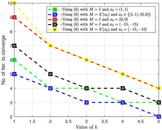
Thus, the comparison shows that the behavior of method (6) is essentially the same as method (5). However, the iterates of method (6) are cheaper to obtain than (5). As observed in Table 1, Table 2, Table 3 and Table 4, the number of iterations required for the proposed methods with k ranging from 3 to 5 closely aligns with those of method (5).

Table 1. The number of iterations needed to achieve tolerance $\epsilon ={10}^{-9}$ (i.e, ($\parallel s_k-s_{k-1}\parallel <{10}^{-9}$)) with initial guess $x_0=(1,1)$, $\lambda =1$ and $\parallel I-{\Lambda }^{\prime }(x_0)\parallel =0.2593<1$.

Method	Iterations	Method	Iterations
Equation (5)	3	Equation (5)	3
Equation (50), $k=1$	6	Equation (55), $k=1$	9
Equation (51), $k=2$	4	Equation (55), $k=2$	7
Equation (52), $k=3$	4	Equation (55), $k=3$	6
Equation (53), $k=4$	3	Equation (55), $k=4$	5
Equation (54), $k=5$	3	Equation (55), $k=5$	4

Table 2. The number of iterations needed to achieve tolerance $\epsilon ={10}^{-9}$ (i.e, ($\parallel s_k-s_{k-1}\parallel <{10}^{-9}$)) with initial guess $x_0=(0,0)$, $\lambda =1$ and $\parallel I-{\Lambda }^{\prime }(x_0)\parallel =0.1<1$.

Method	Iterations	Method	Iterations
Equation (5)	2	Equation (5)	2
Equation (50), $k=1$	5	Equation (55), $k=1$	9
Equation (51), $k=2$	4	Equation (55), $k=2$	7
Equation (52), $k=3$	3	Equation (55), $k=3$	6
Equation (53), $k=4$	3	Equation (55), $k=4$	5
Equation (54), $k=5$	2	Equation (55), $k=5$	4

Table 3. The number of iterations needed to achieve tolerance $\epsilon ={10}^{-9}$ (i.e, ($\parallel s_k-s_{k-1}\parallel <{10}^{-9}$)), where $x_0=(-15,-15)$, $\lambda =1$ and $\parallel I-{\Lambda }^{\prime }(x_0)\parallel =0.2120<1$.

Method	Iterations	Method	Iterations
Equation (5)	3	Equation (5)	3
Equation (50), $k=1$	7	Equation (55), $k=1$	10
Equation (51), $k=2$	5	Equation (55), $k=2$	7
Equation (52), $k=3$	4	Equation (55), $k=3$	6
Equation (53), $k=4$	4	Equation (55), $k=4$	5
Equation (54), $k=5$	3	Equation (55), $k=5$	4

Table 4. The number of iterations needed to achieve tolerance $\epsilon ={10}^{-12}$ (i.e, ($\parallel s_k-s_{k-1}\parallel <{10}^{-12}$)), where $x_0=(-15,-15)$, $\lambda =1$ and $\parallel I-{\Lambda }^{\prime }(x_0)\parallel =0.2120<1$.

Method	Iterations	Method	Iterations
Equation (5)	3	Equation (5)	3
Equation (50), $k=1$	9	Equation (55), $k=1$	12
Equation (51), $k=2$	6	Equation (55), $k=2$	8
Equation (52), $k=3$	5	Equation (55), $k=3$	7
Equation (53), $k=4$	4	Equation (55), $k=4$	6
Equation (54), $k=5$	4	Equation (55), $k=5$	5

The approximated solution is $s^{app}=(-0.1124965854417,-0.0920701967370)$ with the function value error $\parallel \Lambda (s^{app})\parallel =0.3925\times {10}^{-13}$, which is obtained using the initial point $x_0=(-15,-15)$ with the error tolerance $\epsilon ={10}^{-12}$ (i.e, ($\parallel s_k-s_{k-1}\parallel <{10}^{-12}$)). It is observed that with the same tolerance level, one can obtain the mentioned approximated solution for other initial points considered in Table 1 and Table 2.

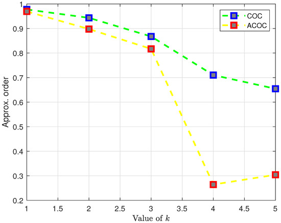
Table 5 and Figure 1 show the results of calculations used to determine the Computational Order of Convergence (COC) and the Approximated Computational Order of Convergence (ACOC), aiming to compare the convergence order of method (6) with the convergence order of method (5).

Table 5. The computational order of convergence and the approximated computational order of convergence, where $x_0=(-15,-15)$, $\epsilon ={10}^{-12}$.

Method	COC	ACOC
Equation (5)	1.0	NA
Equation (50),   $k=1$	0.977468	0.969404
Equation (51), $k=2$	0.943378	0.897736
Equation (52), $k=3$	0.867463	0.816881
Equation (53), $k=4$	0.710293	0.264330
Equation (54), $k=5$	0.654524	0.304212

Figure 1. COC and ACOC using $x_0=(-15,-15)$, $\epsilon ={10}^{-12}$.

Table 5 and Figure 1 demonstrate that the convergence of the proposed methods closely corresponds to the convergence of Newton’s method, particularly for values of k ranging from 4 to 5 with the convergence order closely approximating 2. Furthermore, Figure 2 shows a quick comparison of Table 1, Table 2 and Table 3.

Figure 2. Number of iterations needed to achieve tolerance $\epsilon ={10}^{-9}$.

Example 2.

Let $X=Y={\mathbb{R}}^3$ and $D=S[x^{*},1].$ We study the motion of a particle moving in three dimensions that has started from rest. The mapping Λ is defined on D for $a={(a_1,a_2,a_3)}^T\in {\mathbb{R}}^3$ as:

$$\begin{array}{c}\hfill \Lambda (a)={(a_1,e^{a_2}-1,{\displaystyle \frac{e-1}{2}}{a}_3^2+a_3)}^T.\end{array}$$

(56)

Then, the definition of the derivative according to Fréchet [2,10,13,18,19,20] is given for the mapping Λ:

$${\Lambda }^{\prime }(a)=\left[\begin{array}{ccc}1& 0& 0\\ 0& e^{a_2}& 0\\ 0& 0& (e-1)a_3+1\end{array}\right].$$

The point $x^{*}={(0,0,0)}^T$ solves the equation $\Lambda (a)=0.$ Moreover, ${\Lambda }^{\prime }(x^{*})=I.$ The conditions of Theorem 1 hold provided that $w_0(t)=(e-1)t,w(t)=e^{{\displaystyle \frac{1}{e-1}}}t,{\rho }_0={\displaystyle \frac{1}{e-1}},k=1,\lambda ={\displaystyle \frac{1}{2}}$ and $\delta =(e-1)t.$ Then, by (37), we have $r_1=0.231165,r_2=0.393879,r_3=0.131383=r^{\prime }.$

Example 3.

Let $K[0,1]$ stand as the space of continuous functions mapping the interval $[0,1]$ into the real number system. Let $X=Y=K[0,1]$ and $D=S[x^{*},1]$ with $x^{*}(\xi )=0.$ The operator Λ is defined on $K[0,1]$ as:

$$\Lambda (z)(\xi )=z(\xi )-6{\int }_0^1\xi z{(\tau )}^{3}d\tau .$$

Nonlinear integral equations of the form $\Lambda (z)(\xi )=0$ are of Hemmerstein-type and are used to study the motion problems [5,12,18,19]. Here, the definition of the derivative according to Fréchet gives for the function Λ:

$${\Lambda }^{\prime }(z(w))(\xi )=w(\xi )-18{\int }_0^1\xi \tau z{(\tau )}^{2}w(\tau )d\tau$$

for each $w\in K[0,1].$ Therefore, the conditions are validated, since for $x^{*}=0,M=I,$${\Lambda }^{\prime }(x^{*}(\xi ))=I$, provided that $w_0(t)=18t,w(t)=36t,\delta =18t,\lambda ={\displaystyle \frac{1}{2}},{\rho }_0={\displaystyle \frac{1}{18}}.$ Then, we obtain by (37) that $r_1=0.016615,r_2=0.051081,r_3=0.009570=r^{\prime }.$

7. Concluding Remarks

The Chebyshev method is of R-order three. However, it is computationally expensive because it requires the evaluation of the second derivative of the operator involved at each step of the iteration. By replacing the second derivative in terms of first derivatives, new methods are derived of R-order three. However, the implementation still remains for the new methods, since the inverse of a certain linear operator also needs to be computed. That is why we replace the inverse by a finite sum of linear operators converging to that inverse. The local as well as the semi-local analysis of convergence is studied, relying on the concept of related conditions that control the derivative and majorizing sequences. The sequence generated by the new HCTM are easier to find and essentially converge to the solution as fast as the optimized Chebysehev methods. This fact is also demonstrated by numerical examples. Due to its generality, the methodology of this article can also be applied to other methods with inverses [11,16,19,20,21,22,23]. This is the direction of our future work.

References

- Argyros, I.K.; George, S. On the complexity of extending the convergence region for Traub’s method. J. Complex. 2020, 56, 101423. [Google Scholar] [CrossRef]
- Ben-Israel, A.; Greville, T.N.E. Generalized Inverses: Theory and Applications; John Wiley and Sons: New York, NY, USA, 1974. [Google Scholar]
- Moore, R.H.; Nashed, M.Z. Approximations to generalized inverses of linear operators. SIAM J. Appl. Math. 1974, 27, 1–16. [Google Scholar] [CrossRef]
- Nashed, M.Z. Generalized Inverses and Applications; Academic Press: New York, NY, USA, 1976. [Google Scholar]
- Padcharoen, A.; Kumam, P.; Chaipunya, P.; Shehu, Y. Convergence of inertial modified Krasnoselskii-Mann iteration with application to image recovery. Thai J. Math. 2020, 18, 126–142. [Google Scholar]
- Proinov, P.D.; Petkova, M.D. Local and semilocal Convergence of a family of Multi-point Weierstrass-type Root-Finding Methods. Mediterr. J. Maths. 2020, 17, 107. [Google Scholar] [CrossRef]
- Regmi, S.; Argyros, I.K.; George, S.; Argyros, C.I. Extended Convergence of Three Step Iterative Methods for Solving Equations in Banach Space with Applications. Symmetry 2022, 14, 1484. [Google Scholar] [CrossRef]
- Häubler, W.M. A Kantorovich-type convergence analysis for the Gauss-Newton-method. Numer. Math. 1986, 48, 119–125. [Google Scholar]
- Argyros, I.K.; George, S.; Shakhno, S.; Regmi, S.; Havdiak, M.; Argyros, M.I. Asymptotically Newton-Type Methods without Inverses for Solving Equations. Mathematics 2024, 12, 1069. [Google Scholar] [CrossRef]
- Kantorovich, L.V.; Akilov, G. Functional Analysis in Normed Spaces; Fizmatgiz: Moscow, Russia, 1959; (German translation, Akademie-Verlag: Berlin, Germany, 1964): (English translation (2nd edition), Pergamon Press: London, UK, 1981), (1964). [Google Scholar]
- Ezquerro, J.A.; Hernandez-Veron, M.A. Domains of global convergence for Newtons’s method from auxiliary points. Appl. Math. Lett. 2018, 85, 48–56. [Google Scholar] [CrossRef]
- Ezquerro, J.A.; Hernandez-Veron, M.A. Newton’s Method: An Updated Approach of Kantorovich’s Theory; Birkhauser: Basel, Switzerland, 2017. [Google Scholar]
- Krasnoselskij, M.A. Two remarks on the method of successive approximations. Uspehi Mat. Nauk. 1995, 10, 123–127. (In Russian) [Google Scholar]
- Traub, J.F.; Wozniakowsi, H. Convegence and complexity of Newton iteration for operator equations. J. Assoc. Comput. March. 1979, 26, 250–258. [Google Scholar] [CrossRef]
- Proinov, P.D. New general convergence theory for iterative processes and its applications to Newton- Kantarovich type theorems. J. Complex. 2010, 25, 3–42. [Google Scholar] [CrossRef]
- Ostrowski, A.M. Solution of Equations in Euclidean and Banach Spaces; Academic Press: New York, NY, USA, 1973. [Google Scholar]
- Yamamoto, T. A convergence theorem for Newton-like methods in Banach spaces. Numer. Math. 1987, 51, 545–557. [Google Scholar] [CrossRef]
- Berinde, V. Iterative Approximation of Fixed Points; Springer: New York, NY, USA, 2007. [Google Scholar]
- Deuflhard, P. Newton Methods for Nonlinear Problems. Affine Invariance and Adaptive Algorithms; Springer Series in Computational Mathematics; Springer: Berlin/Heidelberg, Germany, 2004; Volume 35. [Google Scholar]
- Ezquerro, J.A.; Gutierrez, J.M.; Hernandez, M.A.; Romero, N.; Rubio, M.J. The Newton Method: From Newton to Kantorovich. Gac. R. Soc. Mat. Esp. 2010, 13, 53–76. (In Spanish) [Google Scholar]
- Rheinboldt, W.C. A unified convergence theory for a class of iterative process. SIAM J. Numer. Anal. 1968, 5, 42–63. [Google Scholar] [CrossRef]
- Catinas, E. The inexact, inexact perturbed, and quasi-Newton methods are equivalent models. Math. Comp. 2005, 74, 291–301. [Google Scholar] [CrossRef]
- Potra, F.A. Sharp error bounds for a class of Newton-like methods. Lib. Math. 1985, 5, 71–84. [Google Scholar]
Disclaimer/Publisher’s Note: The statements, opinions and data contained in all publications are solely those of the individual author(s) and contributor(s) and not of MDPI and/or the editor(s). MDPI and/or the editor(s) disclaim responsibility for any injury to people or property resulting from any ideas, methods, instructions or products referred to in the content. |
© 2024 by the authors. Licensee MDPI, Basel, Switzerland. This article is an open access article distributed under the terms and conditions of the Creative Commons Attribution (CC BY) license (https://creativecommons.org/licenses/by/4.0/).