Article

The Integrability and Modification to an Auxiliary Function Method for Solving the Strain Wave Equation of a Flexible Rod with a Finite Deformation

by
Adel Elmandouh
1,2,*,
Aqilah Aljuaidan
1 and
Mamdouh Elbrolosy
1,3
1
Department of Mathematics and Statistics, College of Science, King Faisal University, P.O. Box 400, Al-Ahsa 31982, Saudi Arabia
2
Department of Mathematics, Faculty of Science, Mansoura University, Mansoura 35516, Egypt
3
Department of Mathematics, Faculty of Science, Tanta University, Tanta 31527, Egypt
*
Author to whom correspondence should be addressed.
Mathematics 2024, 12(3), 383; https://doi.org/10.3390/math12030383
Submission received: 14 December 2023 / Revised: 20 January 2024 / Accepted: 23 January 2024 / Published: 24 January 2024

Abstract

:
Our study focuses on the governing equation of a finitely deformed flexible rod with strain waves. By utilizing the well-known Ablowita–Ramani–Segur (ARS) algorithm, we prove that the equation is non-integrable in the Painlevé sense. Based on the bifurcation theory for planar dynamical systems, we modify an auxiliary equation method to obtain a new systematic and effective method that can be used for a wide class of non-linear evolution equations. This method is summed up in an algorithm that explains and clarifies the ease of its applicability. The proposed method is successfully applied to construct wave solutions. The developed solutions are grouped as periodic, solitary, super periodic, kink, and unbounded solutions. A graphic representation of these solutions is presented using a 3 D representation and a 2 D representation, as well as a 2 D contour plot.

1. Introduction

To develop fundamental phenomena and implementations, many non-linear physical structures have been connected to non-linear equations in multiple fields, including plasma physics, fluid dynamics, wave propagation, fluid flow, thermodynamics, non-linear networks, optical including fiber, mechanics, and soil stability. In non-linear sciences, as well as many other disciplines of research, non-linearity plays an important role. In addition, recent years have seen increasing attention directed at finding an exact solution for partial non-linear equations. The reason is that the existence of the exact solutions enables the researchers to explain, understand, and have much knowledge required to analyze the properties of physical phenomena described by non-linear partial differential equations. This motivates scholars to introduce new approaches or develop existing ones. In the literature, there are several efficient and trustworthy approaches for exploring analytic solutions. Several effective and trustworthy approaches have been introduced in the literature for finding the analytic solutions such as the homogeneous balance method [1,2], Hirota bilinear method [3,4], the Backlund transformation method [5,6], the inverse scattering method [7,8], Semi-inverse variational principle [9,10], algebraic method [11,12], the first integral method [13], an extended mapping technique [14], the Riccati–Bernoulli sub-ODE and e x p ( G / G ) expansion method [15], the extended exponential function method [16], Lie symmetry analysis [17,18], a modified F-expansion method [19], unified auxiliary equation method [20], three algebraic methods; 1 / G , modified G / G 2 and new extended direct algebraic methods [21], the blackuctive perturbation method [22], bifurcation theory [23,24,25,26,27,28], and for other several methods, see, e.g., [29,30,31,32,33,34,35].
It is well known that non-linear elastic waves have also been used to address a variety of technological matters. There are various sources of non-linearities in solid structures, such as geometrical and physical non-linearities, kinetic non-linearities, and boundary constraints. Solitary and shock wave solutions occur when non-linearity interacts with dispersion or dissipation effects to produce steady traveling wave solutions. Increasingly, problems involving non-linearity are being analyzed and solved qualitatively using the non-linear evolution equation. As a consequence, we analyze some dynamic analysis of
2 u t 2 c 0 2 2 u x 2 = 2 x 2 c 0 2 2 ( 3 u 2 + u 3 ) + ν 2 R 2 2 2 u t 2 c 1 2 2 u x 2 ,
which is called the strain wave equation [36]. The longitudinal wave velocity and shear wave velocity are denoted by c 0 = E ρ , c 1 = μ ρ , respectively. μ , ρ , E, and u ( x , t ) refer to the material shear modulus, the rod density per unit volume, elastic modulus, and distribution of the displacement at x , t , respectively. The model in Equation (1) explains a double non-linear wave equation for an elastic circular-rod wave-guide. It involves the axial displacement gradient and accounts for the transverse Poisson effect, which causes the longitudinal and shear waves to propagate together. Hamilton’s principle of least action is applied to derive the model [36]. In [37], the authors described the non-linear dispersive dissipative evolution of strain waves in a solid with certain limiting conditions. They constructed a bounded periodic solution and a kink solution. In [36], the authors constructed a solitary wave solution for the governed equation by applying the hyperbolic secant function finite expansion method. In [38], the authors applied the Jacobi elliptic sine function and the third kind of Jacobi elliptic function, finite expansion, to obtain exact periodic solutions of double non-linearity and double dispersion wave equations (cubic non-linear item) and corresponding truncation equations (square non-linear items) of the circular-rod-waveguide. In [39], the authors applied qualitative analysis and utilized the principle of homogeneous balance to solve the governed equation with the Jacobi elliptic function expansion method to construct solitary wave solutions, and they also illustrate that the existence of shock wave solutions is possible under certain conditions. Solely, both solitary and shock wave solutions are found which are commonly not capable of producing an exact periodic solution. Shock, periodic, and solitary solutions of the derived equation have been found by utilizing the Jacobi elliptic function expansion method [40]. Based on the bifurcation analysis, some new solutions, dependence on the initial conditions, influence on the physical parameters, and the existence of quasi-periodic solution are investigated by the current authors [41].
As a result, Section 2 includes the study of the integrability of the governing equation via Painlevé analysis. Section 3 presents the proposed method for developing traveling wave solutions for non-linear partial differential equations, based on bifurcation analysis, and an algorithm to demonstrate its applicability. By applying the newly proposed technique to the governing equation, we obtain some new wave solutions in Section 4. By presenting 3D and 2D representations as well as 2D contours, these solutions are clarified graphically in Section 5. The results are summarized in Section 6.

2. Painlevé Analysis

The integrability of Equation (1) is examined in the current section by utilizing the Painlevé singularity analysis. The ARS algorithm is a powerful technique to study the integrability of partial differential equations [42]. To have a self-contained article, we introduce briefly the ARS algorithm in Appendix A. It is applied successfully in several works, see e.g., [43,44,45,46]. We prove the next theorem
Theorem 1. 
The strain wave Equation (1) of a flexible rod with a finite deformation is not integrable in Painlevé sense.
Proof. 
The generalized Laurent series for the independent variable u ( x , t ) in the neighborhood of a non-characteristic singular manifold ψ ( x , t ) with ψ t 0 and ψ x 0 admits the form
u ( x , t ) = ψ p ( x , t ) j = 0 u j ( x , t ) ψ j ( x , t ) ,
where u 0 ( x , t ) 0 and p Z are to be calculated. The leading order term is postulated to be
u ( x , t ) = u 0 ( x , t ) ψ p ( x , t ) .
Inserting Equation (2) into Equation (1), p is calculated by balancing the most dominate terms. Hence, we find p = 1 . The coefficient of the leading term u 0 ( x , t ) , which is determined by comparing the coefficient of ψ 5 , is given by
u 0 ( x , t ) = ± R ν c 0 2 ( c 1 2 ψ x 2 ψ t 2 ) .
The resonances, which are the powers of ψ at which the free functions appear in the Laurent series, are determined by plugging the expression
u ( x , t ) = u 0 ( x , t ) ψ 1 ( x , t ) + u r ( x , t ) ψ r 1 ( x , t ) ,
into Equation (1) and equating the coefficient of ψ ( x , t ) r 5 to zero, we get
R 2 ν 2 u r ( r + 1 ) ( r 3 ) ( r 4 ) 2 ψ x 2 ( c 1 2 ψ x 2 ψ t 2 ) = 0 ,
where u 0 ( x , t ) is eliminated by Equation (5). It is clear that u r are arbitrary functions if r = 1 , 3 , 4 , 4 . Notice that there is always a resonance r = 1 which corresponds to the arbitrariness of the singular manifold ψ ( x , t ) . As the Equation (1) admits more resonances at j = 4 , 4 than the required arbitrary functions, we conclude that Equation (1) fails to satisfy the Painlevé test. Hence, the theorem is proved. □

3. Proposed Method

Due to the governed equation for the elastic rod with a finite deformation, Equation (1) being non-integrable in the Painlevé sense, quasi-analytical methods or numerical analysis are needed to discover special solutions such as wave solutions. This motivate us to develop and modify the current methods to be more systematic and effective for constructing wave solutions for non-linear partial differential equations. In this section, we perform a combination of the bifurcation theory [47] and the auxiliary equation method [48]. In a comparison with previous methods [36,37,38,39,40], this combination will lead to some significant advantages as we clarify below.

3.1. Method Description

Considering that the general form of the partial differential equation takes the form:
K ( u , u t , u x , u t t , u x t , u x x , ) = 0 .
We employ the transformation
u ( x , t ) = φ ( ξ ) , ξ = k ( x ω t ) ,
where ξ is the wave number while w and k are constants characterizing the wave speed and wave number respectively. Inserting the transformation (8) into Equation (7), we obtain an ordinary differential equation
P ( φ , k ω φ , k φ , k 2 ω 2 φ , k 2 ω φ , k 2 φ , ) = 0 ,
where primes refer to derivatives with respect to the wave variable ξ . This equation is called an reduced equation. We assume Equation (9) has a solution in the form
φ ( ξ ) = j = 0 N a j τ ( ξ ) j ,
where a j are constants required to be determined and N Z + is calculated by balancing the highest power of the non-linear term with the highest order derivative terms in Equation (9), besides our assumption that τ ( ξ ) satisfies the auxiliary differential equation
τ = β ( τ 4 δ τ 2 ) + 2 e ,
where β , δ , e are arbitrary constants. Thus, the key to constructing a solution for the main partial differential Equation (7) is to find a solution for the reduced Equation (9). Thus, separating the variables of Equation (11) gives the one-differential form
d τ P 4 ( τ ) = d ξ ,
where
P 4 ( τ ) = β ( τ 4 δ τ 2 ) + 2 e .
The parameters β , δ , e must fall within a suitable range for the integration of both sides of Equation (12). There are various ways to accomplish this, including the discriminating approach and bifurcation. The bifurcation theory is more significant because it enables us to specify the kind of solutions before constructing them through type of the phase orbits. For instance, the existence of periodic orbits, homoclinic orbits, and heteroclinic orbits indicates the presence of periodic, solitary and kink (or anti-kink) solutions. It has been applied successfully in several works, see e.g., [49,50,51] as well as being applied to find the solutions for the stochastic partial differential equation [52,53] and investigating the chaotic behavior for perturbed partial differential equations containing perturbed periodic term [54]. In this work, we apply the bifurcation theory [47] by using the Hamiltonian concepts to find the solution of Equation (11) that can be expressed as
1 2 τ 2 β 2 ( τ 4 δ τ 2 ) = e .
Equation (14) is equivalent to the conserved quantity for a one-dimension conservative Hamiltonian system which is derived from the Hamiltonian function
H = 1 2 τ 2 + U ( τ ) ,
where U is the potential function
U ( τ ) = β 2 ( τ 4 δ τ 2 ) .
Notice that the constant e does not appear in the potential function (16) and moreover, it enters the Hamiltonian (15) linearly. Hence, it can be taken as the energy constant for the Hamiltonian (15) [55,56].
Now, we are going to apply the bifurcation analysis for the Hamiltonian (15). Firstly, we find the equilibrium points for the Hamiltonian (15) which appear as the critical points for the potential function (16), i.e., they are ( τ 0 , 0 ) , where τ 0 is a solution for U ( τ 0 ) = β τ ( 2 τ 0 3 δ τ ) = 0 . Thus, if δ > 0 , there exist three equilibrium points E 0 = ( 0 , 0 ) , E 1 , 2 = ( ± δ 2 , 0 ) while if δ < 0 , there is a single equilibrium point E 0 = ( 0 , 0 ) . The equilibrium point can be assorted according to whether it is either the maximum or minimum point for the potential function (16). Therefore, we calculate
U ( E 0 ) = β δ , U ( E 1 , 2 ) = 2 β δ .
Assuming the condition of the equilibrium point is met, we find:
(a)
If δ < 0 , the Hamiltonian (15) has a single equilibrium point E 0 = ( 0 , 0 ) which is either center point if β < 0 or saddle point if β > 0 . The phase portrait for these cases are depicted in Figure 1a,b.
(b)
If δ > 0 , the Hamiltonian (15) owns three equilibrium points E 0 , 1 , 2 . For β > 0 , E 0 is a center point while E 1 , 2 are saddle points while for β < 0 , the two equilibrium points E 1 , 2 are center and E 0 is saddle point. The phase portrait for both cases of β is depicted by Figure 1c,d.
The value of the conserved quantity (14) at the equilibrium points are
e 0 = e ( E 0 ) = 0 , e 1 = e ( E 1 , 2 ) = β δ 2 8 .
Depending on the bifurcation conditions on the parameters β , δ , e , we can integrate both sides of Equation (12) to construct the possible solutions for the auxiliary Equation (9). These solutions are accumulated in Table 1, Table 2 and Table 3 to avoid ambiguity.
  • Equation (13) can be expressed as
    P 4 ( τ ) = β ( τ 2 r 1 2 ) ( τ 2 r 2 2 ) ,
    where
    r 1 2 = β δ + β 2 δ 2 8 β e 2 β , r 2 2 = β δ β 2 δ 2 8 β e 2 β .
The zeros of P 4 ( τ ) are then τ = ± r 1 2 and τ = ± r 2 2 which may be real or complex according to the values of the parameters β , δ and e.
We sum up our proposed method in the following algorithm to demonstrate how easily it can be applied.

Algorithm

An algorithm is presented to demonstrate the applicability of the proposed method. We consider a non-linear partial differential equation in the form (7). To construct possible wave solutions, we follow the steps shown below:
  • Step 1: Applying the wave transformation (8) to Equation (7), we obtain an ordinary differential Equation (9) which is the reduced equation.
  • Step 2: Assuming the reduced Equation (9) has a solution
    φ ( ξ ) = j = 0 N a j τ ( ξ ) j ,
    where τ ( ξ ) is a solution of the auxiliary equation
    τ ( ξ ) = β ( τ 4 δ τ 2 ) + 2 e .
  • Step 3: Determining the positive integer N by balancing the highest power of the non-linear term with the highest order derivative terms in the auxiliary Equation (9). After some calculations, the highest order derivative term φ and highest power of the non-linear term φ m with positive integer m > 1 , in the reduced equation are given by
    O ( φ ) = N + 2 , O ( φ m ) = m N .
Equating the last expression, we obtain
N = 2 m 1 .
Because N is a positive integer, we have two possible cases:
  • Case I: If m = 2 , 3 , then we have N = 2 , 1 , respectively, and go directly to the next step.
  • Case II: If m 4 , we perform the transformation φ ( ξ ) = G ( ξ ) 2 / ( m 1 ) to the reduced equation and assume its solution admits the form (21), i.e.,
    G ( ξ ) = j = 0 N a j τ ( ξ ) j .
    Then, go to the next step.
  • Step 4: Inserting the assumed solution (21) in Equation (7), using the Equation (22), and equating all the coefficients of all powers of τ in the resulting polynomial to zero, we obtain a non-linear algebraic system in a j and the physical parameters of the problem.
  • Step 5: Solving the last system to find a j in terms of the physical parameters and utilizing Table 1, Table 2 and Table 3 to construct the solutions for the reduced equation and consequently, to the non-linear partial differential equation under consideration.
The proposed method has many advantages as a result of its dependence on bifurcation theory in its formulation. This is illustrated in the following:
(a)
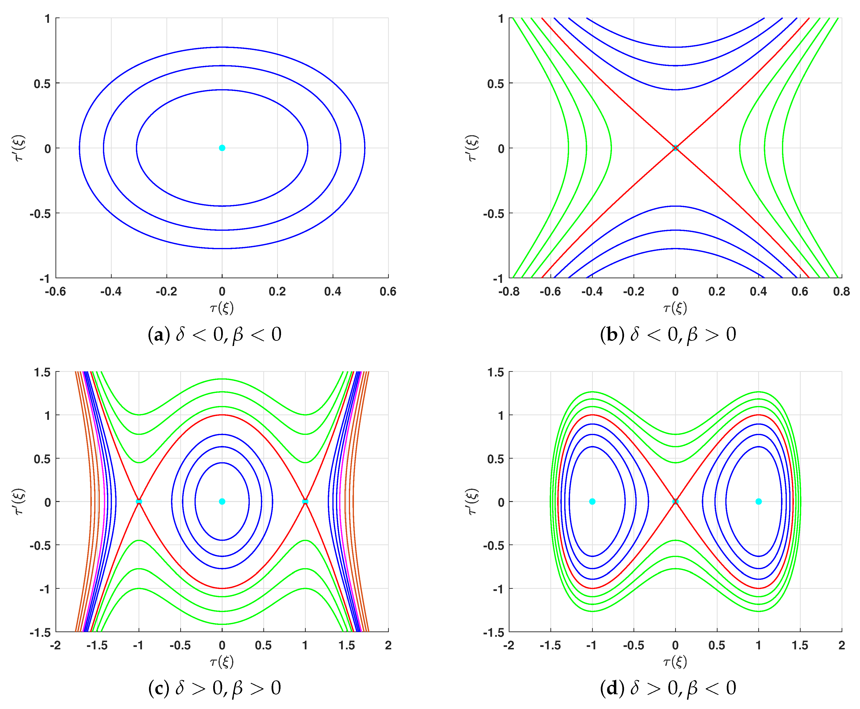
It is utilized only to construct real (not complex) wave solutions for the given NPDE, because these solutions are constructed by integrating the conserved quantities along all possible intervals of real wave propagation. Moreover, the entering of the concept of the interval of real wave propagation intervals enables us to construct all possible wave solutions that are completely different from mathematical and physical points of view. Let us clarify this point. For the choice δ > 0 , β > 0 and e ] e 0 , e 1 [ , there are two solutions. One of them is periodic as illustrated by row 2 in Table 1 while the other is unbounded as outlined by row 6 in Table 3 row. Thus, we have two completely different solutions from mathematical and physics points of view for the same conditions of the parameters.
(b)
It enables us to know in advance the types of solutions. For example in Table 1, the first three cases are periodic solutions because they are related to periodic orbits in phase portrait while the fourth case is a super periodic solution since it corresponds to the super periodic orbit, see Figure 1. Therefore, the assumed solution can be viewed as a combination of periodic solutions or super periodic solutions, respectively. For this reason, we know the obtained solution will be periodic or supper periodic.
(c)
Thanks to employing bifurcation analysis, we were able to isolate all possible bounded solutions that are required and significant in real-world problems.

4. Application

The current section aims to clarify how to apply the proposed method by following the introduced algorithm. Based on the first step, we insert the wave transformation (8) into the Equation (1), and we get
( ω 2 c 0 2 ) d 2 u d ξ 2 c 0 2 2 d 2 d ξ 2 ( 3 u 2 + u 3 ) ν 2 R 2 k 2 2 d 2 d ξ 2 [ ( ω 2 c 1 2 ) d 2 u d ξ 2 ] = 0 .
Integrated Equation (25) twice with respect to ξ and neglecting the integration constants gives
d 2 u d ξ 2 = c u + 3 a u 2 + a u 3 ,
where
c = 2 ( ω 2 c 0 2 ) ν 2 R 2 k 2 ( ω 2 c 1 2 ) and a = c 0 2 ν 2 R 2 k 2 ( ω 2 c 1 2 ) .
According to the second step, we postulate Equation (26) has a solution in the form
u ( ξ ) = j = 0 N a j τ ( ξ ) j ,
where a j is a constant required to be determined besides τ ( ξ ) satisfies a first order differential Equation (22). Following Equation (24), we get N = 1 . Hence, the assumed solution becomes
u ( ξ ) = a 0 + a 1 τ ( ξ ) .
Now, we are going to determine the constants a 0 , a 1 , β , δ , e in terms of the physical parameters. Inserting the expression (29), taking into account the Equation (22), and equating the coefficient of all powers of τ ( ξ ) to zero, we get the following algebraic system
a 1 ( 2 β a a 1 2 ) = 0 , a a 1 2 ( a 0 + 1 ) = 0 , a 1 [ c + β δ + 6 a a 0 + 3 a a 0 2 ] = 0 , a 0 [ c + 3 a a 0 + a a 0 2 ] = 0 .
The only working solution of the algebraic system (30) is
a = c 2 , a 0 = 1 , δ = a β , a 1 = 2 β a ,
where a β > 0 is a condition for the solution (29) to be real. Thus, we consider the following cases:
  • Case A: For a > 0 , we have β > 0 and consequently δ > 0 . For bounded solutions, the only working case is Case 2 in Table 1. Thus, Equation (1) has the following solution if e ] 0 , a 8 β [
    u ( x , t ) = 1 ± 2 β a r 2 sn ( r 1 β k ( x ω t ) , r 1 r 2 ) .
The solution (31) is a new periodic solution for Equation (1). For Table 2, the first case in which δ > 0 , β > 0 is the only working case in this table. Thus, Equation (1) has the solution
u ( x , t ) = 1 ± 2 β a δ 2 tan h δ β 2 k ( x ω t ) .
The solution (32) is a new kink solution for Equation (1). For unbounded wave solutions, the working cases in Table 3 are Cases 4–7 and they are classified according to values of e. Thus, we have
1.
If e < 0 , Equation (1) owns the following new solution
u ( x , t ) = 1 ± r 1 2 β a nc ( β ( r 1 2 r 2 2 ) k ( x ω t ) , r 2 2 r 2 2 r 1 2 ) .
2.
If e = 0 , we introduce a novel solution for Equation (1) in the form
u ( x , t ) = 1 ± 2 β δ a sec δ β k ( x ω t ) .
3.
If e ] 0 , β δ 2 8 [ , the governing Equation (1) has a new solution
u ( x , t ) = 1 ± r 1 2 β a dc ( r 1 k β ( x ω t ) , r 2 r 1 ) .
4.
If e > β δ 2 8 , then
u ( x , t ) = 1 ± r 1 2 β a nd ( | r 1 | β ξ , k 3 ) sc ( | r 1 | β ξ , k 3 ) .
is a new solution for Equation (1).
  • Case B: For the choice a < 0 , β must be negative, i.e., β < 0 and hence δ > 0 . Therefore, the only working cases in Table 1 are Case 3 and Case 4. Let us consider them individually.
1.
If e ( a 8 β , 0 ) , Equation (1) has a new solution in the form
u ( x , t ) = 1 + 2 β a r 2 dn ( r 2 β k ( x ω t ) , 1 r 1 2 r 2 2 ) .
2.
If e ] 0 , [ , then Equation (1) has the solution
u ( x , t ) = 1 + 2 β a r 2 cn ( k β ( r 2 2 r 1 2 ) ( x ω t ) , r 2 r 2 2 r 1 2 ) .
As we see also in Table 2, the only working case is the second one. Hence, if e = e 0 = 0 Equation (1) has the solution
u ( x , t ) = 1 ± 2 β δ a sec h δ β k ( x ω t ) ,
which is a new solitary wave solution for Equation (1).

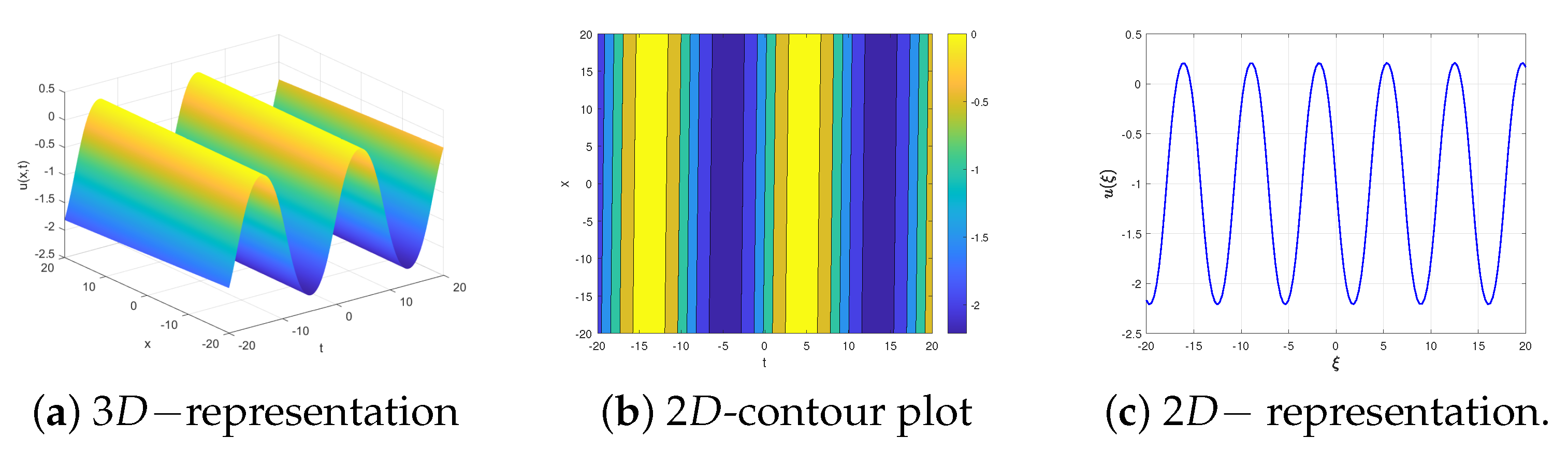
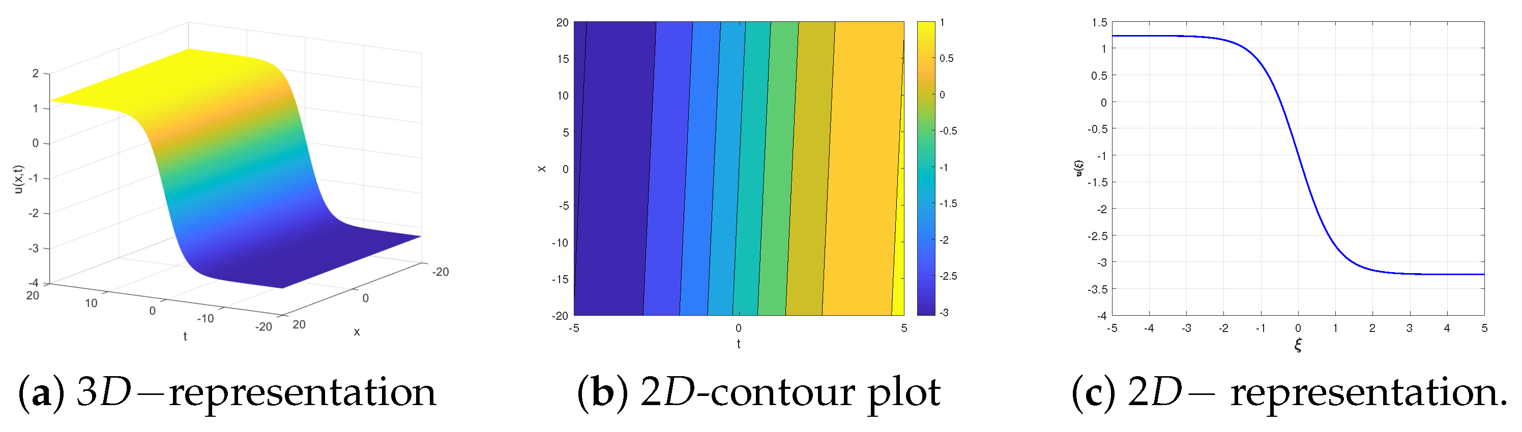
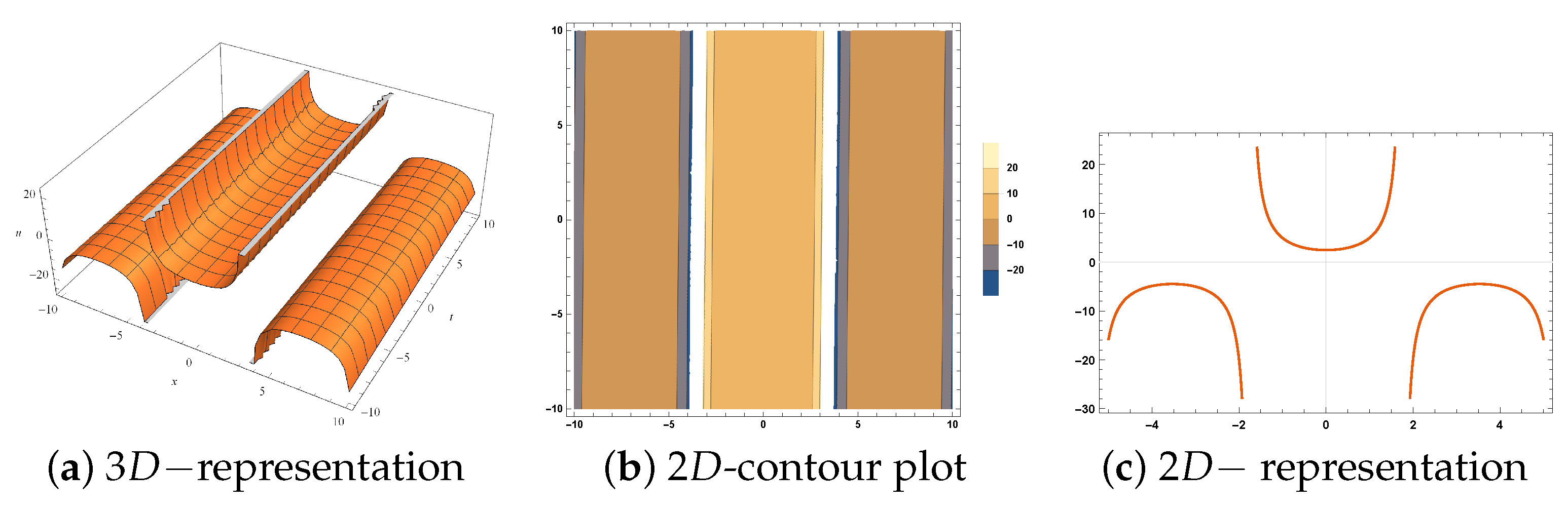
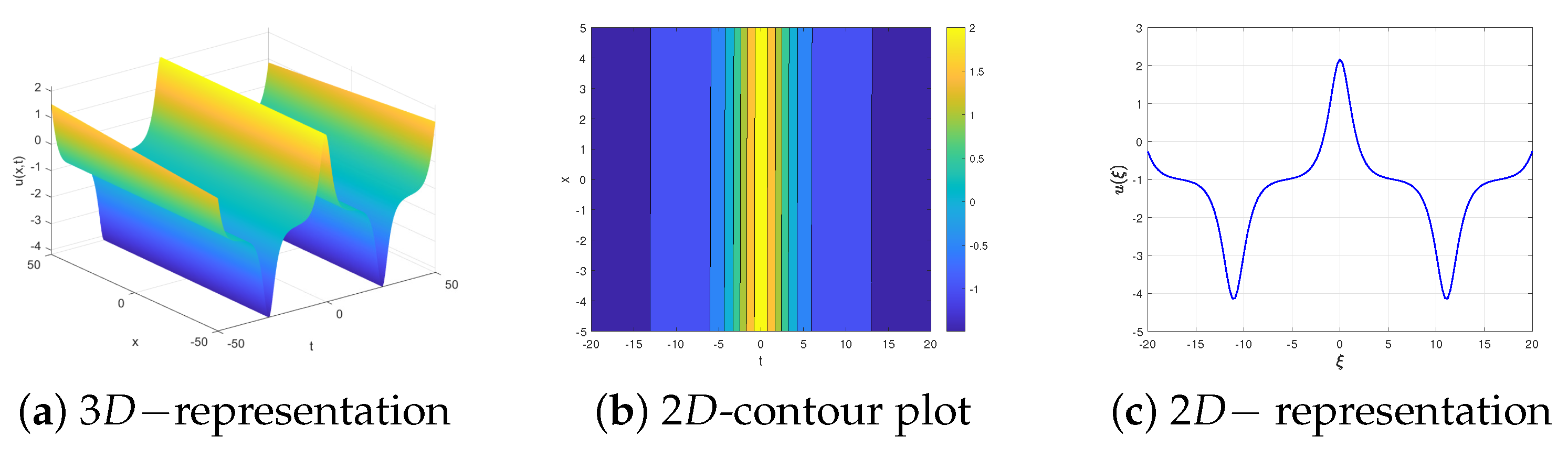
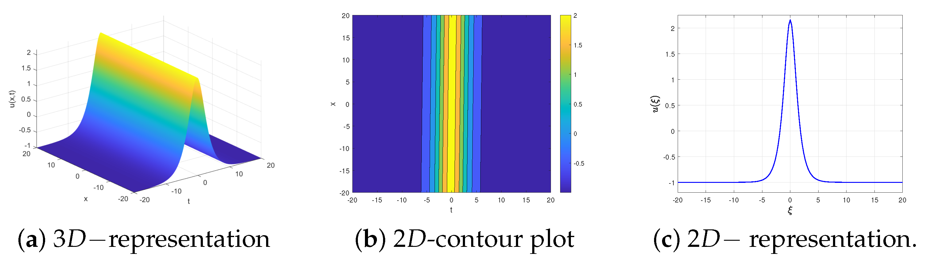
5. Physical Interpretations

This section aims to illustrate the obtained solutions graphically by introducing 2 D and 3 D graphics, as well as the contour plots for different kinds of the obtained solutions using Matlab and Mathematica programs. We presume that k = 0.1 , ω = 0.3 in all the subsequent computations.
For real solutions, the selected values of a and β must satisfy the condition a β > 0 and consequently δ > 0 . Hence, there are two possible choices of the two parameters, a and β . They are either a > 0 , β > 0 or a < 0 , β < 0 . Let us consider each of them individually:
Firstly, We consider the solutions introduced in Case A. We assume c = 0.8 and β = 1 , and so a = 0.4 and δ = 0.4 . For these values, we have e 1 = 0.02 and the roots of the quartic polynomial (13) satisfy r 1 2 = 0.2 0.08 and r 2 2 = 0.2 + 0.08 . By taking e = 0.01 , the periodic solution (31) for the Equation (1) is depicted in Figure 2. It also clarifies one of the advantages of the proposed method, which is the ability to determine the type of solution before it is constructed, simply by knowing the parameters.
Preserving the same values for c, and β and choosing different values of e, we will construct several solutions which are completely different from mathematical and physical points of views.
1.
For e = e 1 = 0.02 , Figure 3 shows the graphical representation of the solution (32) by presenting the 3 D and 2 D representation besides the 2 D contour plot.
2.
For e = 0.5 ] , 0 [ , we have r 1 2 = 0.2 1.1 and r 2 2 = 0.2 + 1.1 . Hence, the quartic polynomial (13) has two real roots and two imaginary roots. Therefore, the solution (33) can be visualized by Figure 4 which includes the 3 D and 2 D graphical representation of the solution in addition to the 2 D contour plot.
Secondly, we consider the solutions which are presented in Case B. We postulate c = 0.8 and β = 1 , so, a = 0.4 and δ = 0.4 . Depending on the value of e, the possible solutions can be constructed.
1.
If e = 0.001 ( 0 , ) , Equation (1) admits the super periodic solution (38) which is illustrated by Figure 5.
2.
If e = 0 , Equation (1) has the one soliton solution (39) which is clarified by Figure 6.

6. Conclusions

The current work focused on studying the governing equation describing the strain wave equation of a flexible rod with a finite deformation. Based on the singularity analysis, we have proved the non-integrability of the governing equation. We present a new modification to the auxiliary equation method for constructing wave solutions for a large class of non-linear partial differential equations. The formulation of this method relies on the bifurcation theory for planar integrable systems. The formulation procedures furnish more effective advantages for the new method. These advantages are summarized as:
(a)
It is only applied to construct real (not complex) wave solutions for a large class of partial differential equations by integrating the conserved quantities along the intervals of real wave propagation. Moreover, with the same conditions on the parameters and different intervals of real wave propagation, distinct solutions from mathematical and physical points of view are constructed. For instance, for the choice δ > 0 , β > 0 and e ] e 0 , e 1 [ , there are two solutions. One of them is periodic as illustrated by row 2 in Table 1, while the other is unbounded as outlined by row 6 in Table 3 row.
(b)
It enables us to know the kinds of solutions before establishing them.
(c)
We can isolate all bounded wave solutions, which is useful in real applications.
This method has been applied to the governing equation aiming to illustrate its applicability and effectiveness to present new solutions for the governing equation. Some novel wave solutions that are assorted into periodic, super periodic, kink, and solitary wave solutions have been introduced. By introducing 2 D , 3 D , and contour plots, some of these solutions are graphically clarified.

Author Contributions

Conceptualization, A.E. and M.E.; methodology, A.E.; software, M.E.; validation, A.A., A.E. and M.E.; formal analysis, A.E.; investigation, M.E.; resources, A.A.; writing original draft preparation, A.A.; writing review and editing, M.E.; supervision, A.E. and M.E.; funding acquisition, A.A. All authors have read and agreed to the published version of the manuscript.

Funding

This work was supported by the Deanship of Scientific Research, Vice Presidency for Graduate Studies and Scientific Research, King Faisal University, Saudi Arabia [Grant No. 5640].

Data Availability Statement

Data are contained within the article.

Acknowledgments

The authors would like to thank the Deanship of Scientific Research, Vice Presidency for Graduate Studies and Scientific Research, King Faisal University, Saudi Arabia for supporting this work.

Conflicts of Interest

The authors declare no conflict of interest.

Appendix A

In this appendix, ARS algorithm is briefly displayed. Consider a non-linear partial differential equation in the form:
L ( u t , u S , u S S , u S S S , ) = 0 ,
where L and u are a polynomial and a complex-valued function depending on the two variables S , t , respectively. This appendix provides a brief description of Painlevé analysis. Painlevé analysis is employed to determine whether the given Equation (A1) is integrable or not. The solution of Equation (A1) is assumed as Laurent series
u ( t , S ) = ϕ p i = 0 u i ( t , s ) ϕ i ( t , S ) ,
where u 0 0 and p is a negative integer needed to be found. We follow the ARS- algorithm that can be outlined in the subsequent steps [58]:
  • Step 1 (Dominate behavior): The leading order term in Laurent series (A2) is assumed to be
    u = u 0 ϕ p .
Inserting the expression into Equation (A1), and balancing the dominant terms, we found the value of p. The coefficient of leading term u 0 is calculated by inserting the Laurent series with the obtained value of p into Equation (A1) and equating the coefficient of the leading term in the obtained equation, we obtain an equation determining u 0 .
  • Step 2 (Resonances): The resonances are defined as the powers at which the arbitrary functions appear in the Laurent series. The resonance can be determined by inserting
    u ( t , S ) = u 0 ϕ p + i = 1 u i ( t , S ) ϕ r + p ,
    into Equation (A1) and comparing different powers of ϕ . Notice that all the resonances are non-negative integers except the resonance r = 1 which refers to the arbitrariness of ϕ . Additionally, the resonance r = 0 indicates the coefficient u 0 of the leading term is arbitrary. If all the values of resonances are non-negative except r = 1 , we are going to the next step.
  • Step 3 (Compatibility conditions): This step aims to check the existence of a sufficient number of arbitrary functions in the Laurent series (A2). This can be performed by inserting the expression
    u ( t , S ) = ϕ p i = 0 r m a x u i ( t , S ) ϕ i ( t , S ) ,
    into Equation (A1) and testing the existence of arbitrary functions corresponding to the obtained resonances in Step 2, where r m a x is the largest value of the resonances. If the compatibility conditions are satisfied then, the given partial differential equation has Painlevé property. Consequently, it is integrable in Painlevé sense, or sometimes it is named Painlevé integrable.

References

  1. Wang, M.; Zhou, Y.; Li, Z. Application of a homogeneous balance method to exact solutions of non-linear equations in mathematical physics. Phys. Lett. A 1996, 216, 67–75. [Google Scholar] [CrossRef]
  2. Elsherbeny, A.M.; Mirzazadeh, M.; Akbulut, A.; Arnous, A.H. Optical solitons of the perturbation Fokas–Lenells equation by two different integration procedures. Optik 2023, 273, 170382. [Google Scholar] [CrossRef]
  3. Yin, T.; Xing, Z.; Pang, J. Modified Hirota bilinear method to (3+1)-D variable coefficients generalized shallow water wave equation. Nonlinear Dyn. 2023, 87, 2529–2540. [Google Scholar] [CrossRef]
  4. Biswas, S.; Ghosh, U.; Raut, S. Construction of fractional granular model and bright, dark, lump, breather types soliton solutions using Hirota bilinear method. Chaos Solitons Fractals 2023, 172, 113520. [Google Scholar] [CrossRef]
  5. Vakhnenko, V.; Parkes, E.; Morrison, A. A Bäcklund transformation and the inverse scattering transform method for the generalised Vakhnenko equation. Chaos Solitons Fractals 2003, 17, 683–692. [Google Scholar] [CrossRef]
  6. Fan, F.C.; Xu, Z.G.; Shi, S.Y. Soliton, breather, rogue wave and continuum limit for the spatial discrete Hirota equation by Darboux–Bäcklund transformation. Nonlinear Dyn. 2023, 111, 10393–10405. [Google Scholar] [CrossRef]
  7. Ali, M.R.; Khattab, M.A.; Mabrouk, S. Optical soliton solutions for the integrable Lakshmanan-Porsezian-Daniel equation via the inverse scattering transformation method with applications. Optik 2023, 272, 170256. [Google Scholar] [CrossRef]
  8. Ali, M.R.; Khattab, M.A.; Mabrouk, S. Travelling wave solution for the Landau-Ginburg-Higgs model via the inverse scattering transformation method. Nonlinear Dyn. 2023, 111, 7687–7697. [Google Scholar] [CrossRef]
  9. He, C.H.; Liu, C. Variational principle for singular waves. Chaos Solitons and Fractals 2023, 172, 113566. [Google Scholar]
  10. Wang, Y.; Gepreel, K.A.; Yang, Y.J. Variational principles for fractal Boussinesq-like B (m, n) equation. Fractals 2023, 31, 1–8. [Google Scholar] [CrossRef]
  11. Arshad, M.; Seadawy, A.R.; Lu, D. Elliptic function and solitary wave solutions of the higher-order non-linear Schrödinger dynamical equation with fourth-order dispersion and cubic-quintic non-linearity and its stability. Eur. Phys. J. Plus 2017, 132, 371. [Google Scholar] [CrossRef]
  12. Arshad, M.; Seadawy, A.; Lu, D.; Wang, J. Travelling wave solutions of Drinfel’d–Sokolov–Wilson, Whitham–Broer–Kaup and (2+1)-dimensional Broer–Kaup–Kupershmit equations and their applications. Chin. J. Phys. 2017, 55, 780–797. [Google Scholar] [CrossRef]
  13. Rehman, H.U.; Awan, A.U.; Allahyani, S.A.; Tag-ElDin, E.M.; Binyamin, M.A.; Yasin, S. Exact solution of paraxial wave dynamical model with Kerr Media by using ϕ6 model expansion technique. Results Phys. 2022, 42, 105975. [Google Scholar] [CrossRef]
  14. Seadawy, A.R.; Arshad, M.; Lu, D. Dispersive optical solitary wave solutions of strain wave equation in micro-structured solids and its applications. Phys. Stat. Mech. Its Appl. 2020, 540, 123122. [Google Scholar] [CrossRef]
  15. El-Ganaini, S. Solitons and other solutions to a new coupled non-linear Schrodinger type equation. J. Egypt. Math. Soc. 2017, 25, 19–27. [Google Scholar] [CrossRef]
  16. Kumar, S.; Kumar, A.; Wazwaz, A.M. New exact solitary wave solutions of the strain wave equation in microstructured solids via the generalized exponential rational function method. Eur. Phys. J. Plus 2020, 135, 870. [Google Scholar] [CrossRef]
  17. Jadaun, V.; Kumar, S. Lie symmetry analysis and invariant solutions of (3+1)-dimensional Calogero–Bogoyavlenskii–Schiff equation. Nonlinear Dyn. 2018, 93, 349–360. [Google Scholar] [CrossRef]
  18. Tu, J.M.; Tian, S.F.; Xu, M.J.; Zhang, T.T. On Lie symmetries, optimal systems and explicit solutions to the Kudryashov–Sinelshchikov equation. Appl. Math. Comput. 2016, 275, 345–352. [Google Scholar] [CrossRef]
  19. Seadawy, A.R.; Ali, A.; Baleanu, D.; Althobaiti, S.; Alkafafy, M. Dispersive analytical wave solutions of the strain waves equation in microstructured solids and Lax’fifth-order dynamical systems. Phys. Scr. 2021, 96, 105203. [Google Scholar] [CrossRef]
  20. Ali, K.K.; Tarla, S.; Ali, M.R.; Yusuf, A.; Yilmazer, R. Physical wave propagation and dynamics of the Ivancevic option pricing model. Results Phys. 2023, 52, 106751. [Google Scholar] [CrossRef]
  21. Siddique, I.; Mehdi, K.B.; Jaradat, M.M.; Zafar, A.; Elbrolosy, M.E.; Elmandouh, A.A.; Sallah, M. Bifurcation of some new traveling wave solutions for the time–space M-fractional NEW equation via three altered methods. Results Phys. 2022, 41, 105896. [Google Scholar] [CrossRef]
  22. Rahman, T.; Tarofder, S.; Orani, M.; Akter, J.; Mamun, A. (3+1)-dimensional cylindrical dust ion-acoustic solitary waves in dusty plasma. Results Phys. 2023, 53, 106907. [Google Scholar] [CrossRef]
  23. Elbrolosy, M.; Elmandouh, A. Bifurcation and new traveling wave solutions for (2+1)-dimensional non-linear Nizhnik–Novikov–Veselov dynamical equation. Eur. Phys. J. Plus 2020, 135, 533. [Google Scholar] [CrossRef]
  24. Elbrolosy, M.; Elmandouh, A. Construction of new traveling wave solutions for the (2+1) dimensional extended Kadomtsev-Petviashvili equation. J. Appl. Anal. Comput. 2022, 12, 533–550. [Google Scholar] [CrossRef]
  25. Elbrolosy, M.; Elmandouh, A. Dynamical behaviour of nondissipative double dispersive microstrain wave in the microstructured solids. Eur. Phys. J. Plus 2021, 136, 955. [Google Scholar] [CrossRef]
  26. Elmandouh, A. Integrability, qualitative analysis and the dynamics of wave solutions for Biswas–Milovic equation. Eur. Phys. J. Plus 2021, 136, 638. [Google Scholar] [CrossRef]
  27. Elbrolosy, M. Qualitative analysis and new soliton solutions for the coupled non-linear Schrödinger type equations. Phys. Scr. 2021, 96, 125275. [Google Scholar] [CrossRef]
  28. Elmandouh, A.; Elbrolosy, M. Integrability, variational principal, bifurcation and new wave solutions for Ivancevic option pricing model. J. Math. 2022, 2, 3. [Google Scholar]
  29. El-Dessoky, M.; Elmandouh, A. Qualitative analysis and wave propagation for Konopelchenko-Dubrovsky equation. Alex. Eng. J. 2023, 67, 525–535. [Google Scholar] [CrossRef]
  30. Adeyemo, O.D.; Khalique, C.M.; Gasimov, Y.S.; Villecco, F. Variational and non-variational approaches with Lie algebra of a generalized (3+1)-dimensional non-linear potential Yu-Toda-Sasa-Fukuyama equation in Engineering and Physics. Alex. Eng. J. 2023, 63, 17–43. [Google Scholar] [CrossRef]
  31. Wang, K. Exact travelling wave solution for the local fractional Camassa-Holm-Kadomtsev-Petviashvili equation. Alex. Eng. J. 2023, 63, 371–376. [Google Scholar] [CrossRef]
  32. Ahmed, M.S.; Zaghrout, A.A.; Ahmed, H.M. Travelling wave solutions for the doubly dispersive equation using improved modified extended tanh-function method. Alex. Eng. J. 2022, 61, 7987–7994. [Google Scholar] [CrossRef]
  33. Ali, K.K.; Osman, M.; Abdel-Aty, M. New optical solitary wave solutions of Fokas-Lenells equation in optical fiber via Sine-Gordon expansion method. Alex. Eng. J. 2020, 59, 1191–1196. [Google Scholar] [CrossRef]
  34. Rehman, H.U.; Awan, A.U.; Tag-ElDin, E.M.; Alhazmi, S.E.; Yassen, M.F.; Haider, R. Extended hyperbolic function method for the (2+1)-dimensional non-linear soliton equation. Results Phys. 2022, 40, 105802. [Google Scholar] [CrossRef]
  35. Rehman, H.; Seadawy, A.R.; Younis, M.; Rizvi, S.; Anwar, I.; Baber, M.; Althobaiti, A. Weakly non-linear electron-acoustic waves in the fluid ions propagated via a (3+1)-dimensional generalized Korteweg–de-Vries–Zakharov–Kuznetsov equation in plasma physics. Results Phys. 2022, 33, 105069. [Google Scholar] [CrossRef]
  36. Liu, Z.F.; Zhang, S.Y. Solitary waves in finite deformation elastic circular rod. Appl. Math. Mech. 2006, 27, 1255–1260. [Google Scholar] [CrossRef]
  37. Porubov, A.V.; Velarde, M.G. On non-linear waves in an elastic solid. Comptes Rendus L’AcadÉMie Des-Sci.-Ser.-Iib-Mech.-Phys.-Astron. 2000, 328, 165–170. [Google Scholar]
  38. Liu, Z.; Zhang, S. Nonlinear waves and periodic solution in finite deformation elastic rod. Acta Mech. Solida Sin. 2006, 19, 1–8. [Google Scholar] [CrossRef]
  39. Zhang, S.y.; Liu, Z.f. Three kinds of non-linear dispersive waves in elastic rods with finite deformation. Appl. Math. Mech. 2008, 29, 909–917. [Google Scholar] [CrossRef]
  40. Fu, Z.; Liu, S.; Liu, S. New transformations and new approach to find exact solutions to non-linear equations. Phys. Lett. A 2002, 299, 507–512. [Google Scholar] [CrossRef]
  41. Aljuaidan, A.; Elbrolosy, M.; Elmandouh, A. Nonlinear Wave Propagation for a Strain Wave Equation of a Flexible Rod with Finite Deformation. Symmetry 2023, 15, 650. [Google Scholar] [CrossRef]
  42. Tabor, M. Chaos and Integrability in Nonlinear Dynamics: An Introduction; Wiley Interscience: Hoboken, NJ, USA, 1989. [Google Scholar]
  43. Zhou, T.Y.; Tian, B.; Chen, Y.Q.; Shen, Y. Painlevé analysis, auto-Bäcklund transformation and analytic solutions of a (2+1)-dimensional generalized Burgers system with the variable coefficients in a fluid. Nonlinear Dyn. 2022, 108, 2417–2428. [Google Scholar] [CrossRef]
  44. Wazwaz, A.M. Two new Painlevé integrable KdV–Calogero–Bogoyavlenskii–Schiff (KdV-CBS) equation and new negative-order KdV-CBS equation. Nonlinear Dyn. 2021, 104, 4311–4315. [Google Scholar] [CrossRef]
  45. Singh, S.; Ray, S.S. Integrability and new periodic, kink-antikink and complex optical soliton solutions of (3+1)-dimensional variable coefficient DJKM equation for the propagation of non-linear dispersive waves in inhomogeneous media. Chaos Solitons Fractals 2023, 168, 113184. [Google Scholar] [CrossRef]
  46. Akbar, Y.; Afsar, H.; Al-Mubaddel, F.S.; Abu-Hamdeh, N.H.; Abusorrah, A.M. On the solitary wave solution of the viscosity capillarity van der Waals p-system along with Painlevé analysis. Chaos Solitons Fractals 2021, 153, 111495. [Google Scholar] [CrossRef]
  47. Nemytskii, V.V. Qualitative Theory of Differential Equations; Princeton University Press: Princeton, NJ, USA, 2015; Volume 2083. [Google Scholar]
  48. Sirendaoreji. A new auxiliary equation and exact travelling wave solutions of non-linear equations. Phys. Lett. A 2006, 356, 124–130. [Google Scholar] [CrossRef]
  49. Li, Z. Bifurcation, phase portrait, chaotic pattern and traveling wave solution of the fractional perturbed Chen-Lee-Liu model with beta time-space derivative in fiber optics. Fractals 2023, 31, 2340192. [Google Scholar] [CrossRef]
  50. Li, Z.; Peng, C. Bifurcation, phase portrait and traveling wave solution of time-fractional thin-film ferroelectric material equation with beta fractional derivative. Phys. Lett. A 2023, 484, 129080. [Google Scholar] [CrossRef]
  51. Li, Z.; Huang, C.; Wang, B. Phase portrait, bifurcation, chaotic pattern and optical soliton solutions of the Fokas-Lenells equation with cubic-quartic dispersion in optical fibers. Phys. Lett. A 2023, 465, 128714. [Google Scholar] [CrossRef]
  52. Liu, C.; Li, Z. Multiplicative brownian motion stabilizes traveling wave solutions and dynamical behavior analysis of the stochastic Davey–Stewartson equations. Results Phys. 2023, 53, 106941. [Google Scholar] [CrossRef]
  53. Peng, C.; Li, Z. Soliton solutions and dynamics analysis of fractional Radhakrishnan–Kundu–Lakshmanan equation with multiplicative noise in the Stratonovich sense. Results Phys. 2023, 53, 106985. [Google Scholar] [CrossRef]
  54. Li, Z.; Hu, H. Chaotic pattern, bifurcation, sensitivity and traveling wave solution of the coupled Kundu–Mukherjee–Naskar equation. Results Phys. 2023, 48, 106441. [Google Scholar] [CrossRef]
  55. Goldstein, H. Classical Mechanics Addison-Wesley Series in Physics; Addison-Wesley: Reading, MA, USA, 1980. [Google Scholar]
  56. Saha, A.; Banerjee, S. Dynamical Systems and Nonlinear Waves in Plasmas; CRC Press: Boca Raton, FL, USA, 2021; p. x+207. [Google Scholar]
  57. Byrd, P.F.; Friedman, M.D. Handbook of Elliptic Integrals for Engineers and Scientists, 2nd ed.; revised; Die Grundlehren der mathematischen Wissenschaften, Band 67; Springer: New York, NY, USA; Heidelberg/Berlin, Germany, 1971; p. xvi+358. [Google Scholar]
  58. Ablowitz, M.J.; Ramani, A.; Segur, H. A connection between nonlinear evolution equations and ordinary differential equations of P-type. II. J. Math. Phys. 1980, 21, 1006–1015. [Google Scholar] [CrossRef]
Figure 1. Phase portrait for the Hamiltonian (15) in the phase plane ( τ , τ ). The cyan solid circles are the equilibrium points.
Mathematics 12 00383 g001
Figure 2. Graphic representation for the solution (31) with c = 0.8 , β = 1 , and e = 0.01 .
Mathematics 12 00383 g002
Figure 3. Graphic representation for the solution (32) with c = 0.8 , β = 1 , and e = 0.02 .
Mathematics 12 00383 g003
Figure 4. Graphic representation for the solution (33) with c = 0.8 , β = 1 , and e = 0.5 .
Mathematics 12 00383 g004
Figure 5. Graphic representation for the solution (38) with c = 0.8 , β = 1 , and e = 0.001 .
Mathematics 12 00383 g005
Figure 6. Graphic representation for the solution (39) with c = 0.8 , β = 1 , and e = 0 .
Mathematics 12 00383 g006
Table 1. Possible bounded real solutions for Equation (9).
Case δ β Interval ofRange of eSolution
Real Propagation
1. ( | r 2 | , 0 ) ( 0 , | r 2 | ) ( e 0 , ) τ ( ξ ) = ± A sd ( Ω 1 ξ , k 1 ) .
2.++ ( | r 2 | , 0 ) ( 0 , | r 2 | ) ( e 0 , e 1 ) τ ( ξ ) = ± r 2 sn ( r 1 β ξ , r 2 r 1 ) .
3.+ ( | r 2 | , | r 1 | ) ( | r 1 | , | r 2 | ) ( e 1 , e 0 ) τ ( ξ ) = ± r 2 dn ( r 2 β ξ , 1 k 1 ) .
4.+ ( | r 2 | , | r 2 | ) ( e 0 , ) τ ( ξ ) = ± r 2 cn ( Ω 1 ξ , k 1 ) .
where sn ( z , k ) ,   dn ( z , k ) ,   cn ( z , k ) ,   sd ( z , k ) = sn ( z , k ) dn ( z , k ) are Jacobian elliptic functions [57], A = r 2 r 1 2 r 2 2 r 1 2 , Ω 1 = β ( r 2 2 r 1 2 ) , k 1 = r 2 2 r 2 2 r 1 2 , and r 2 2 > 0 , r 1 2 < 0 in Cases 1 and 4.
Table 2. Soliton and kink (or anti-kink) solutions for Equation (9).
Case δ β Interval ofRange of eSolution
Real Propagation
1.++ ( | r 1 | , 0 ) ( 0 , | r 1 | ) e 1 τ ( ξ ) = ± δ 2 tan h ( δ β 2 ξ ) .
2.+ ( | r 2 | , 0 ) ( 0 , | r 2 | ) e 0 τ ( ξ ) = ± δ sec h δ β ξ .
Table 3. Possible unbounded real solutions for Equation (9).
Case δ β Interval ofRange of eSolution
Real Propagation
1.+ ( , | r 1 | ) ( | r 1 | , ) ( , e 0 ) τ ( ξ ) = ± A 2 ds ( Ω 2 ξ , k 2 ) .
2.+ R * e 0 τ ( ξ ) = ± δ csc h δ β ξ .
3.+ R ( e 0 , ) τ ( ξ ) = ± r 1 2 tn ( r 2 2 β ξ , 1 k 1 ) .
4.++ ( , | r 1 | ) ( | r 1 | , ) ( , e 0 ) τ ( ξ ) = ± r 1 nc ( Ω 2 ξ , k 2 ) .
5.++ ( , | r 1 | ) ( | r 1 | , ) e 0 τ ( ξ ) = ± δ sec δ β ξ .
6.++ ( , | r 1 | ) ( | r 1 | , ) ( e 0 , e 1 ) τ ( ξ ) = ± r 1 dc ( r 1 β ξ , r 2 r 1 ) .
7.++ ( , | r 1 | ) ( | r 1 | , ) e 1 τ ( ξ ) = ± δ 2 cot h ( δ β 2 ξ ) .
8.++ R ( e 1 , ) τ ( ξ ) = ± | r 1 | nd ( | r 1 | β ξ , k 3 ) tn ( | r 1 | β ξ , k 3 ) .
where ds ( z , k ) = dn ( z , k ) sn ( z , k ) ,   tn ( z , k ) = sn ( z , k ) cn ( z , k ) ,   nc ( z , k ) = 1 cn ( z , k ) ,   dc ( z , k ) = dn ( z , k ) cn ( z , k ) ,   nd ( z , k ) = 1 dn ( z , k ) are Jacobian elliptic functions [57], A 2 = r 1 2 r 2 2 , Ω 2 = β ( r 1 2 r 2 2 ) , k 2 = r 2 2 r 1 2 r 2 2 , k 3 = I m ( r 1 ) | r 1 | , and r 1 2 > 0 , r 2 2 < 0 in Cases 1 and 4, while r 1 2 < 0 , r 2 2 < 0 in Case 3.
Disclaimer/Publisher’s Note: The statements, opinions and data contained in all publications are solely those of the individual author(s) and contributor(s) and not of MDPI and/or the editor(s). MDPI and/or the editor(s) disclaim responsibility for any injury to people or property resulting from any ideas, methods, instructions or products referred to in the content.

