Optimal Control Problems of a Class of Nonlinear Degenerate Parabolic Equations

Abstract

The optimal control problems of degenerate parabolic equations have many applications in economics, physics, climatology, and so on. Motivated by the applications, we consider the optimal control problems of a class of nonlinear degenerate parabolic equations in this paper. The main result is that we deduce the first order necessary condition for the optimal control problem of nonlinear degenerate parabolic equations by variation method. Moreover, we investigate the uniqueness of the solutions to the optimal control problems. For the linear equations, we obtain the global uniqueness, while for the nonlinear equations, we obtain only the local uniqueness. Finally, we give a numerical example to validate the theoretical results.

1. Introduction

Optimal control problems governed by partial differential equations have a wide range of applications in real world; see references [1,2,3]. The optimal control problems for the parabolic equations have been widely investigated in [4,5,6,7] and the references therein. However, there are few papers concerned with the optimal control problems of the degenerate parabolic equations. The degenerate parabolic equations can be used to describe many phenomena in reality, such as a simplified Crocco-type equation coming from a laminar flow on a flat plate [8], the Black–Scholes model coming from economics [9], and the Budyko–Sellers model coming from climatology [10]. In particular, the Black–Scholes equation (see [9]) from the current market prices of options is as follows:

$$\begin{array}{c}\hfill \frac{𝜕U}{𝜕t}+\frac{1}{2}{\sigma }^2\left(S\right)S^2\frac{{𝜕}^{2}U}{𝜕S^2}+(r-q)S\frac{𝜕U}{𝜕S}-rU=0,(S,t)\in {\mathbb{R}}^{+}\times (0,T),\end{array}$$

(1)

where U is the price of an option, S is the current option price of the stock, r is the annualized risk-free interest rate, q is the dividend yield, and $\sigma$ is volatility of an underlying asset. Note that Equation (1) is degenerate on the boundary $S=0$. As is known, an inverse problem of identifying coefficient can be transformed into an optimal control problem. Using the optimal control framework, the authors concerned with the degenerate parabolic Equation (2) with $f=q\left(x\right)y$ and $u=0$ in one dimension, and investigated an inverse problem of identifying the radiative coefficient $q\left(x\right)$ in [11]. In [9], the authors identified the volatility of an underlying asset $\sigma$ in (1) from option prices. Moreover, for the optimal control problems of degenerate parabolic equations with interior degeneracy, one can see [12,13]. In [12], the authors studied the optimal control problem of a degenerate parabolic equation with interior degeneracy. The state is the density of a diffusive population, whose growth is governed by logistic terms. The control is the trapping rate and the cost functional is a combination of the damage and trapping costs. In [13], the authors dealt with an optimal control problem in the coefficients of a strongly degenerate diffusion equation with interior degeneracy. The control is the coefficient of the diffusion term, and the aim is to seek the control to minimize the difference of the state and the observation. For other results of the degenerate Equation (2), such as the null controllability and the approximate controllability, one can see papers [14,15,16,17,18].

In this paper, we consider the following semilinear degenerate parabolic equation

$$\begin{array}{cccc}\hfill & \frac{𝜕y}{𝜕t}-\mathrm{div}(a\nabla y)+f(x,t,y)=u(x,t),\hfill & \hfill & (x,t)\in Q_T,\hfill \end{array}$$

(2)

where $\mathsf{\Omega }$ is a bounded smooth domain of ${\mathbb{R}}^N$ with $𝜕\mathsf{\Omega }\in C^1$, $Q_T=\mathsf{\Omega }\times (0,T)$, $a\in C\left(\overline{Q_T}\right)\cap C^1\left(Q_T\right)$ with $a>0$ in $\mathsf{\Omega }\times (0,T)$ and $\frac{1}{a}\frac{𝜕a}{𝜕t}\in L^{\infty }\left(Q_T\right)$, $u\in L^2\left(Q_T\right)$, $f(x,t,y)$ is a measurable function in $Q_T\times \mathbb{R}$ and differentiable at $y=0$ uniformly in $Q_T$, and there exist constants $M_1,M_2$ such that

$$\begin{array}{c}|f(x,t,y_1)-f(x,t,y_2)|\le M_1|y_1-y_2|,(x,t)\in Q_T{y}_1,y_2\in \mathbb{R},\end{array}$$

(3)

$$\begin{array}{c}{\parallel f(x,t,0)\parallel }_{L^{\infty }\left(Q_T\right)}+{\parallel f_y(x,t,0)\parallel }_{L^{\infty }\left(Q_T\right)}\le M_2,(x,t)\in Q_T.\end{array}$$

(4)

Note that Equation (2) is degenerate on the set $\{(x,t)\in 𝜕\mathsf{\Omega }\times (0,T):a(x,t)=0\}$. According to the degeneracy, the lateral boundary is divided into three parts in [19], i.e., the nondegenerate part

$${\mathsf{\Gamma }}_1=\{(x,t)\in 𝜕\mathsf{\Omega }\times (0,T):a(x,t)>0\},$$

the weakly degenerate part

$$\begin{array}{cc}\hfill {\mathsf{\Gamma }}_2=& \{(x,t)\in 𝜕\mathsf{\Omega }\times (0,T):a(x,t)=0, \mathrm{and} \mathrm{there} \mathrm{exists} 0<\delta <\min \{t,T-t\},\hfill \\ \hfill & \mathrm{such} \mathrm{that}{\int }_{t-\delta }^{t+\delta }{\int }_{\mathsf{\Omega }\bigcap B_{\delta }\left(x\right)}\frac{1}{a(y,s)}dyds<+\infty \}\hfill \end{array}$$

and the strongly degenerate part

$${\mathsf{\Gamma }}_3=𝜕\mathsf{\Omega }\setminus ({\mathsf{\Gamma }}_1\cup {\mathsf{\Gamma }}_2).$$

Define

$$\Sigma =({\mathsf{\Gamma }}_1\cup {\mathsf{\Gamma }}_2)\times (0,T).$$

In [16], the authors prove the well-posedness of Equation (2), with the following initial and boundary conditions:

$$\begin{array}{cccc}\hfill & y(x,t)=0,\hfill & \hfill & (x,t)\in \Sigma ,\hfill \end{array}$$

(5)

$$\begin{array}{cccc}\hfill & y(x,0)=y_0\left(x\right),\hfill & \hfill & x\in \mathsf{\Omega },\hfill \end{array}$$

(6)

where $y_0\in L^2\left(\mathsf{\Omega }\right)$.

Assume that $y_d\in L^2\left(Q_T\right)$ is the desirable value. The optimal control problem is to find a control u such that the solution y to problems (2), (5), and (6) approaches $y_d$, and the cost of the control u is small. Define the cost functional

$$\begin{array}{c}J\left(u\right)=\frac{1}{2}\underset{Q_T}{\int \int }{(y(x,t)-y_d)}^{2}dxdt+\frac{k}{2}\underset{Q_T}{\int \int }{u}^{2}dxdt,u\in U_{ad},\end{array}$$

where $k>0$, and the admissible control set is

$$U_{ad}=\{u\in L^2\left(Q_T\right);\alpha \le u(x,t)\le \beta ,(x,t)\in Q_T\},\alpha ,\beta \in \mathbb{R}.$$

We want to find a control $u^{\ast }\in U_{ad}$ such that

$$\begin{array}{c}\hfill J\left(u^{\ast }\right)=\underset{u\in U_{ad}}{\min }J\left(u\right).\end{array}$$

(7)

In the present paper, we consider the optimal control problem for the semilinear degenerate parabolic equation in a multi-dimensional space. Since the equation is degenerate on boundary, the weak solution to the degenerate parabolic problem (2), (5), (6) has poor regularity, even if the initial condition is sufficiently smooth. To overcome the difficulty, we introduce a weighted space instead of classical Sobolev space as the space of the state, analyze the compactness of the weighted space, and prove the differentiability of the state in the weighted space with respect to the control. On the other hand, the differentiability of the state with respect to the control is important for deriving the necessary conditions. However, for some other degenerate equations, the differentiability may not hold; see [20] for example. Due to the degeneracy, the differentiability of the state with respect to the control is not obvious, especially for the nonlinear equations. Choosing suitable spaces for the state and the control, we prove the differentiability for the nonlinear equations by using the techniques presented in [6].

The paper is organized as follows. In $\S 2$, we introduce the well-posedness of problems (2), (5), and (6), and prove the existence of the optimal control. In $\S 3$, for the linear degenerate parabolic problem, we obtain the first-order necessary condition and prove the uniqueness of optimal control for any $T>0$. In $\S 4$, for the nonlinear degenerate parabolic problem, we obtain the first-order necessary condition and prove the uniqueness of optimal control when T is sufficiently small. In $\S 5$, we present a numerical experiment. In $\S 6$, we summarize the findings of this study and suggest directions for future work.

2. The Existence of the Optimal Control for the Semilinear Problem

In this section, we prove the existence of the optimal control for the optimal control problem (7) subject to the semilinear problem (2), (5), and (6).

First, we recall the well-posedness of problems (2), (5), and (6). Define

$$H_a^1\left(\mathsf{\Omega }\right)=\{y\in L^2\left(\mathsf{\Omega }\right);{\int }_{\mathsf{\Omega }}{a\left(x\right)|\nabla y|}^{2}dx<+\infty \},$$

and the norm is

$${\parallel y\parallel }_{H_a^1\left(\mathsf{\Omega }\right)}={\left({\int }_{\mathsf{\Omega }}(y^2+{a\left(x\right)|\nabla y|}^2)dx\right)}^{1/2}.$$

Remark 1.

It follows from [19] that the space $L^2(0,T);H_a^1\left(\mathsf{\Omega }\right)$ has different property from $L^2(0,T);H^1\left(\mathsf{\Omega }\right)$. If $y\in L^2(0,T);H_a^1\left(\mathsf{\Omega }\right)$, there exists trace on $\Sigma \times (0,T)$ in the trace sense, while there is no trace on ${\mathsf{\Gamma }}_3\times (0,T)$.

Define the space

$$V=L^{\infty }((0,T);L^2\left(\mathsf{\Omega }\right))\cap L^2((0,T);H_a^1\left(\mathsf{\Omega }\right))$$

with the norm

$${\parallel y\parallel }_V={\left(\underset{0<t<T}{\sup }{\int }_{\mathsf{\Omega }}{y}^2(x,t)dx+{\int }_0^T{\int }_{\mathsf{\Omega }}a\left(x\right){|\nabla y(x,t)|}^{2}dxdt\right)}^{1/2},y\in V.$$

Definition 1.

We call $y(x,t)\in V$ is the weak solution to problems (2), (5), and (6), if for any $\phi \in V$ with $\frac{𝜕\phi }{𝜕t}\in L^2\left(Q_T\right)$ and $\phi (·,T){|}_{\mathsf{\Omega }}=0$, it holds

$$\begin{array}{cc}\hfill & \underset{Q_T}{\int \int }\left(-y(x,t)\frac{𝜕\phi }{𝜕t}(x,t)+a\nabla y(x,t)·\nabla \phi (x,t)+f(x,t,y(x,t))\phi (x,t)\right)dxdt\hfill \\ \hfill =& \underset{Q_T}{\int \int }u(x,t)\phi (x,t)dxdt+{\int }_{\mathsf{\Omega }}{y}_0\left(x\right)\phi (x,0)dx.\hfill \end{array}$$

The well-posedness of problems (2), (5), and (6) are proved in [16] (Theorem 3.1).

Lemma 1.

For any $u\in L^2\left(Q_T\right)$, $y_0\in L^2\left(\mathsf{\Omega }\right)$, there exists a uniquely weak solution y to problems (2), (5), and (6).

Consider the linear problem

$$\begin{array}{cccc}\hfill & \frac{𝜕y}{𝜕t}-\mathrm{div}(a\nabla y)+c(x,t)y=u(x,t),\hfill & \hfill & (x,t)\in Q_T,\hfill \end{array}$$

(8)

$$\begin{array}{cccc}\hfill & y(x,t)=0,\hfill & \hfill & (x,t)\in \Sigma ,\hfill \end{array}$$

(9)

$$\begin{array}{cccc}\hfill & y(x,0)=y_0\left(x\right),\hfill & \hfill & x\in \mathsf{\Omega }.\hfill \end{array}$$

(10)

The well-posedness of problems (8)–(10) is as follows.

Lemma 2.

For any $c\in L^{\infty }\left(Q_T\right)$, $u\in L^2\left(Q_T\right)$, $y_0\in L^2\left(\mathsf{\Omega }\right)$, there exists a uniquely solution $y\in V$ to problems (8)–(10) satisfying

(i)

$${\parallel y\parallel }_{L^{\infty }((0,T);L^2\left(\mathsf{\Omega }\right))}^2+{\parallel a|\nabla y|}^2{\parallel }_{L^1\left(Q_T\right)}\le {C(\parallel u\parallel }_{L^2\left(Q_T\right)}^2+\parallel y_0{\parallel }_{L^2\left(\mathsf{\Omega }\right)}^2),$$

where C is a constant depending on T.

(ii) For any $0<\tau <T$, it holds that $\frac{𝜕y}{𝜕t}\in L^2(\mathsf{\Omega }\times (\tau ,T))$, ${a|\nabla y|}^2\in L^{\infty }((\tau ,T);L^1\left(\mathsf{\Omega }\right))$,

$$\parallel \frac{𝜕y}{𝜕t}{\parallel }_{L^2(\mathsf{\Omega }\times (\tau ,T))}^2+{\parallel a|\nabla y|}^2{\parallel }_{L^{\infty }((\tau ,T);L^1\left(\mathsf{\Omega }\right))}\le {C(\parallel u\parallel }_{L^2\left(Q_T\right)}^2+\parallel y_0{\parallel }_{L^2(\mathsf{\Omega })}^2),$$

where C is a constant depending on T, $\parallel \frac{1}{a}\frac{𝜕a}{𝜕t}{\parallel }_{L^{\infty }(Q_T)}$ and τ.

(iii) If $y_0\in H_a^1(\mathsf{\Omega })$, then $\frac{𝜕y}{𝜕t}\in L^2(Q_T)$, ${a|\nabla y|}^2\in L^{\infty }((0,T);L^2(L^1(\mathsf{\Omega }))$ and

$$\parallel \frac{𝜕y}{𝜕t}{\parallel }_{L^2(Q_T))}^2+{\parallel a|\nabla y|}^2{\parallel }_{L^{\infty }((0,T);L^1(\mathsf{\Omega }))}\le {C(\parallel u\parallel }_{L^2(Q_T)}^2+\parallel y_0{\parallel }_{L^2(\mathsf{\Omega })}^2+\parallel a|\nabla y_0{|}^2{\parallel }_{L^1(\mathsf{\Omega })}),$$

where C is a constant depending on T, $\parallel \frac{1}{a}\frac{𝜕a}{𝜕t}{\parallel }_{L^{\infty }(Q_T)}$ and τ.

(iv) If $y_0\in L^{\infty }(\mathsf{\Omega })$, $u\in L^{\infty }(Q_T)$, then $y\in L^{\infty }(Q_T)$ and

$${\parallel y\parallel }_{L^{\infty }(Q_T)}\le e^{{T\parallel c\parallel }_{L^{\infty }(Q_T)}}{(T\parallel u\parallel }_{L^{\infty }(Q_T)}+\parallel y_0{\parallel }_{L^{\infty }(\mathsf{\Omega })}).$$

The proof of Lemma 2 is in [16] (Proposition 2.1).

From Lemma 1, there exists a unique solution y to problems (2), (5), and (6). Define

$$\tilde{c}(x,t)=\left\{\begin{array}{cccc}& \frac{f(x,t,y)-f(x,t,0)}{y},\hfill & & (x,t)\in Q_T,0\ne y\in \mathbb{R},\hfill \\ & f_y(x,t,0),\hfill & & (x,t)\in Q_T,y=0.\hfill \end{array}\right.$$

Then, Equation (2) is equivalent to

$$\frac{𝜕y}{𝜕t}-\mathrm{div}(a\nabla y)+\tilde{c}(x,t)y=u(x,t)-f(x,t,0),(x,t)\in Q_T,$$

It follows from (3), and (4) that $\tilde{c}\in L^{\infty }(Q_T)$ satisfies

$$\parallel \tilde{c}{\parallel }_{L^{\infty }(Q_T)}\le M,$$

where $M=\max \{M_1,M_2\}$. From Lemma 2, one can obtain the estimates for the nonlinear problems (2), (5), and (6).

Corollary 1.

For any $u\in L^2(Q_T)$, $y_0\in L^2(\mathsf{\Omega })$, the solution y to problems (2), (5), and (6) satisfies

(i)

$${\parallel y\parallel }_{L^{\infty }((0,T);L^2(\mathsf{\Omega }))}^2+{\parallel a|\nabla y|}^2{\parallel }_{L^1(Q_T)}\le {C(\parallel u\parallel }_{L^2(Q_T)}^2+\parallel y_0{\parallel }_{L^2(\mathsf{\Omega })}^2),$$

where C is a constant depending on T.

(ii) For any $0<\tau <T$, it holds that $\frac{𝜕y}{𝜕t}\in L^2(\mathsf{\Omega }\times (\tau ,T))$, ${a|\nabla y|}^2\in L^{\infty }((\tau ,T);L^1(\mathsf{\Omega }))$,

$$\parallel \frac{𝜕y}{𝜕t}{\parallel }_{L^2(\mathsf{\Omega }\times (\tau ,T))}^2+{\parallel a|\nabla y|}^2{\parallel }_{L^{\infty }((\tau ,T);L^1(\mathsf{\Omega }))}\le {C(\parallel u\parallel }_{L^2(Q_T)}^2+\parallel y_0{\parallel }_{L^2(\mathsf{\Omega })}^2),$$

where C is a constant depending on T, $\parallel \frac{1}{a}\frac{𝜕a}{𝜕t}{\parallel }_{L^{\infty }(Q_T)}$ and τ.

(iii) If $a|\nabla y_0{|}^2\in L^1(\mathsf{\Omega })$, then $\frac{𝜕y}{𝜕t}\in L^2(Q_T)$, ${a|\nabla y|}^2\in L^{\infty }((0,T);L^2(L^1(\mathsf{\Omega }))$ and

$$\parallel \frac{𝜕y}{𝜕t}{\parallel }_{L^2(Q_T))}^2+{\parallel a|\nabla y|}^2{\parallel }_{L^{\infty }((0,T);L^1(\mathsf{\Omega }))}\le {C(\parallel u\parallel }_{L^2(Q_T)}^2+\parallel y_0{\parallel }_{L^2(\mathsf{\Omega })}^2+\parallel a|\nabla y_0{|}^2{\parallel }_{L^1(\mathsf{\Omega })}),$$

where C is a constant depending on T, $\parallel \frac{1}{a}\frac{𝜕a}{𝜕t}{\parallel }_{L^{\infty }(Q_T)}$ and τ.

(iv) If $y_0\in L^{\infty }(\mathsf{\Omega })$, $u\in L^{\infty }(Q_T)$, then $y\in L^{\infty }(Q_T)$ and

$${\parallel y\parallel }_{L^{\infty }(Q_T)}\le e^{TM}{(T\parallel u\parallel }_{L^{\infty }(Q_T)}+\parallel y_0{\parallel }_{L^{\infty }(\mathsf{\Omega })}).$$

Next, we prove the existence of the optimal control.

Theorem 1.

There exists a control $u^{\ast }\in U_{ad}$, such that $J(u^{\ast })={\inf }_{u\in U_{ad}}J(u)$.

Proof. 

Let $\{u^{(n)}\}\subset U_{ad}$ be a sequence such that

$$\begin{array}{c}\hfill \underset{n\to \infty }{\lim }J(u^{(n)})=\underset{u\in U_{ad}}{\inf }J(u).\end{array}$$

Denote $y^{(n)}$ by the solution to problems (2), (5), and (6) with $u=u^{(n)}$. Since $\{u^{(n)}\}\subset U_{ad}$, there exist a subsequence of $\{u^{(n)}\}$, denoted by itself, and a function $u^{\ast }\in U_{ad}$, such that

$$\begin{array}{c}\hfill u^{(n)}\to u^{\ast } \mathrm{weakly} \mathrm{in} L^2(Q_T),\mathrm{as} n\to \infty .\end{array}$$

(11)

For any $\tau >0$ small enough, define ${\mathsf{\Omega }}_{\tau }=\{x\in \mathsf{\Omega };dist(x,𝜕\mathsf{\Omega })>\tau \}$ and $D_{\tau }=(\tau ,T)\times {\mathsf{\Omega }}_{\tau }$. From Corollary 1 (i) and (ii), we have

$$\parallel y^{(n)}{\parallel }_{L^2(Q_T)}+\parallel \frac{𝜕y^{(n)}}{𝜕t}{\parallel }_{L^2(D_{\tau })}+\parallel a^{1/2}|\nabla y^{(n)}{|\parallel }_{L^2(Q_T)}\le C,$$

where C is a constant depending on T, a and $\tau$. There exist a subsequence of $\{y^{(n)}\}$, denoted by itself, and a function $y^{\ast }\in L^2(0,T;H_a^1(\mathsf{\Omega }))\cap H^1(D_{\tau })$, such that

$$\begin{array}{c}\hfill y^{(n)}\to y^{\ast } \mathrm{weakly} \mathrm{in} L^2(0,T;H_a^1(\mathsf{\Omega })),\mathrm{as} n\to \infty \end{array}$$

(12)

and

$$\begin{array}{c}\hfill y^{(n)}\to y^{\ast } \mathrm{strongly} \mathrm{in} L^2(D_{\tau }),\mathrm{as} n\to \infty .\end{array}$$

(13)

Note that

$$\begin{array}{c}\hfill \underset{Q_T}{\int \int }{(y^{(n)}-y^{\ast })}^{2}dxdt=\underset{Q_T\setminus D_{\tau }}{\int \int }{(y^{(n)}-y^{\ast })}^{2}dxdt+\underset{D_{\tau }}{\int \int }{(y^{(n)}-y^{\ast })}^{2}dxdt.\end{array}$$

(14)

Let $n\to \infty$ first and then $\tau \to 0^{+}$ to obtain

$$\begin{array}{c}\hfill \underset{n\to \infty }{\lim }\underset{Q_T}{\int \int }{(y^{(n)}-y^{\ast })}^{2}dxdt=0\end{array}$$

(15)

due to (12) and (13). Thus,

$$\begin{array}{c}\hfill y^{(n)}\to y^{\ast } \mathrm{strongly} \mathrm{in} L^2(Q_T),\mathrm{as} n\to \infty .\end{array}$$

(16)

If follows from (3) that

$$\begin{array}{c}\hfill \underset{Q_T}{\int \int }{(f(x,t,y^{(n)})-f(x,t,y^{\ast }))}^{2}dxdt\le C_0\underset{Q_T}{\int \int }{(y^{(n)}-y^{\ast })}^{2}dxdt.\end{array}$$

(17)

Hence, we have

$$\begin{array}{c}\hfill f(x,t,y^{(n)})\to f(x,t,y^{\ast }) \mathrm{strongly} \mathrm{in} L^2(Q_T),\mathrm{as} n\to \infty \end{array}$$

due to (15).

From Definition 1, we have, for any $\phi \in V$,

$$\begin{array}{cc}\hfill & \underset{Q_T}{\int \int }(-y^{(n)}\frac{𝜕\phi }{𝜕t}+a\nabla y^{(n)}·\nabla \phi +f(x,t,y^{(n)})\phi )dxdt-{\int }_{\mathsf{\Omega }}{y}_0(x)\phi (x,0)dx\hfill \\ \hfill =& \underset{Q_T}{\int \int }{u}^{(n)}\phi dxdt.\hfill \end{array}$$

Letting $n\to \infty$, one can see from (11), (12), (16), and (17) that

$$\begin{array}{c}\hfill \underset{Q_T}{\int \int }(-y^{\ast }\frac{𝜕\phi }{𝜕t}+a\nabla y^{\ast }·\nabla \phi +f(x,t,y^{\ast })\phi )dxdt-{\int }_{\mathsf{\Omega }}{y}_0(x)\phi (x,0)dx=\underset{Q_T}{\int \int }{u}^{\ast }\phi dxdt.\end{array}$$

Hence, $y^{\ast }$ is the solution to problems (2), (5), and (6) with $u=u^{\ast }$. From the weakly lower semi-continuity of the norm in $L^2(Q_T)$, we have

$$\begin{array}{c}\hfill J(u^{\ast })\le \underset{n\to \infty }{\underline{lim}}J(u^{(n)})=\underset{u\in U_{ad}}{\inf }J(u).\end{array}$$

Hence,

$$J(u^{\ast })=\underset{u\in U_{ad}}{\inf }J(u).$$

□

3. Optimal Control Problem for the Linear Equation

In this section, we study the necessary conditions for the optimal control problem subject to the linear degenerate parabolic equation. Precisely, define the cost functional

$$\begin{array}{c}\hfill \mathfrak{J}(u)=\frac{1}{2}\underset{Q_T}{\int \int }{(y(x,t)-y_d)}^{2}dxdt+\frac{k}{2}\underset{Q_T}{\int \int }{u}^{2}dxdt,u\in U_{ad},\end{array}$$

where y is the weak solution to the linear problems (8)–(10).

Note that from Theorem 1, one can obtain the existence of the optimal control for ${\min }_{u\in U_{ad}}\mathfrak{J}(u)$.

Corollary 2.

There exists a control $\widehat{u}\in U_{ad}$, such that $\mathfrak{J}(\widehat{u})={\inf }_{u\in U_{ad}}\mathfrak{J}(u)$.

Now, we derive the necessary condition.

Theorem 2.

Assume that $\widehat{u}$ is the optimal control of ${\min }_{u\in U_{ad}}\mathfrak{J}(u)$, and $\widehat{y}$ is the weak solution to problems (8)–(10) with $u=\widehat{u}$. Then,

$$\begin{array}{c}\hfill \underset{Q_T}{\int \int }(\widehat{p}+k\widehat{u})(u-\widehat{u})dxdt\ge 0,\forall u\in U_{ad},\end{array}$$

where $\widehat{p}$ is the solution to the following problem

$$\begin{array}{cccc}\hfill & -{\widehat{p}}_t-div(a\nabla \widehat{p})+c\widehat{p}=\widehat{y}-y_d,\hfill & \hfill & (x,t)\in Q_T,\hfill \end{array}$$

(18)

$$\begin{array}{cccc}\hfill & \widehat{p}(x,t)=0,\hfill & \hfill & (x,t)\in \Sigma ,\hfill \end{array}$$

(19)

$$\begin{array}{cccc}\hfill & \widehat{p}(x,T)=0,\hfill & \hfill & x\in \mathsf{\Omega }.\hfill \end{array}$$

(20)

Proof. 

For any $u\in U_{ad}$, denote $v=u-\widehat{u}$. For any $0<\epsilon <1$, let $y^{\epsilon }$ be the solution to problems

$$\begin{array}{cccc}\hfill & \frac{𝜕y}{𝜕t}-\mathrm{div}(a\nabla y)+c(x,t)y=\widehat{u}+\epsilon v,\hfill & \hfill & (x,t)\in Q_T,\hfill \\ \hfill & y(x,t)=0,\hfill & \hfill & (x,t)\in \Sigma ,\hfill \\ \hfill & y(x,0)=y_0(x),\hfill & \hfill & x\in \mathsf{\Omega }.\hfill \end{array}$$

Then, $y^{\epsilon }-\widehat{y}$ is the weak solution to problems

$$\begin{array}{cccc}\hfill & \frac{𝜕(y^{\epsilon }-\widehat{y})}{𝜕t}-\mathrm{div}(a\nabla (y^{\epsilon }-\widehat{y}))+c(x,t)(y^{\epsilon }-\widehat{y})=\epsilon v,\hfill & \hfill & (x,t)\in Q_T,\hfill \\ \hfill & (y^{\epsilon }-\widehat{y})(x,t)=0,\hfill & \hfill & (x,t)\in \Sigma ,\hfill \\ \hfill & (y^{\epsilon }-\widehat{y})(x,0)=0,\hfill & \hfill & x\in \mathsf{\Omega }.\hfill \end{array}$$

From Lemma 2, we have

$$\parallel y^{\epsilon }-\widehat{y}{\parallel }_{L^2(Q_T)}\le C\epsilon ,$$

where C is depending on $T,\alpha ,\beta$. Thus,

$$\begin{array}{c}\hfill \underset{\epsilon \to 0}{\lim }{\parallel y^{\epsilon }-\widehat{y}\parallel }_{L^2(Q_T)}=0.\end{array}$$

(21)

Denote

$$\begin{array}{c}\hfill \omega =\frac{y^{\epsilon }-y^{\ast }}{\epsilon }.\end{array}$$

(22)

Then, $\omega$ is the solution to the following problem:

$$\begin{array}{cccc}\hfill & {\omega }_t-\mathrm{div}(a\nabla w)+c\omega =v,\hfill & \hfill & (x,t)\in Q_T,\hfill \end{array}$$

(23)

$$\begin{array}{cccc}\hfill & \omega (x,t)=0,\hfill & \hfill & (x,t)\in \Sigma ,\hfill \end{array}$$

(24)

$$\begin{array}{cccc}\hfill & \omega (x,0)=0,\hfill & \hfill & x\in \mathsf{\Omega }.\hfill \end{array}$$

(25)

Note that

$$\begin{array}{cc}\hfill & \frac{\mathfrak{J}(\widehat{u}+\epsilon v)-\mathfrak{J}(\widehat{u})}{\epsilon }\hfill \\ \hfill =& \underset{Q_T}{\int \int }\frac{y^{\epsilon }-\widehat{y}}{\epsilon }·\left(\frac{y^{\epsilon }+\widehat{y}}{2}-y_d\right)dxdt+\frac{k}{2}\underset{Q_T}{\int \int }(2\widehat{u}v+\epsilon v^2)dxdt.\hfill \end{array}$$

(26)

It follows from (21), (22), and (26) that

$$\begin{array}{c}\hfill \underset{\epsilon \to 0}{\lim }\frac{\mathfrak{J}(\widehat{u}+\epsilon v)-\mathfrak{J}(\widehat{u})}{\epsilon }=\underset{Q_T}{\int \int }\omega (\widehat{y}-y_d)dxdt+k\underset{Q_T}{\int \int }\widehat{u}vdxdt.\end{array}$$

(27)

Since $\omega$ and $\widehat{p}$ are the weak solutions to problems (23)–(25) and (18)–(20), respectively, we have $\omega ,\widehat{p}\in V$ and ${\widehat{p}}_t\in L^2(Q_T)$ due to Lemma 2. Since $\omega$ is the weak solution to problems (23)–(25), we have, for any $\phi \in V$ with ${\phi }_t\in L^2(Q_T)$ and $\phi (·,T){|}_{\mathsf{\Omega }}=0$,

$$\begin{array}{c}\hfill \underset{Q_T}{\int \int }(-\omega {\phi }_t+a\nabla \omega ·\nabla \phi +c\omega \phi )dxdt=\underset{Q_T}{\int \int }v\phi dxdt.\end{array}$$

(28)

Since $\widehat{p}$ is the weak solution to problems (18)–(20), we have, for any $\psi \in V$,

$$\begin{array}{c}\hfill \underset{Q_T}{\int \int }(-{\widehat{p}}_t\psi +a\nabla \widehat{p}·\nabla \psi +c\widehat{p}\psi )dxdt=\underset{Q_T}{\int \int }(\widehat{y}-y_d)\psi dxdt.\end{array}$$

(29)

Take $\phi =\widehat{p}$ in (28) to yield

$$\begin{array}{c}\hfill \underset{Q_T}{\int \int }(-\omega {\widehat{p}}_t+a\nabla \omega ·\nabla \widehat{p}+c\omega \widehat{p})dxdt=\underset{Q_T}{\int \int }v\widehat{p}dxdt.\end{array}$$

(30)

Take $\psi =\omega$ in (29) to yield

$$\begin{array}{c}\hfill \underset{Q_T}{\int \int }(-{\widehat{p}}_t\omega +a\nabla \widehat{p}·\nabla \omega +c\widehat{p}\omega )dxdt=\underset{Q_T}{\int \int }(\widehat{y}-y_d)\omega dxdt.\end{array}$$

(31)

Combining (30) and (31) to obtain

$$\begin{array}{c}\hfill \underset{Q_T}{\int \int }(\widehat{y}-y_d)\omega dxdt=\underset{Q_T}{\int \int }v\widehat{p}dxdt.\end{array}$$

(32)

Since $\widehat{u}$ is the minimum point of $\mathfrak{J}(u)$ in $U_{ad}$, it holds

$$\begin{array}{c}\hfill \frac{\mathfrak{J}(\widehat{u}+\epsilon v)-\mathfrak{J}(\widehat{u})}{\epsilon }\ge 0.\end{array}$$

From (27) and (32), one has

$$\begin{array}{c}\hfill \underset{Q_T}{\int \int }(\widehat{p}+k\widehat{u})vdxdt\ge 0.\end{array}$$

The proof is complete. □

By standard argument [6], we know the following corollary from Theorem 2.

Corollary 3.

Assume that $\widehat{u}$ is the optimal control of ${\min }_{u\in U_{ad}}\mathfrak{J}(u)$ and $\widehat{y}$ is the weak solution to problems (8)–(10) with $u=\widehat{u}$. Then,

$$\begin{array}{c}\hfill \widehat{u}=\min \{\beta ,\max \{\alpha ,-\frac{1}{k}\widehat{p}\}\},\end{array}$$

where $\widehat{p}$ is the solution to problems (18)–(20).

Proposition 1.

The optimality system

$$\begin{array}{cccc}\hfill & y_t-div(a\nabla y)+cy=\min \{\beta ,\max \{\alpha ,-\frac{1}{k}p\}\},\hfill & \hfill & (x,t)\in Q_T,\hfill \end{array}$$

(33)

$$\begin{array}{cccc}\hfill & -p_t-div(a\nabla p)+cp=y-y_d,\hfill & \hfill & (x,t)\in Q_T,\hfill \end{array}$$

(34)

$$\begin{array}{cccc}\hfill & y(x,t)=p(x,t)=0,\hfill & \hfill & (x,t)\in \Sigma ,\hfill \end{array}$$

(35)

$$\begin{array}{cccc}\hfill & y(x,0)=y_0(x),p(x,T)=0,\hfill & \hfill & x\in \mathsf{\Omega }\hfill \end{array}$$

(36)

has at most one solution.

Proof. 

Assume that $(y_1,p_1)$ and $(y_2,p_2)$ are the solutions of problems (33)–(36). For $i=1,2$, denote $u_i=\min \{\beta ,\max \{\alpha ,-\frac{1}{k}{p}_i\}$. Then, $u_i\in L^{\infty }(Q_T),i=1,2$. Note that $y_1-y_2$ is the weak solution to the problem

$$\begin{array}{cccc}\hfill & {(y_1-y_2)}_t-\mathrm{div}(a\nabla (y_1-y_2))+c(y_1-y_2)=u_1-u_2,\hfill & \hfill & (x,t)\in Q_T,\hfill \end{array}$$

(37)

$$\begin{array}{cccc}\hfill & (y_1-y_2)(x,t)=0,\hfill & \hfill & (x,t)\in \Sigma ,\hfill \end{array}$$

(38)

$$\begin{array}{cccc}\hfill & (y_1-y_2)(x,0)=0,\hfill & \hfill & x\in \mathsf{\Omega },\hfill \end{array}$$

(39)

and $p_1-p_2$ is the weak solution to the problem

$$\begin{array}{cccc}\hfill & -{(p_1-p_2)}_t-\mathrm{div}(a\nabla (p_1-p_2))+c(p_1-p_2)=y_1-y_2,\hfill & \hfill & (x,t)\in Q_T,\hfill \end{array}$$

(40)

$$\begin{array}{cccc}\hfill & (p_1-p_2)(x,t)=0,\hfill & \hfill & (x,t)\in \Sigma ,\hfill \end{array}$$

(41)

$$\begin{array}{cccc}\hfill & (p_1-p_2)(x,T)=0,\hfill & \hfill & x\in \mathsf{\Omega }.\hfill \end{array}$$

(42)

From Lemma 2, we have $y_1-y_2,p_1-p_2\in V\cap H^1((0,T);L^2(\mathsf{\Omega }))$. Since $y_1-y_2$ is the weak solution to problems (37)–(39), we have, for any $\phi \in V$ with ${\phi }_t\in L^2(Q_T)$ and $\phi (·,T){|}_{\mathsf{\Omega }}=0$,

$$\begin{array}{c}\hfill \underset{Q_T}{\int \int }(-(y_1-y_2){\phi }_t+a\nabla (y_1-y_2)·\nabla \phi +c(y_1-y_2)\phi )dxdt=\underset{Q_T}{\int \int }(u_1-u_2)\phi dxdt.\end{array}$$

(43)

Since $p_1-p_2$ is the weak solution to problems (40)–(42), we have, for any $\psi \in V$,

$$\begin{array}{c}\hfill \underset{Q_T}{\int \int }(-{(p_1-p_2)}_t\psi +a\nabla (p_1-p_2)·\nabla \psi +c(p_1-p_2)\psi )dxdt=\underset{Q_T}{\int \int }(y_1-y_2)\psi dxdt.\end{array}$$

(44)

Take $\phi =p_1-p_2$ in (43) to yield

$$\begin{array}{cc}\hfill & \underset{Q_T}{\int \int }\left(-(y_1-y_2){(p_1-p_2)}_t+a\nabla (y_1-y_2)·\nabla (p_1-p_2)+c(y_1-y_2)(p_1-p_2)\right)dxdt\hfill \\ \hfill =& \underset{Q_T}{\int \int }(p_1-p_2)(u_1-u_2)dxdt.\hfill \end{array}$$

(45)

Take $\psi =y_1-y_2$ in (44) to yield

$$\begin{array}{cc}\hfill & \underset{Q_T}{\int \int }\left(-{(p_1-p_2)}_t(y_1-y_2)+a\nabla (p_1-p_2)·\nabla (y_1-y_2)+c(p_1-p_2)(y_1-y_2)\right)dxdt\hfill \\ \hfill =& \underset{Q_T}{\int \int }{(y_1-y_2)}^{2}dxdt.\hfill \end{array}$$

(46)

Combine (45) and (46) to obtain

$$\begin{array}{c}\hfill \underset{Q_T}{\int \int }{(y_1-y_2)}^{2}dxdt=\underset{Q_T}{\int \int }(p_1-p_2)(u_1-u_2)dxdt\le 0.\end{array}$$

Hence, $y_1=y_2$ a.e. in $Q_T$. From the uniqueness of the solution to problems (40)–(42), we have $p_1=p_2$ a.e. in $Q_T$. The proof is complete. □

From Corollary 3 and Proposition 1, we have the uniqueness of the optimal control for the problem ${\min }_{u\in U_{ad}}\mathfrak{J}(u)$.

Theorem 3.

The optimal control of ${\min }_{u\in U_{ad}}\mathfrak{J}(u)$ is unique. Further, the optimal control $\widehat{u}$ can be formulated as

$$\begin{array}{c}\hfill \widehat{u}=\min \{\beta ,\max \{\alpha ,-\frac{1}{k}\widehat{p}\}\}.\end{array}$$

where $\widehat{p}$ is the solution to problems (18)–(20).

4. Optimal Control Problem for the Nonlinear Equation

In this section, we study the necessary condition of the optimal control problem for the nonlinear equation. Consider the following problem:

$$\begin{array}{cccc}\hfill & \frac{𝜕y}{𝜕t}-\mathrm{div}(a\nabla y)+f(x,t,y)=u(x,t),\hfill & \hfill & (x,t)\in Q_T,\hfill \end{array}$$

(47)

$$\begin{array}{cccc}\hfill & y(x,t)=0,\hfill & \hfill & (x,t)\in \Sigma ,\hfill \end{array}$$

(48)

$$\begin{array}{cccc}\hfill & y(x,0)=y_0(x),\hfill & \hfill & x\in \mathsf{\Omega },\hfill \end{array}$$

(49)

where the functions $a,f$ satisfy the conditions in Section 1, $y_0\in L^{\infty }(\mathsf{\Omega })$, $u\in L^{\infty }(Q_T)$. Moreover, f is differentiable at $y\in \mathbb{R}$ for all $(x,t)\in Q_T$ and satisfies the local Lipschitz condition. That is to say, for every $M>0$ with $|y_i|\le M$, $i=1,2$, there exists a constant $M_3>0$ such that

$$\begin{array}{c}|f_y(x,t,y_1)-f_y(x,t,y_2)|\le M_3|y_1-y_2|,(x,t)\in Q_T,\forall y_1,y_2\in \mathbb{R},\end{array}$$

(50)

where $M_3$ is depending on M.

Lemma 3.

Define

$$\Phi (y)=f(x,t,y(x,t)).$$

Then, the Nemytskii operator Φ associated with f is Fréchet differentiable in $L^{\infty }(Q_T)$ and

$$({\Phi }^{\prime }(y)h)(x)=f_y(x,t,y(x,t))h(x),a.e.(x,t)\in Q_T,\forall h\in L^{\infty }(Q_T).$$

The proof of Lemma 3 is in [6] (see the proof of Lemma 4.12 in Chapter 4).

Define a map

$$\begin{array}{c}\hfill S:L^{\infty }(Q_T)\to V,u\mapsto y,\end{array}$$

where y is the solution of problems (47)–(49).

Proposition 2.

S is Fréchet differentiable and

$$(S^{\prime }(u)h)(x)=wh,\forall h\in L^{\infty }(Q_T),$$

where w is the solution to the problem

$$\begin{array}{cccc}\hfill & w_t-div(a\nabla w)+f_y(x,t,S(u))w=u(x,t),\hfill & \hfill & (x,t)\in Q_T,\hfill \\ \hfill & w(x,t)=0,\hfill & \hfill & (x,t)\in \Sigma ,\hfill \\ \hfill & w(x,0)=0,\hfill & \hfill & x\in \mathsf{\Omega }.\hfill \end{array}$$

Proof. 

For $\overline{u},u\in L^{\infty }(Q_T)$, denote $\overline{y}=S(\overline{u})$, $\tilde{y}=S(\overline{u}+u)$. Then, $\tilde{y}-\overline{y}$ satisfies

$$\begin{array}{cccc}\hfill & {(\tilde{y}-\overline{y})}_t-\mathrm{div}(a\nabla (\tilde{y}-\overline{y})+f_y(x,t,\overline{y})(\tilde{y}-\overline{y})+r(x,t)=u(x,t),\hfill & \hfill & (x,t)\in Q_T,\hfill \end{array}$$

(51)

$$\begin{array}{cccc}\hfill & (\tilde{y}-\overline{y})(x,t)=0,\hfill & \hfill & (x,t)\in \Sigma ,\hfill \end{array}$$

(52)

$$\begin{array}{cccc}\hfill & (\tilde{y}-\overline{y})(x,0)=0,\hfill & \hfill & x\in \mathsf{\Omega },\hfill \end{array}$$

(53)

where

$$r(x,t)=\Phi (\tilde{y}(x,t))-\Phi (\overline{y}(x,t))-f_y(x,t,\overline{y}(x,t))(\tilde{y}(x,t)-\overline{y}(x,t)).$$

Let $w_1$ be the solution to the problem

$$\begin{array}{cccc}\hfill & {(w_1)}_t-\mathrm{div}(a\nabla w_1)+f_y(x,t,\overline{y})w_1=u(x,t),\hfill & \hfill & (x,t)\in Q_T,\hfill \end{array}$$

(54)

$$\begin{array}{cccc}\hfill & w_1(x,t)=0,\hfill & \hfill & (x,t)\in \Sigma ,\hfill \end{array}$$

(55)

$$\begin{array}{cccc}\hfill & w_1(x,0)=0,\hfill & \hfill & x\in \mathsf{\Omega }\hfill \end{array}$$

(56)

and ${\omega }_2$ be the solution to the problem

$$\begin{array}{cccc}\hfill & {(w_2)}_t-\mathrm{div}(a\nabla w_2)+f_y(x,t,\overline{y})w_2=-r(x,t),\hfill & \hfill & (x,t)\in Q_T,\hfill \end{array}$$

(57)

$$\begin{array}{cccc}\hfill & w_2(x,t)=0,\hfill & \hfill & (x,t)\in \Sigma ,\hfill \end{array}$$

(58)

$$\begin{array}{cccc}\hfill & w_2(x,0)=0,\hfill & \hfill & x\in \mathsf{\Omega }.\hfill \end{array}$$

(59)

Then, one can see

$$\begin{array}{c}\hfill \tilde{y}-\overline{y}=w_1+w_2.\end{array}$$

(60)

From Corollary 1, $\tilde{y},\overline{y}$ are bounded in $L^{\infty }(Q_T)$. It follows from (3) and (4) that $\Phi (\tilde{y}(x,t))\in L^{\infty }(Q_T)$ and $\Phi (\overline{y}(x,t))\in L^{\infty }(Q_T)$. From (4) and (50), one has $f_y(x,t,\overline{y}(x,t))\in L^{\infty }(Q_T)$ and

$$\begin{array}{c}\hfill \parallel f_y(x,t,\overline{y}(x,t)){\parallel }_{L^{\infty }(Q_T)}\le C.\end{array}$$

(61)

Thus, $r\in L^{\infty }(Q_T)$. From Lemma 2, we have

$$\begin{array}{c}\hfill \parallel w_2{\parallel }_V\le C{\parallel r\parallel }_{L^{\infty }(Q_T)}.\end{array}$$

(62)

From Lemma 3, $\Phi$ is Fréchet differentiable. Hence,

$$\begin{array}{c}\hfill r=o(\parallel \tilde{y}-\overline{y}{\parallel }_{L^{\infty }(Q_T)}).\end{array}$$

(63)

Denote

$$\begin{array}{c}\hfill c(x,t)=\left\{\begin{array}{cc}\frac{f(x,t,\tilde{y}(x,t))-f(x,t,\overline{y}(x,t))}{\tilde{y}(x,t)-\overline{y}(x,t)},\hfill & \tilde{y}(x,t)\ne \overline{y}(x,t),\hfill \\ f_y(x,t,\overline{y}(x,t)),\hfill & \tilde{y}(x,t)=\overline{y}(x,t).\hfill \end{array}\right.\end{array}$$

From (3) and (61), we know that

$$\begin{array}{c}\hfill c\in L^{\infty }(Q_T).\end{array}$$

(64)

Note that Equation (51) can be written as

$$\begin{array}{c}\hfill {(\tilde{y}-\overline{y})}_t-\mathrm{div}(a\nabla (\tilde{y}-\overline{y}))+c(x,t)(\tilde{y}-\overline{y})=u(x,t).\end{array}$$

From Lemma 2,

$$\begin{array}{c}\hfill \parallel \tilde{y}-\overline{y}{\parallel }_{L^{\infty }(Q_T)}\le C{\parallel u\parallel }_{L^{\infty }(Q_T)}.\end{array}$$

(65)

It follows from (62), (63), and (65) that

$$\begin{array}{c}\hfill \parallel w_2{\parallel }_V={o(\parallel u\parallel }_{L^{\infty }(Q_T)}).\end{array}$$

(66)

Define a map

$$D(u)=w_1,$$

where $w_1$ is the solution to problems (54)–(56). Then, D is a linear operator from $L^{\infty }(Q_T)$ to V. Note that

$$\begin{array}{c}\hfill S(\overline{u}+u)-S(\overline{u})-D(u)=w_2\end{array}$$

(67)

due to (60). It follows from (66) and (67) that S is Fréchet differentiable. The proof is complete. □

Theorem 4.

Assume that $u^{\ast }$ is the optimal control of ${\min }_{u\in U_{ad}}J(u)$ and $y^{\ast }$ is the weak solution to problems (47)–(49) with $u=u^{\ast }$. Then,

$$\begin{array}{c}\hfill \underset{Q_T}{\int \int }(p^{\ast }+k{u}^{\ast })(u-u^{\ast })dxdt\ge 0,\forall u\in U_{ad},\end{array}$$

where $p^{\ast }$ is the weak solution to the following problem

$$\begin{array}{cccc}\hfill & -p_t^{\ast }-div(a\nabla p^{\ast })+f_y(x,t,y^{\ast })p^{\ast }=y^{\ast }-y_d,\hfill & \hfill & (x,t)\in Q_T,\hfill \end{array}$$

(68)

$$\begin{array}{cccc}\hfill & p^{\ast }(x,t)=0,\hfill & \hfill & (x,t)\in \Sigma ,\hfill \end{array}$$

(69)

$$\begin{array}{cccc}\hfill & p^{\ast }(x,T)=0,\hfill & \hfill & x\in \mathsf{\Omega }.\hfill \end{array}$$

(70)

Proof. 

For any $u\in U_{ad}$, denote $v=u-u^{\ast }$. For $0<\epsilon <1$, let $y^{\epsilon }$ be the solution to the problem

$$\begin{array}{cccc}\hfill & \frac{𝜕y^{\epsilon }}{𝜕t}-\mathrm{div}(a\nabla y^{\epsilon })+f(x,t,y^{\epsilon })=u^{\ast }+\epsilon v,\hfill & \hfill & (x,t)\in Q_T,\hfill \\ \hfill & y^{\epsilon }(x,t)=0,\hfill & \hfill & (x,t)\in \Sigma ,\hfill \\ \hfill & y^{\epsilon }(x,0)=y_0(x),\hfill & \hfill & x\in \mathsf{\Omega }.\hfill \end{array}$$

Then, $y^{\epsilon }-y^{\ast }$ is the weak solution to the problem

$$\begin{array}{cccc}\hfill & {(y^{\epsilon }-y^{\ast })}_t-\mathrm{div}(a\nabla (y^{\epsilon }-y^{\ast }))+c^{\epsilon }(x,t)(y^{\epsilon }-y^{\ast })=\epsilon v,\hfill & \hfill & (x,t)\in Q_T,\hfill \\ \hfill & (y^{\epsilon }-y^{\ast })(x,t)=0,\hfill & \hfill & (x,t)\in \Sigma ,\hfill \\ \hfill & (y^{\epsilon }-y^{\ast })(x,0)=0,\hfill & \hfill & x\in \mathsf{\Omega },\hfill \end{array}$$

where

$$\begin{array}{c}\hfill c^{\epsilon }(x,t)=\left\{\begin{array}{cc}\frac{f(x,t,y^{\epsilon }(x,t))-f(x,t,y^{\ast }(x,t))}{y^{\epsilon }(x,t)-y^{\ast }(x,t)},\hfill & y^{\epsilon }(x,t)\ne y^{\ast }(x,t),\hfill \\ f_y(x,t,y^{\ast }(x,t)),\hfill & y^{\epsilon }(x,t)=y^{\ast }(x,t).\hfill \end{array}\right.\end{array}$$

From (3), (4), and (50), one has

$$\begin{array}{c}\hfill \parallel c^{\epsilon }{\parallel }_{L^{\infty }(Q_T)}\le C,\end{array}$$

where C is a positive constant independent of $\epsilon$. From Lemma 2, we have

$$\parallel y^{\epsilon }-y^{\ast }{\parallel }_{L^2(Q_T)}\le C\epsilon .$$

Thus,

$$\begin{array}{c}\hfill y^{\epsilon }\to y^{\ast }\mathrm{in}{L}^2(Q_T),\epsilon \to 0.\end{array}$$

(71)

Let w be the weak solution to the problem

$$\begin{array}{cccc}\hfill & w_t-\mathrm{div}(a\nabla w)+f_y(x,t,y^{\ast })w=v(x,t),\hfill & \hfill & (x,t)\in Q_T,\hfill \end{array}$$

(72)

$$\begin{array}{cccc}\hfill & w(x,t)=0,\hfill & \hfill & (x,t)\in \Sigma ,\hfill \end{array}$$

(73)

$$\begin{array}{cccc}\hfill & w(x,0)=0,\hfill & \hfill & x\in \mathsf{\Omega }.\hfill \end{array}$$

(74)

Note that from Proposition 2 that S is Fréchet differentiable. Thus, S is Gâteaux differentiable and

$$\begin{array}{c}\hfill \underset{\epsilon \to 0}{\lim }\frac{S(u^{\ast }+\epsilon v)-S(u^{\ast })}{\epsilon }=w.\end{array}$$

That is,

$$\begin{array}{c}\hfill \underset{\epsilon \to 0}{\lim }\frac{y^{\epsilon }-y^{\ast }}{\epsilon }=w.\end{array}$$

(75)

By computation, we have

$$\begin{array}{c}\hfill \frac{J(u^{\ast }+\epsilon v)-J(u^{\ast })}{\epsilon }=\underset{Q_T}{\int \int }\frac{y^{\epsilon }-y^{\ast }}{\epsilon }·\left(\frac{y^{\epsilon }+y^{\ast }}{2}-y_d\right)dxdt+\frac{k}{2}\underset{Q_T}{\int \int }(2u^{\ast }v+\epsilon v^2)dxdt.\end{array}$$

(76)

From (71)–(76), we have

$$\begin{array}{c}\hfill \underset{\epsilon \to 0}{\lim }\frac{J(u^{\ast }+\epsilon v)-J(u^{\ast })}{\epsilon }=\underset{Q_T}{\int \int }w(y^{\ast }-y_d)dxdt+k\underset{Q_T}{\int \int }{u}^{\ast }vdxdt.\end{array}$$

(77)

Since w is the weak solution to problems (72)–(74), we have, for any $\phi \in V$ with $\frac{𝜕\phi }{𝜕t}\in L^2(Q_T)$ and $\phi (·,T){|}_{\mathsf{\Omega }}=0$,

$$\begin{array}{c}\hfill \underset{Q_T}{\int \int }(-w{\phi }_t+a\nabla w·\nabla \phi +f_y(x,t,y^{\ast })w\phi )dxdt=\underset{Q_T}{\int \int }v\phi dxdt.\end{array}$$

Take $\phi =p^{\ast }$ to obtain

$$\begin{array}{c}\hfill \underset{Q_T}{\int \int }(-w{p}_t^{\ast }+a\nabla w·\nabla p^{\ast }+f_y(x,t,y^{\ast })w{p}^{\ast })dxdt=\underset{Q_T}{\int \int }v{p}^{\ast }dxdt.\end{array}$$

(78)

Since $p^{\ast }$ is the weak solution to problems (68)–(70), we have, for any $\psi \in V$,

$$\begin{array}{c}\hfill \underset{Q_T}{\int \int }(-p_t^{\ast }\psi +a\nabla p^{\ast }·\nabla \psi +f_y(x,t,y^{\ast })p^{\ast }\psi )dxdt=\underset{Q_T}{\int \int }(y^{\ast }-y_d)\psi dxdt.\end{array}$$

Take $\psi =w$ to obtain

$$\begin{array}{c}\hfill \underset{Q_T}{\int \int }(-p_t^{\ast }w+a\nabla p^{\ast }·\nabla w+f_y(x,t,y^{\ast })p^{\ast }w)dxdt=\underset{Q_T}{\int \int }(y^{\ast }-y_d)wdxdt.\end{array}$$

(79)

From (78) and (79), we can obtain

$$\begin{array}{c}\hfill \underset{Q_T}{\int \int }(y^{\ast }-y_d)wdxdt=\underset{Q_T}{\int \int }v{p}^{\ast }dxdt.\end{array}$$

(80)

Since $u^{\ast }$ is the minimum point of $J(u)$ in $U_{ad}$, it holds

$$\begin{array}{c}\hfill \frac{J(u^{\ast }+\epsilon v)-J(u^{\ast })}{\epsilon }\ge 0.\end{array}$$

(81)

From (77), (80), and (81), we have

$$\begin{array}{c}\hfill \underset{Q_T}{\int \int }(p^{\ast }+k{u}^{\ast })vdxdt\ge 0.\end{array}$$

□

By standard argument [6], we know the following corollary from Theorem 4.

Corollary 4.

Assume that $u^{\ast }$ is the optimal control of ${\min }_{u\in U_{ad}}J(u)$ and $y^{\ast }$ is the weak solution to problems (47)–(49) with $u=u^{\ast }$. Then,

$$\begin{array}{c}\hfill u^{\ast }=\min \{\beta ,\max \{\alpha ,-\frac{1}{k}{p}^{\ast }\}\},\end{array}$$

where $p^{\ast }$ is the weak solution to problems (68)–(70).

Theorem 5.

When T is small enough, the optimality system

$$\begin{array}{cccc}\hfill & y_t-div(a\nabla y)+f(x,t,y)=\min \{\beta ,\max \{\alpha ,-\frac{1}{k}p\}\},\hfill & \hfill & (x,t)\in Q_T,\hfill \end{array}$$

(82)

$$\begin{array}{cccc}\hfill & -p_t-div(a\nabla p)+f_y(x,t,y)p=y-y_d,\hfill & \hfill & (x,t)\in Q_T,\hfill \end{array}$$

(83)

$$\begin{array}{cccc}\hfill & y(x,t)=p(x,t)=0,\hfill & \hfill & (x,t)\in \Sigma ,\hfill \end{array}$$

(84)

$$\begin{array}{cccc}\hfill & y(x,0)=y_0(x),p(x,T)=0,\hfill & \hfill & x\in \mathsf{\Omega }\hfill \end{array}$$

(85)

has at most one solution.

Proof. 

Assume $T<1$. Let $(y_1,p_1)$ and $(y_2,p_2)$ be two solutions to the system (82)–(85). Define

$$\begin{array}{c}\hfill u_i=\min \{\beta ,\max \{\alpha ,-\frac{1}{k}{p}_i\}\},i=1,2.\end{array}$$

(86)

From Corollary 1, for $i=1,2$, $y_i\in V\cap L^{\infty }(Q_T)$ satisfies

$$\begin{array}{c}\hfill \parallel y_i{\parallel }_{L^{\infty }(Q_T)}\le e^M(\beta +\parallel y_0{\parallel }_{L^{\infty }(\mathsf{\Omega })}).\end{array}$$

(87)

From (4), (50), and (87), we know for $i=1,2$,

$$\begin{array}{cc}\hfill \parallel f_y(x,t,y_i){\parallel }_{L^{\infty }(Q_T)}& \le M_3\parallel y_i{\parallel }_{L^{\infty }(Q_T)}+{\parallel f_y(x,t,0)\parallel }_{L^{\infty }(Q_T)}\hfill \\ \hfill & \le M_3{e}^M(\beta +\parallel y_0{\parallel }_{L^{\infty }(\mathsf{\Omega })})+M_2.\hfill \end{array}$$

(88)

From Lemma 2, $p_i\in V\cap L^{\infty }(Q_T)$ satisfies $\frac{𝜕p_i}{𝜕t}\in L^2(Q_T)$ and

$$\begin{array}{c}\hfill \parallel p_i{\parallel }_{L^{\infty }(Q_T)}\le C,\end{array}$$

(89)

where C is independent of T. Let

$$\tilde{y}=y_1-y_2,\tilde{p}=p_1-p_2.$$

Then, $(\tilde{y},\tilde{p})$ is the solution to the following system:

$$\begin{array}{cccc}\hfill & \widetilde{y_t}-\mathrm{div}(a\nabla \tilde{y})+c(x,t)\tilde{y}=g_1,\hfill & \hfill & (x,t)\in Q_T,\hfill \\ \hfill & -\widetilde{p_t}-\mathrm{div}(a\nabla \tilde{p})+f_y(x,t,y_1)\tilde{p}=g_2,\hfill & \hfill & (x,t)\in Q_T,\hfill \\ \hfill & \tilde{y}(x,t)=\tilde{p}(x,t)=0,\hfill & \hfill & (x,t)\in \Sigma ,\hfill \\ \hfill & \tilde{y}(x,0)=\tilde{p}(x,T)=0,\hfill & \hfill & x\in \mathsf{\Omega },\hfill \end{array}$$

where $g_1=u_1-u_2$, $g_2=\tilde{y}-(f_y(x,t,y_1)-f_y(x,t,y_2))p_2$,

$$\begin{array}{c}\hfill c(x,t)=\left\{\begin{array}{cc}\frac{f(x,t,y_1(x,t))-f(x,t,y_2(x,t))}{y_1(x,t)-y_2(x,t)},\hfill & y_1(x,t)\ne y_2(x,t),\hfill \\ f_y(x,t,y_1(x,t)),\hfill & y_1(x,t)=y_2(x,t).\hfill \end{array}\right.\end{array}$$

It follows from (3) and (87) that $c\in L^{\infty }(Q_T)$ and

$$\begin{array}{c}\hfill {\parallel c\parallel }_{L^{\infty }(Q_T)}\le C\end{array}$$

(90)

where C is a constant independent of T. Let

$$\begin{array}{c}\hfill \tilde{y}=e^{\lambda t}z,\tilde{p}=e^{-\lambda t}q,\end{array}$$

(91)

where $\lambda >0$ is to be determined. Then, z is the weak solution to the problem

$$\begin{array}{cccc}\hfill & z_t+\lambda z-\mathrm{div}(a\nabla z)+c(x,t)z=g_1{e}^{-\lambda t},\hfill & \hfill & (x,t)\in Q_T,\hfill \end{array}$$

(92)

$$\begin{array}{cccc}\hfill & z(x,t)=0,\hfill & \hfill & (x,t)\in \Sigma ,\hfill \end{array}$$

(93)

$$\begin{array}{cccc}\hfill & z(x,0)=0,\hfill & \hfill & x\in \mathsf{\Omega }\hfill \end{array}$$

(94)

and q is the weak solution to the problem

$$\begin{array}{cccc}\hfill & -q_t+\lambda q-\mathrm{div}(a\nabla q)+f_y(x,t,y_1)q=g_2{e}^{\lambda t},\hfill & \hfill & (x,t)\in Q_T,\hfill \end{array}$$

(95)

$$\begin{array}{cccc}\hfill & q(x,t)=0,\hfill & \hfill & (x,t)\in \Sigma ,\hfill \end{array}$$

(96)

$$\begin{array}{cccc}\hfill & q(x,T)=0,\hfill & \hfill & x\in \mathsf{\Omega }.\hfill \end{array}$$

(97)

From Lemma 2 $(iii)$, we have $z_t$, $q_t\in L^2(Q_T)$. Since z is the weak solution to problems (92)–(94), we have for any $\phi \in V$, the following equality holds

$${\int }_0^T{\int }_{\mathsf{\Omega }}(z_t\phi +\lambda z\phi +a\nabla z·\nabla \phi +cz\phi )dxdt={\int }_0^T{\int }_{\mathsf{\Omega }}{g}_1{e}^{-\lambda t}\phi dxdt.$$

Take $\phi =z$ to obtain

$$\begin{array}{cc}\hfill & \frac{1}{2}{\int }_{\mathsf{\Omega }}{z}^2(x,T)dx+\lambda {\int }_0^T{\int }_{\mathsf{\Omega }}{z}^{2}dxdt+{\int }_0^T{\int }_{\mathsf{\Omega }}a{|\nabla z|}^{2}dxdt\hfill \\ \hfill =& {\int }_0^T{\int }_{\mathsf{\Omega }}{g}_1{e}^{-\lambda t}zdxdt-{\int }_0^T{\int }_{\mathsf{\Omega }}c{z}^{2}dxdt.\hfill \end{array}$$

(98)

Since q is the weak solution to problems (95)–(97), we have for any $\psi \in V$,

$${\int }_0^T{\int }_{\mathsf{\Omega }}(-q_t\psi +\lambda q\psi +a\nabla q·\nabla \psi +f_y(x,t,y_1)q\psi )dxdt={\int }_0^T{\int }_{\mathsf{\Omega }}{g}_2{e}^{\lambda t}\psi dxdt.$$

Take $\psi =q$ to obtain

$$\begin{array}{cc}\hfill & \frac{1}{2}{\int }_{\mathsf{\Omega }}{q}^2(x,0)dx+\lambda {\int }_0^T{\int }_{\mathsf{\Omega }}{q}^{2}dxdt+{\int }_0^T{\int }_{\mathsf{\Omega }}a{|\nabla q|}^{2}dxdt\hfill \\ \hfill =& {\int }_0^T{\int }_{\mathsf{\Omega }}{g}_2{e}^{\lambda t}\psi dxdt-{\int }_0^T{\int }_{\mathsf{\Omega }}{f}_y(x,t,y_1)q\psi dxdt.\hfill \end{array}$$

(99)

It follows from (88), (90), (98), (99) and the Hölder inequality that

$$\begin{array}{cc}\hfill & \lambda ({\int }_0^T{\int }_{\mathsf{\Omega }}{z}^{2}dxdt+{\int }_0^T{\int }_{\mathsf{\Omega }}{q}^{2}dxdt)\hfill \\ \hfill \le & {\int }_0^T{\int }_{\mathsf{\Omega }}{g}_1^2{e}^{-2\lambda t}dxdt+{\int }_0^T{\int }_{\mathsf{\Omega }}{g}_2^2{e}^{2\lambda t}dxdt+C({\int }_0^T{\int }_{\mathsf{\Omega }}{z}^{2}dxdt+{\int }_0^T{\int }_{\mathsf{\Omega }}{q}^{2}dxdt),\hfill \end{array}$$

(100)

where C is a constant independent of T and $\lambda$. Note that, from (86), we have

$$\begin{array}{cc}\hfill {\int }_0^T{\int }_{\mathsf{\Omega }}{g}_1^2{e}^{-2\lambda t}dxdt=& {\int }_0^T{\int }_{\mathsf{\Omega }}{(u_1-u_2)}^2{e}^{-2\lambda t}dxdt\hfill \\ \hfill & \le {\int }_0^T{\int }_{\mathsf{\Omega }}\frac{1}{k^2}{\tilde{p}}^2{e}^{-2\lambda t}dxdt\hfill \\ \hfill & ={\int }_0^T{\int }_{\mathsf{\Omega }}\frac{1}{k^2}{q}^2{e}^{-4\lambda t}dxdt\hfill \\ \hfill & \le \frac{1}{k^2}{\int }_0^T{\int }_{\mathsf{\Omega }}{q}^{2}dxdt.\hfill \end{array}$$

(101)

From (50), (89), and (91), we have

$$\begin{array}{cc}\hfill {\int }_0^T{\int }_{\mathsf{\Omega }}{g}_2^2{e}^{2\lambda t}dxdt& ={\int }_0^T{\int }_{\mathsf{\Omega }}{(\tilde{y}-(f_y(x,t,y_1)-f_y(x,t,y_2))p_2)}^2{e}^{2\lambda t}dxdt\hfill \\ \hfill & \le 2{\int }_0^T{\int }_{\mathsf{\Omega }}{\tilde{y}}^2{e}^{2\lambda t}dxdt+2{\int }_0^T{\int }_{\mathsf{\Omega }}{M}_3^2{\tilde{y}}^2{p}_2^2{e}^{2\lambda t}dxdt\hfill \\ \hfill & \le C{\int }_0^T{\int }_{\mathsf{\Omega }}{e}^{4\lambda t}{z}^{2}dxdt.\hfill \end{array}$$

(102)

From (100)–(102), it holds that

$$\begin{array}{c}\hfill \lambda ({\int }_0^T{\int }_{\mathsf{\Omega }}{z}^{2}dxdt+{\int }_0^T{\int }_{\mathsf{\Omega }}{q}^{2}dxdt)\le C_1{\int }_0^T{\int }_{\mathsf{\Omega }}{e}^{4\lambda t}{z}^{2}dxdt+C_2{\int }_0^T{\int }_{\mathsf{\Omega }}(z^2+q^2)dxdt,\end{array}$$

where $C_1$ and $C_2$ are positive constants independent of T and $\lambda$. Take $\lambda =2(C_1+C_2)$.

For $0<T<\min \{1,\frac{ln2}{4\lambda }\}$, we have

$$C_2\left({\int }_0^T{\int }_{\mathsf{\Omega }}{z}^{2}dxdt+{\int }_0^T{\int }_{\mathsf{\Omega }}{q}^{2}dxdt\right)\le 0.$$

Thus, $z=0$, $q=0$ a.e. in $Q_T$. That is $\tilde{y}=0$, $\tilde{p}=0$, a.e. in $Q_T$.

The proof is complete. □

5. A Numerical Experiment

In this section, we give an experiment to find a solution of (7) by the necessary condition. For convenience, we deal with the optimal control problem governed by the linear degenerate equation in one dimension. Precisely, for the optimal control problem

$$\min J(u)=\frac{1}{2}{\int }_0^1{\int }_0^1{y}^2(x,t)dxdt+\frac{1}{40}{\int }_0^1{\int }_0^1{u}^{2}dxdt,u\in U_{ad},$$

(103)

where the admissible control set is

$$U_{ad}=\{u\in L^2((0,1)\times (0,1));0\le u(x,t)\le 1,(x,t)\in (0,1)\times (0,1)\},$$

and y is the solution to the following problem

$$\begin{array}{cccc}\hfill & y_t-{(x^{1/2}{y}_x)}_x=u(x,t),\hfill & \hfill & (x,t)\in (0,1)\times (0,1),\hfill \end{array}$$

(104)

$$\begin{array}{cccc}\hfill & y(0,t)=y(1,t)=0,\hfill & \hfill & t\in (0,1),\hfill \end{array}$$

(105)

$$\begin{array}{cccc}\hfill & y(x,0)=10x^2(x^3-1),\hfill & \hfill & x\in (0,1).\hfill \end{array}$$

(106)

Let $u^{\ast }$ be the solution of (103) and $y^{\ast }$ be the solution of problems (104)–(106) with $u=u^{\ast }$. From Theorem 3, the solution of (103) can be formulated as

$$\begin{array}{c}\hfill u^{\ast }=\min \{1,\max \{0,-20p^{\ast }\}\},\end{array}$$

where $p^{\ast }$ is the solution of the adjoint problem

$$\begin{array}{cccc}\hfill & -p_t^{\ast }-{(x^{1/2}{p}_x^{\ast })}_x=y^{\ast },\hfill & \hfill & (x,t)\in (0,1)\times (0,1),\hfill \end{array}$$

(107)

$$\begin{array}{cccc}\hfill & p^{\ast }(0,t)=p^{\ast }(1,t)=0,\hfill & \hfill & t\in (0,1),\hfill \end{array}$$

(108)

$$\begin{array}{cccc}\hfill & p^{\ast }(x,T)=0,\hfill & \hfill & x\in (0,1).\hfill \end{array}$$

(109)

Here, we adopt the algorithm used in [21].

Numerical Algorithm

Step 1. Take $u^{(0)}=0$.

Step 2. For $k=1,2,\cdots$, we employ the finite difference method to obtain the solution $y^{(k)}$ to problems (104)–(106) with $u=u^{(k-1)}$ and the solution $p^{(k)}$ to problems (107)–(109) with $y^{\ast }=y^{(k)}$. In this process, we partition the spatial domain $[0,1]$ for x uniformly into 20 intervals, and the temporal domain $[0,1]$ for t uniformly into 8000 intervals.

Step 3. Take $u^{(k)}=\min \{1,\max \{0,-p^{(k)}\}\}$.

Step 4. If $|u^{(k)}-u^{(k-1)}|>{10}^{-3}$, then set $k=k+1$ and return to Step 2. Else, stop the program and output the current values $u^{(k)}$ and $y^{(k)}$ as the approximations of $u^{\ast }$ and $y^{\ast }$, respectively.

The iteration number converges to 8. The resulting optimal control and the corresponding optimal state are presented in Figure 1 and Figure 2, respectively.

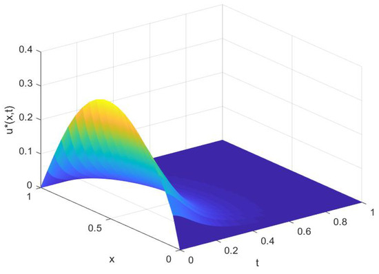
Figure 1. Optimal control $u^{\ast }$.

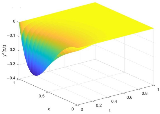
Figure 2. Optimal State $y^{\ast }$.

6. Conclusions

In this paper, we were concerned with the optimal control problem governed by the nonlinear degenerate parabolic equations in multi-dimensional space. Firstly, we proved the existence of the solutions to the optimal control problems governed by the nonlinear degenerate parabolic equations. Secondly, we derived the first-order necessary condition for the linear case and prove the global uniqueness of the optimal control. Thirdly, we derived the first order necessary condition for the nonlinear case and prove the local uniqueness of the optimal control. Finally, we showed a numerical example to rigorously substantiate the validity and applicability of the theoretical outcomes presented herein. Our work provides a research approach for the optimal control problem of degenerate parabolic equations. In the future, there are many topics we will consider regarding the optimal control problems of degenerate parabolic equations, such as the optimal control problem of degenerate parabolic equations with convection terms, the optimal control problem of coupled degenerate parabolic equations, and the optimal boundary control problem of degenerate parabolic equations.

References

- Baranovskii, E.S. Feedback optimal control problem for a network model of viscous fluid flows. Math. Notes 2022, 112, 26–39. [Google Scholar] [CrossRef]
- Baranovskii, E.S. Optimal control for steady flows of the Jeffreys fluids with slip boundary condition. J. Appl. Ind. Math. 2014, 8, 168–176. [Google Scholar] [CrossRef]
- Hu, W.; Lai, M.J.; Lee, J. Optimal control for suppression of singularity in chemotaxis via flow advection. Appl. Math. Optim. 2024, 89, 57. [Google Scholar] [CrossRef]
- Casas, E.; Kunisch, K. Infinite horizon optimal control problems for a class of semilinear parabolic equations. SIAM J. Control Optim. 2022, 60, 2070–2094. [Google Scholar] [CrossRef]
- Casas, E.; Yong, J. Optimal control of a parabolic equation with memory. ESAIM COCV 2023, 29, 23. [Google Scholar] [CrossRef]
- Tröltzsch, F. Optimal Control of Partial Differential Equations: Theory, Methods, and Applications; American Mathematical Society: Providence, RI, USA, 2010; Volume 112. [Google Scholar]
- Lions, J.L. Optimal Control of Systems Governed by Partial Differential Equations; Springer: Berlin/Heidelberg, Germany, 1971. [Google Scholar]
- Cannarsa, P.; Martinez, P.; Vancostenoble, J. Null controllability of degenerate heat equations. Adv. Differ. Equ. 2005, 10, 153–190. [Google Scholar] [CrossRef]
- Jiang, L.S.; Tao, Y.S. Identifying the volatility of underlying assets from option prices. Inverse Problems 2001, 17, 137–155. [Google Scholar]
- North, G.R.; Howard, D.; Pollard, D.; Wielicki, B. Variational formulation of Budyko-Sellers climate models. J. Atmos. Sci. 1979, 36, 255–259. [Google Scholar] [CrossRef][Green Version]
- Deng, Z.; Yang, L. An inverse problem of identifying the radiative coefficient in a degenerate parabolic equation. Chin. Ann. Math. Ser. B 2014, 35, 355–382. [Google Scholar] [CrossRef]
- Lenhart, S.M.; Yong, J. Optimal control for degenerate parabolic equations with logistic growth. Nonlinear Anal. 1995, 25, 681–698. [Google Scholar] [CrossRef]
- Marinoschi, G.; Mininni, R.M.; Romanelli, S. An optimal control problem in coefficients for a strongly degenerate parabolic equation with interior degeneracy. J. Optim. Theory Appl. 2017, 173, 56–77. [Google Scholar] [CrossRef]
- Cannarsa, P.; Martinez, P.; Vancostenoble, J. Carleman estimates for a class of degenerate parabolic operators. SIAM J. Control Optim. 2008, 47, 1–19. [Google Scholar] [CrossRef]
- Du, R. Null controllability for a class of degenerate parabolic equations with the gradient terms. J. Evol. Equ. 2019, 19, 585–613. [Google Scholar] [CrossRef]
- Wang, C. Approximate controllability of a class of semilinear systems with boundary degeneracy. J. Evol. Equ. 2010, 10, 163–193. [Google Scholar] [CrossRef]
- Wang, C.; Du, R. Approximate controllability of a class of semilinear degenerate systems with convection term. J. Differ. Equ. 2013, 254, 3665–3689. [Google Scholar] [CrossRef]
- Wang, C.; Du, R. Carleman estimates and null controllability for a class of degenerate parabolic equations with convection terms. SIAM J. Control Optim. 2014, 52, 1457–1480. [Google Scholar] [CrossRef]
- Yin, J.; Wang, C. Evolutionary weighted p-Laplacian with boundary degeneracy. J. Differ. Equ. 2007, 237, 421–445. [Google Scholar] [CrossRef]
- Casas, E.; Fernández, L.A. Distributed Control of Systems Governed by a General Class of Quasinlinear Elliptic Equations. J. Differ. Equ. 1993, 104, 20–47. [Google Scholar] [CrossRef]
- Stojanovic, S. Optimal damping control and nonlinear elliptic systems. SIAM J. Control Optim. 1991, 29, 594–608. [Google Scholar] [CrossRef]
Disclaimer/Publisher’s Note: The statements, opinions and data contained in all publications are solely those of the individual author(s) and contributor(s) and not of MDPI and/or the editor(s). MDPI and/or the editor(s) disclaim responsibility for any injury to people or property resulting from any ideas, methods, instructions or products referred to in the content. |
© 2024 by the authors. Licensee MDPI, Basel, Switzerland. This article is an open access article distributed under the terms and conditions of the Creative Commons Attribution (CC BY) license (https://creativecommons.org/licenses/by/4.0/).