Abstract
The history of variational calculus dates back to the late 17th century when Johann Bernoulli presented his famous problem concerning the brachistochrone curve. Since then, variational calculus has developed intensively as many problems in physics and engineering are described by equations from this branch of mathematical analysis. This paper presents two non-classical, distinct methods for solving such problems. The first method is based on the differential transform method (DTM), which seeks an analytical solution in the form of a certain functional series. The second method, on the other hand, is based on the physics-informed neural network (PINN), where artificial intelligence in the form of a neural network is used to solve the differential equation. In addition to describing both methods, this paper also presents numerical examples along with a comparison of the obtained results.Comparingthe two methods, DTM produced marginally more accurate results than PINNs. While PINNs exhibited slightly higher errors, their performance remained commendable. The key strengths of neural networks are their adaptability and ease of implementation. Both approaches discussed in the article are effective for addressing the examined problems.
Keywords:
variational calculus; ordinary differential equation; differential transform method; physics-informed neural network MSC:
65L05
1. Introduction
The issues in the calculus of variations have rich applications in many different problems [1]. Using these methods, one can, for example, search for curves connecting fixed points (also considering problems with a moving boundary) and satisfying certain conditions (such as minimal length or the shortest time to travel between them), surfaces meeting specific conditions (such as the surface with the smallest area connecting two fixed circles), problems concerning the propagation of light in inhomogeneous media, isoperimetric problems, geodesic curves, quantum mechanics, hydrodynamics, and many others [2,3,4,5].
The problem of variational calculus can be described in many different ways; this paper focuses on finding the extremum of the following functional:
where is the sought-after n-times differentiable function defined in the interval , which satisfies the following boundary conditions:
where , , , , and F is a certain function of variables’ -times differential, defined in the set .
For such a formulated problem, a necessary condition for the functional (1) to attain a local extremum for the sought-after function under the boundary conditions (2) is that the function F satisfies the following differential equation:
(this is the so-called Euler–Poisson equation) with the conditions (2) [6,7].
In the general case, the condition (3) is only a necessary condition for the existence of an extremum of the functional (1). However, in most technical problems, it is also a sufficient condition. Therefore, in this paper, we search for these extrema in this manner.
Equation (3) is a differential equation of the order and appears relatively rarely for larger values of n. It is more commonly encountered for or . In these cases, it takes the following form:
In the special case of , this equation is known as the Euler equation. Often, there are problems where the function F depends on many unknown functions, e.g., (and their derivatives). In such cases, the necessary condition for the existence of an extremum of the functional (the Euler–Lagrange equations) reduces to a system of differential equations.
Unfortunately, very often, the differential equations (or their systems) obtained from the corresponding conditions are nonlinear or cannot be expressed in normal form (which is required by many methods for solving such problems, including classical ones like the Runge–Kutta method and less-known ones like the Adomian decomposition method [8,9]). For this reason, we need to seek new methods that can handle such forms of the problem.
Such methods include the differential transformation method (DTM) discussed in Section 2 and the physics-informed neural networks (PIINs) presented in Section 3. PINNs are a type of specifically designed neural network devoted to solving problems involving differential equations that describe physical laws. PINNs integrate knowledge of physical laws, allowing for the more accurate and efficient modeling of physical phenomena compared with traditional neural networks. PINNs can generalize better to unseen conditions because they are guided by underlying physical laws, which remain consistent across different scenarios. This contrasts traditional neural networks that might struggle to extrapolate beyond their training data. Section 4 is devoted to numerical examples illustrating the effectiveness of both methods and comparing them using selected examples.
2. DTM Method
The differential transform method (DTM) was proposed at the end of the 20th century and was quickly recognized and adapted to solve many different problems. Initially, it was used to solve ordinary differential equations, but its applications have expanded to the systems of such equations [10,11,12,13,14,15], partial differential equations [16,17], differential algebraic equations [18], integral equations [19,20], delay differential equations [21,22], fuzzy differential equations [23,24], and fractional differential equations [25,26,27,28]. This method has also been applied to certain important types of equations, such as Schrödinger equations and nonlinear Klein–Gordon equations, and in modeling predator–prey phenomena [29,30,31], among many other applications [32,33,34,35,36].
If a function, f, can be expanded into a Maclaurin series (such a function is called the original), then for this function, we can write the following:
Thus, knowing the properties of such a transformation and the transforms of basic functions, we can solve many of the problems mentioned in the previous paragraph.
Below, we present the transforms of selected functions and selected properties of DTM (the included functions and properties were used in the examples presented in Section 4; proofs of these properties, among others, can be found in [16,25]).
Theorem 1.
Let x be an element of the domain of the considered function, f, and .
If , , then
If , , then
If , , then
If , , then
If , then
If , , then
If , then
If , then
If , then
If , then
3. Physics-Informed Neural Network
Physics-informed neural networks (PINNs) represent a novel approach to solving differential equations (both ordinary and partial) and differential-integral equations, harnessing the power of deep learning. Among the pioneering works on this approach are the papers by Raisi et al. [37] and Karniadakis et al. [38]. PINNs integrate the principles of physics in the form of differential equations with a neural network architecture. This methodology embeds differential equations and initial/boundary conditions into the loss function of the neural network, ensuring that predictions align with the equations describing the system. As a result, PINNs offer a flexible and efficient alternative to traditional numerical methods, which often face limitations related to computational costs and scalability, especially in high-dimensional spaces. Once the model is trained, it can provide solutions for any grid, making this approach advantageous over classical methods like finite difference schemes. Additionally, PINNs excel in handling complex boundary and initial conditions, and they can directly incorporate experimental data into the model. This capability not only enhances solution accuracy but also enables the model to learn and adapt to real-world scenarios where data may be sparse or noisy. Consequently, PINNs have achieved significant success in various applications, including fluid dynamics, materials science, and biological systems [39,40,41].
A PINN architecture consists of classical components of the feedforward and backpropagation of neural networks: hidden layers, nodes per hidden layer, and activation functions. To train a neural network, an optimization method like the adam optimizer is used. The PINN system presented in the article consists of two main modules (see Figure 1): a fully connected neural network and a loss function module that computes the loss as the weighted norm of both the governing ODE equation and boundary condition’s residuals.
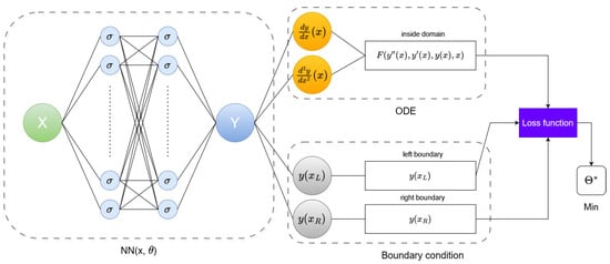
Figure 1.
Diagram of physics-informed neural network for ODE with Dirichlet boundary conditions.
For the considered ordinary differential equation, the following applies:
With Dirichlet boundary conditions, the following apply:
The loss function takes the following form:
where N is the number of collocation/training points inside domain . After building the neural network and defining the loss function, the neural network is then trained to find the best parameters, (weights and biases), by minimizing the loss function, .
4. Numerical Examples
4.1. Example 1
Let us consider a functional,
with boundary conditions,
In this case,
and therefore, according to (3), for ,
which, after some transformation, gives the following equation:
Taking into account the conditions (16), we therefore have to solve an ordinary second-order differential equation (a linear, non-homogeneous one with constant coefficients), where the exact solution to this equation is the following function:
4.1.1. DTM—Example 1
Applying the DTM to Equation (17) (utilizing properties (4), (8), (9), (13)), for , we obtain the following:
whereby from the condition , we know that . Assuming in (18), we obtain the following:
Notice that neither for nor for are we able to determine the value of —this is because the second condition (16) takes the form (the desired form would be . Therefore, let us assume . Taking , we sequentially obtain the following:
In the general case, we can note that and ; for , we have and for even numbers, i, and and for odd numbers, j.
Therefore, we can represent the sought-after function, y, as follows:
which, after using a known Taylor series, takes the following form:
There is still an unknown value of s to find. Using the second condition (16), i.e., , we obtain the following:
This result allows for the final form of the following solution,
which fully coincides with the exact solution. Of course, this is not the standard case—in most instances, we can only find an approximate solution, as we present in the subsequent examples.
4.1.2. PINNs—Example 1
Now, we solve Equation (17) using neural networks. In this case, a fully connected neural network of a depth of 4 with 3 hidden layers and 10 neurons per layer is used. As an optimizer, the Adam method is used with a learning rate of . The hyperbolic tangent is assumed as the activation function. Figure 2 shows the obtained approximate solution (left plot, black dots) along with the errors of this approximation (right plot). The obtained solution fits the exact solution quite well. The maximum error is approximately .
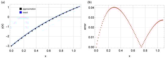
Figure 2.
The exact solution, (solid blue line); the approximate solution (black dots)—Figure (a); and the errors of the approximate solution—Figure (b), example 1.
4.2. Example 2
Consider following functional,
with conditions
In this case, we have
and therefore we, can, according to (3) for , write
which, after some transformation, leads to the equation
with conditions (20) (other solutions, and , are neglected because they do not meet the conditions (20)).
4.2.1. DTM—Example 2
Applying the DTM of transformation to Equation (21) (here, we use the properties (8), (9), (12), and (13)), for , we obtain
and according to the condition, implies that .
Similarly to before, taking successive values, , in (22), we are not be able to find the value of . Therefore, assume ; as a result, , , and
This time, we are not able to find a function defined by the Taylor series of the obtained terms. Therefore, we must limit ourselves to finding an approximate solution, , of the form
which depends on the unknown value of parameter s. The value of this parameter can be found using the second of the conditions (20), i.e., . Proceeding in this way and taking , an approximate solution, , of the following form is obtained:
Solving the equation , we unfortunately obtain three real solutions: , , and . Therefore, it is necessary to choose the appropriate one. To achieve this, we examine the error as follows:
In this case, it turns out that the best value is . For this value, we obtain an approximate solution:
Following a similar approach but taking (again choosing the best value of s), we obtain the following solution:
In Figure 3, we present the exact solution, , the approximate solutions, and , and the errors, , of these solutions, where
and the exact solution has the following form:
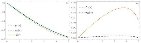
Figure 3.
Exact solution, (solid green line); approximate solution, (dashed orange line); approximate solution, (dashed blue line)—Figure (a)—and errors, , of these approximations—Figure (b), example 2.
4.2.2. PINNs—Example 2
The same Equation (21) was also solved using a physics-informed neural network. In this example, a fully connected neural network of a depth of 4 with 3 hidden layers and 10 neurons per layer was used. The Adam optimizer with a learning rate of was employed and the hyperbolic tangent is assumed as the activation function. Inside the domain, 128 training points were considered. Figure 4 depicts the obtained approximate solution (left plot, black dots) along with the errors of this approximation (right plot). The obtained solution is very close to the exact solution. The maximum error does not exceed .
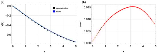
Figure 4.
The exact solution (solid blue line), the approximate solution (black dots)—Figure (a)—and the errors of the approximate solution—Figure (b), example 2.
4.3. Example 3
In the third example, the following equation is considered,
which is supplemented by the following conditions:
In this case,
and therefore, according to (3), for , we obtain the following,
which brings us to the follwing equation,
with conditions (24).
4.3.1. DTM—Example 3
Applying the DTM of transformation to Equation (25) (we use the properties (5)–(9), (11), and (13)), the following equation is obtained for :
Given successive values of in (26), it is impossible to find the values , , and , so we assume , , and , , . Therefore i , , , and
Again, we are unable to find a function with a Taylor series defined by these terms based on the form of the found terms. We must therefore limit ourselves to finding an approximate solution of the form ,
which additionally depends on an unknown parameter, , . These parameters are determined using conditions (24) (this time we have a unique set of exactly four constants ). Proceeding in this way and taking , we obtain an approximate solution of the form :
Proceeding similarly, but taking (again the conditions (24) imply a unique solution to the parameters , and ), we obtain the following solution:
Figure 5 shows the exact solution , the approximate solutions, and , and the errors, , of these solutions. In following formula of error,
denotes the exact solution obtained form Wolfram Mathematica 14.0 [42,43]. As can be seen in Figure 5, the difference in errors between solutions and is significant. The maximum error for does not exceed , whereas for the solution , this error is approximately .
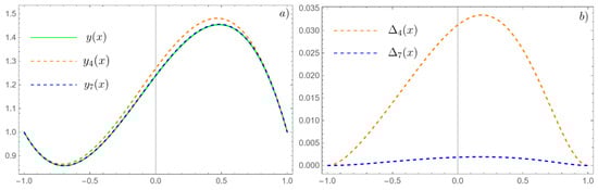
Figure 5.
Exact solution, (solid green line); approximate solution, (dashed orange line); approximate solution, (dashed blue line)—Figure (a)—and errors of these approximations—Figure (b), example 3.
4.3.2. PINNs—Example 3
Similar to previous examples, the following network architecture is assumed: 3 hidden layers with 10 neurons per layer. Inside the domain, 128 training points are used. The hyperbolic tangent is assumed as the activation function. The solution obtained after training the model is depicted in Figure 6. The solution using PINNs fits the exact solution quite well, with errors not exceeding .
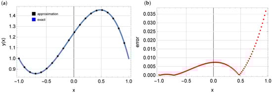
Figure 6.
The exact solution (solid blue line); the approximate solution (black dots)—Figure (a)—and the errors of the approximate solution—Figure (b), example 3.
4.4. Comparison of DTM and PINNs Results
In this section, errors obtained from the two methods are compared for examples 2 and 3. In the case of example 1, the DTM method provides the exact solution. Figure 7 presents error plots obtained from both methods, specifically for example 2 (Figure 7a) and example 3 (Figure 7b). As observed in Figure 7, the smallest errors were obtained for DTM with (for example 2) and (for example 3). The errors of the solutions obtained using neural networks are slightly larger but still smaller than those from DTM with (for example 2) and (for example 3). Both methods produced solutions of good quality.
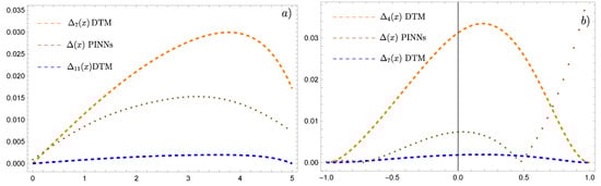
Figure 7.
Comparison of absolute errors of the DTM and PINNs for example 2—figure (a) and for example 3—figure (b).
5. Conclusions
The paper presents two different methods for solving variational calculus problems involving differential equations.
The first method, the DTM, is characterized by its flexibility in both the form of the differential equation and the boundary conditions. One of its strengths is its scalability to handle approximate solutions of varying orders, and sometimes it even allows for a prediction of the exact solution based on the form of the coefficients found for . However, there are some drawbacks to this method. One notable challenge is the difficulty in automating the process of solving a given problem. It is complex to develop a program that can generate an approximate solution solely based on the form of the differential equation and the boundary conditions. It is often easier to manually construct a discrete counterpart of the differential equation, develop a methodology for finding the unknown coefficients, , and then utilize appropriate software tools for further refinement.
The second presented approach—PINNs (physics-informed neural networks)—utilizes neural networks to solve the relevant differential equation. One advantage of this method is its relatively straightforward implementation and flexibility. Once the model for the differential equation is trained, it can provide solutions for different grids (input points) without recalculating the problem each time.
Comparing both methods, it can be observed that slightly more accurate results were obtained using the DTM. The results from PINNs includes slightly larger errors compared with those obtained using the DTM, but they are still of good quality. The advantage of neural networks lies in their flexibility and relatively straightforward implementation. Both methods presented in the article are suitable for solving the considered issues.
In the future, the authors plan to apply PINNs to solve direct and inverse problems in partial differential equations involving fractional-order derivatives.
Author Contributions
Conceptualization, R.B. and M.P.; methodology, R.B. and M.P.; software, R.B. and M.P.; validation, R.B. and M.P.; formal analysis, R.B. and M.P.; investigation, R.B. and M.P.; writing—original draft preparation, R.B. and M.P.; writing—review and editing, R.B. and M.P.; visualization, R.B. and M.P.; supervision, R.B. and M.P. All authors have read and agreed to the published version of the manuscript.
Funding
This research received no external funding.
Institutional Review Board Statement
Not applicable.
Informed Consent Statement
Not applicable.
Data Availability Statement
The data presented in this study are available on request from the corresponding author.
Conflicts of Interest
The author declare no conflict of interest.
References
- Struwe, M. Variational Methods; Springer: New York, NY, USA, 2000; pp. 32–58. [Google Scholar]
- Borghi, R. The variational method in quantum mechanics: An elementary introduction. Eur. J. Phys. 2018, 39, 035410. [Google Scholar] [CrossRef]
- Esteban, M.; Lewin, M.; Séré, E. Variational methods in relativistic quantum mechanics. Bull. Am. Math. Soc. 2008, 45, 535–593. [Google Scholar] [CrossRef]
- Mihlin, S.G. Variational Methods of Solving Linear and Nonlinear Boundary Value Problems. Differential Equations and Their Applications; Publishing House of the Czechoslovak Academy of Sciences: Prague, Czech Republic, 1963; pp. 77–92. Available online: http://eudml.org/doc/220899 (accessed on 7 July 2024).
- Sysoev, D.V.; Sysoeva, A.A.; Sazonova, S.A.; Zvyagintseva, A.V.; Mozgovoj, N.V. Variational methods in relativistic quantum mechanics. In IOP Conference Series: Materials Science and Engineering; IOP Publishing: Bristol, UK, 2021; Volume 1047, p. 012195. [Google Scholar]
- Courant, R.; Hilbert, D. Methods of Mathematical Physics; Wiley-VCH: New York, NY, USA, 1962; Volume I. [Google Scholar]
- Fox, C. An Introduction to the Calculus of Variations; Courier Corporation: North Chelmsford, MA, USA, 1987. [Google Scholar]
- Grzymkowski, R.; Pleszczynski, M.; Słota, D. Comparing the Adomian decomposition method and the Runge–Kutta method for solutions of the Stefan problem. Int. J. Comput. Math. 2006, 83, 409–417. [Google Scholar] [CrossRef]
- Grzymkowski, R.; Pleszczynski, M.; Słota, D. The two-phase Stefan problem solved by the Adomian decomposition method. In Proceedings of the 15th IASTED International Conference Applied Simulation and Modelling, Rhodos, Greece, 26–28 June 2006; pp. 511–516. [Google Scholar]
- Zhou, J.K. Differential Transformation and Its Applications for Electrical Circuits; Huazhong University Press: Wuhan, China, 1986. [Google Scholar]
- Ayaz, F. Solutions of the system of differential equations by differential transform method. Appl. Math. Comput. 2004, 147, 547–567. [Google Scholar] [CrossRef]
- Grzymkowski, R.; Pleszczynski, M. Application of the Taylor transformation to the systems of ordinary differential equations. In Information and Software Technologies, Proceedings of the 24th International Conference, ICIST 2018, Vilnius, Lithuania, 4–6 October 2018; Springer International Publishing: Berlin/Heidelberg, Germany, 2018; Volume 24, pp. 379–387. [Google Scholar]
- Hetmaniok, E.; Pleszczyński, M. Comparison of the selected methods used for solving the ordinary differential equations and their systems. Mathematics 2022, 10, 306. [Google Scholar] [CrossRef]
- Keskin, Y.; Oturanc, G. Reduced differential transform method for partial differential equations. Int. J. Nonlinear Sci. Numer. Simul. 2009, 10, 741–750. [Google Scholar] [CrossRef]
- Mirzaee, F. Differential transform method for solving linear and nonlinear systems of ordinary differential equations. Appl. Math. Sci. 2011, 5, 3465–3472. [Google Scholar]
- Ayaz, F. On the two-dimensional differential transform method. Appl. Math. Comput. 2003, 143, 361–374. [Google Scholar] [CrossRef]
- Kanth, A.R.; Aruna, K. Differential transform method for solving linear and non-linear systems of partial differential equations. Phys. Lett. A 2008, 372, 6896–6898. [Google Scholar] [CrossRef]
- Ayaz, F. Applications of differential transform method to differential-algebraic equations. Appl. Math. Comput. 2004, 152, 649–657. [Google Scholar] [CrossRef]
- Biazar, J.; Eslami, M.; Islam, M.R. Differential transform method for special systems of integral equations. J. King Saud Univ.-Sci. 2012, 24, 211–214. [Google Scholar] [CrossRef]
- Celik, E.; Tabatabaei, K. Solving a Class of Volterra Integral Equation Systems by the Differential Transform Method. Int. J. Nonlinear Sci. Numer. Simul. 2013, 16, 87–91. [Google Scholar]
- Liu, B.; Zhou, X.; Du, Q. Differential transform method for some delay differential equations. Appl. Math. 2015, 6, 585. [Google Scholar] [CrossRef]
- Hetmaniok, E.; Pleszczyński, M.; Khan, Y. Solving the Integral Differential Equations with Delayed Argument by Using the DTM Method. Sensors 2022, 22, 4124. [Google Scholar] [CrossRef] [PubMed]
- Allahviranloo, T.; Kiani, N.A.; Motamedi, N. Solving fuzzy differential equations by differential transformation method. Inf. Sci. 2009, 179, 956–966. [Google Scholar] [CrossRef]
- Osman, M.; Almahi, A.; Omer, O.A.; Mustafa, A.M.; Altaie, S.A. Approximation Solution for Fuzzy Fractional-Order Partial Differential Equations. Fractal Fract. 2022, 6, 646. [Google Scholar] [CrossRef]
- Arikoglu, A.; Ozkol, I. Solution of fractional differential equations by using differential transform method. Chaos Solitons Fractals 2007, 34, 1473–1481. [Google Scholar] [CrossRef]
- Neelma; Eiman; Shah, K. Analytical and Qualitative Study of Some Families of FODEs via Differential Transform Method. Foundations 2022, 2, 6–19. [Google Scholar] [CrossRef]
- Odibat, Z.; Momani, S.; Erturk, V.S. Generalized differential transform method: Application to differential equations of fractional order. Appl. Math. Comput. 2008, 197, 467–477. [Google Scholar] [CrossRef]
- Rysak, A.; Gregorczyk, M. Differential Transform Method as an Effective Tool for Investigating Fractional Dynamical Systems. Appl. Sci. 2021, 11, 6955. [Google Scholar] [CrossRef]
- Kanth, A.R.; Aruna, K. Differential transform method for solving the linear and nonlinear Klein–Gordon equation. Comput. Phys. Commun. 2009, 180, 708–711. [Google Scholar] [CrossRef]
- Kanth, A.R.; Aruna, K. Two-dimensional differential transform method for solving linear and non-linear Schrödinger equations. Chaos Solitons Fractals 2009, 41, 2277–2281. [Google Scholar] [CrossRef]
- Tari, A. The Differential Transform Method for solving the model describing biological species living together. Iran. J. Math. Sci. Inform. 2012, 7, 63–74. [Google Scholar]
- Gupta, R.; Selvam, J.; Vajravelu, A.; Nagapan, S. Analysis of a Squeezing Flow of a Casson Nanofluid between Two Parallel Disks in the Presence of a Variable Magnetic Field. Symmetry 2023, 15, 120. [Google Scholar] [CrossRef]
- Kumar, R.S.V.; Sarris, I.E.; Sowmya, G.; Abdulrahman, A. Iterative Solutions for the Nonlinear Heat Transfer Equation of a Convective-Radiative Annular Fin with Power Law Temperature-Dependent Thermal Properties. Symmetry 2023, 15, 1204. [Google Scholar] [CrossRef]
- Zhang, L.; Han, M.; Zhang, Q.; Hao, S.; Zhen, J. Analysis of Dynamic Characteristics of Attached High Rise Risers. Appl. Sci. 2023, 13, 8767. [Google Scholar] [CrossRef]
- Demir, Ö. Differential Transform Method for Axisymmetric Vibration Analysis of Circular Sandwich Plates with Viscoelastic Core. Symmetry 2022, 14, 852. [Google Scholar] [CrossRef]
- Brociek, R.; Pleszczyński, M. Comparison of Selected Numerical Methods for Solving Integro-Differential Equations with the Cauchy Kernel. Symmetry 2024, 16, 233. [Google Scholar] [CrossRef]
- Raissi, M.; Perdikaris, P.; Karniadakis, G.E. Physics-informed neural networks: A deep learning framework for solving forward and inverse problems involving nonlinear partial differential equations. J. Comput. Phys. 2019, 378, 686–707. [Google Scholar] [CrossRef]
- Karniadakis, G.E.; Kevrekidis, I.G.; Lu, L.; Perdikaris, P.; Wang, S.; Yang, L. Physics-informed machine learning. Nat. Rev. Phys. 2021, 3, 422–440. [Google Scholar] [CrossRef]
- Eivazi, H.; Wang, Y.; Vinuesa, R. Physics-informed deep-learning applications to experimental fluid mechanics. Meas. Sci. Technol. 2024, 35, 075303. [Google Scholar] [CrossRef]
- Cuomo, S.; Schiano Di Cola, V.; Giampaolo, F.; Rozza, G.; Raissi, M.; Piccialli, F. Scientific Machine Learning Through Physics–Informed Neural Networks: Where we are and What’s Next. J. Sci. Comput. 2022, 92, 88. [Google Scholar] [CrossRef]
- Ahmadi Daryakenari, N.; De Florio, M.; Shukla, K.; Karniadakis, G.E. AI-Aristotle: A physics-informed framework for systems biology gray-box identification. PLoS Comput. Biol. 2024, 20, 1–33. [Google Scholar] [CrossRef] [PubMed]
- Hastings, C.; Mischo, K.; Morrison, M. Hands-on Start to Wolfram Mathematica and Programming with the Wolfram Language, 3rd ed.; Wolfram Media, Inc.: Champaign, IL, USA, 2020. [Google Scholar]
- Wolfram, S. The Mathematica Book, 5th ed.; Wolfram Media, Inc.: Champaign, IL, USA, 2003. [Google Scholar]


Disclaimer/Publisher’s Note: The statements, opinions and data contained in all publications are solely those of the individual author(s) and contributor(s) and not of MDPI and/or the editor(s). MDPI and/or the editor(s) disclaim responsibility for any injury to people or property resulting from any ideas, methods, instructions or products referred to in the content. |
© 2024 by the authors. Licensee MDPI, Basel, Switzerland. This article is an open access article distributed under the terms and conditions of the Creative Commons Attribution (CC BY) license (https://creativecommons.org/licenses/by/4.0/).