On Some Results of the Nonuniqueness of Solutions Obtained by the Feynman–Kac Formula

Abstract

The Feynman–Kac formula establishes a link between parabolic partial differential equations and stochastic processes in the context of the Schrödinger equation in quantum mechanics. Specifically, the formula provides a solution to the partial differential equation, expressed as an expectation value for Brownian motion. This paper demonstrates that the Feynman–Kac formula does not produce a unique solution but instead carries infinitely many solutions to the corresponding partial differential equation.

1. Introduction

In the 1940s, Feynman [1] disclosed that the Schrödinger equation, which governs the time evolution of quantum states in quantum mechanics, could be solved by averaging over sample paths, an observation which led him to a far-reaching reformulation of the quantum theory in terms of path integrals [2,3]. Based on this idea, Kac recognized that a similar representation could be given for solutions of the heat transfer equation [4,5]. Accordingly, this representation is now referred to as the Feynman–Kac formula, which verifies and extends Feynman’s path integrals [6]. The Feynman–Kac formula has numerous applications in various fields including mathematics, statistics, physics, chemistry, and finance [7,8], providing an intriguing connection between solutions of elliptic and parabolic differential equations and stochastic processes. Specifically, it provides a method for solving a variety of partial differential equations (PDEs) through random path simulations of a stochastic process. For instance, in quantitative finance, the relationship between geometric Brownian motion and the Black–Scholes PDE is a special case of the Feynman–Kac theorem [9]. Conversely, some stochastic differential equations describing random processes can be examined by deterministic methods [10].

To present the Feynman–Kac formula, we consider the continuous functions $f:{\mathbb{R}}^d\to \mathbb{R}$, $k:{\mathbb{R}}^d\to {\mathbb{R}}_{\ge 0}$, and $g:{\mathbb{R}}^d\times [0,T]\to \mathbb{R}$, where $T>0$ is fixed. Suppose that v is a continuous, real-valued function of class $C^{2,1}$ on ${\mathbb{R}}^d\times [0,T]$ and satisfies

$$\begin{array}{c}\hfill -\frac{\partial v}{\partial t}+kv=\frac{1}{2}\sum _{i=1}^d\frac{{\partial }^{2}v}{\partial x_i^2}+g\end{array}$$

(1)

with the terminal condition $(\mathit{x}\in {\mathbb{R}}^d)$

$$\begin{array}{c}\hfill v(\mathit{x},T)=f\left(\mathit{x}\right).\end{array}$$

(2)

Then, the function v is said to be a solution of the Cauchy problem for the backward heat Equation (1) with potential k and Lagrangian g, subject to the terminal condition in Equation (2). Note also that Equation (1) with $g=0$ corresponds precisely to the Schrödinger equation (in the imaginary time) for a particle in potential k. Suppose that

$$\underset{0\le t\le T}{max}\left|v(\mathit{x},t)\right|+\underset{0\le t\le T}{max}\left|g(\mathit{x},t)\right|\le K{e}^{{a\parallel \mathit{x}\parallel }^2}\mathrm{for}\forall \mathit{x}\in {\mathbb{R}}^d,$$

(3)

where K is a positive constant and $0<a<Td/2$. The Feynman–Kac formula consists of the existence part and the uniqueness part as follows: The former states that v admits the stochastic representation

$$\begin{array}{cc}\hfill v(\mathit{x},t)=& E_T^{\mathit{x}}\left\{f\left({\mathit{W}}_{T-t}\right)exp\left[-{\int }_0^{T-t}k\left({\mathit{W}}_s\right)ds\right]\right.\hfill \\ \hfill & \left.+{\int }_0^{T-t}g\left({\mathit{W}}_{\theta },t+\theta \right)exp\left[-{\int }_0^{\theta }k\left({\mathit{W}}_s\right)ds\right]d\theta \right\}\hfill \end{array}$$

(4)

for any $t\in [0,T]$ and $\mathit{x}\in {\mathbb{R}}^d$, where $\left\{{\mathit{W}}_t\right\}$ is a d-dimensional Brownian motion and $E_T^{\mathit{x}}(·)$ is the expectation operator with ${\mathit{W}}_T=\mathit{x}$. Then, the latter asserts that such a solution is unique, as remarked in Refs. [11] (p. 268) and [12] (p. 120). Readers may also refer to Refs. [6] (Chapter 3), [13] (Section 11.4), and [14] (Section 8.2), for further details on the Feynman–Kac formula.

In this paper, we present a counterexample that violates the uniqueness of the Feynman–Kac formula. Specifically, it is disclosed that the Feynman–Kac formula carries infinitely many solutions rather than a unique solution. The possibility of nonuniqueness alerts us that the solution method based on the Feynman–Kac formula may lead to extraneous and irrelevant results. These implications are discussed in relation to the initial conditions.

2. A Boundary-Value Problem and Its Feynman–Kac Solution

We consider a simple example for $d=1$ with

$$\begin{array}{c}\hfill k\left(x\right)\equiv 0,g(x,t)\equiv 0,f\left(x\right)=exp(-|x\left|\right)\end{array}$$

(5)

and let $u(x,\tau )\equiv v(x,t)$ with $\tau \equiv T-t$. General cases with nonvanishing k and g are considered later in Section 3. Then, Equations (1) and (2) become, respectively,

$$\begin{array}{cc}\hfill & \frac{\partial u}{\partial \tau }=\frac{1}{2}\frac{{\partial }^{2}u}{\partial x^2}\mathrm{on}\mathbb{R}\times [0,T],\hfill \end{array}$$

(6)

$$\begin{array}{cc}\hfill & u(x,0)=exp\left(-\left|x\right|\right)\mathrm{for}x\in \mathbb{R}.\hfill \end{array}$$

(7)

It is well known (see, e.g., [15]) that $\frac{1}{\sqrt{\tau }}\varphi \left(\frac{x}{\sqrt{\tau }}\right)$ is the fundamental solution of the PDE (6), where $\varphi \left(z\right)\equiv \frac{1}{\sqrt{2\pi }}exp\left(-\frac{1}{2}{z}^2\right)$ is the probability density function of the standard Gaussian random variable.

We now define the function

$$\begin{array}{cc}\hfill g_0(x,\tau )& \equiv E_0^x\left(u\left(W_{\tau },0\right)\right)={\int }_{-\infty }^{\infty }exp\left(-\left|w\right|\right)\frac{1}{\sqrt{\tau }}\varphi \left(\frac{w-x}{\sqrt{\tau }}\right)dw\hfill \end{array}$$

(8)

for $\tau >0$, which, according to the Feynman–Kac formula, satisfies the heat transfer PDE (6) and the initial condition in Equation (7). Equation (8) is divided into two parts:

$$\begin{array}{c}\hfill g_0(x,\tau )=I_{1,0}(x,\tau )+I_{2,0}(x,\tau )\end{array}$$

(9)

with

$$\begin{array}{cc}\hfill & I_{1,0}(x,\tau )\equiv E_0^x\left(exp\left(-|W_{\tau }|\right){\mathbf{1}}_{[0,\infty )}\left(W_{\tau }\right)\right)=exp\left(-x+\frac{\tau }{2}\right)\mathrm{\Phi }\left(\frac{x-\tau }{\sqrt{\tau }}\right),\hfill \end{array}$$

(10)

$$\begin{array}{cc}\hfill & I_{2,0}(x,\tau )\equiv E_0^x\left(exp\left(-|W_{\tau }|\right){\mathbf{1}}_{(-\infty ,0)}\left(W_{\tau }\right)\right)=exp\left(x+\frac{\tau }{2}\right)\mathrm{\Phi }\left(-\frac{x+\tau }{\sqrt{\tau }}\right),\hfill \end{array}$$

(11)

where ${\mathbf{1}}_A(·)$ is the indicator function of a subset A and $\mathrm{\Phi }\left(z\right)\equiv {\int }_{-\infty }^z\varphi \left(y\right)dy$ is the cumulative distribution function of the standard Gaussian random variable. It is then easy to show that $I_{1,0}(x,\tau )$ and $I_{2,0}(x,\tau )$ satisfy the heat transfer PDE:

$$\begin{array}{c}\hfill \frac{\partial I_{1,0}(x,\tau )}{\partial \tau }=\frac{1}{2}\frac{{\partial }^2{I}_{1,0}(x,\tau )}{\partial x^2}\mathrm{and}\frac{\partial I_{2,0}(x,\tau )}{\partial \tau }=\frac{1}{2}\frac{{\partial }^2{I}_{2,0}(x,\tau )}{\partial x^2}.\end{array}$$

(12)

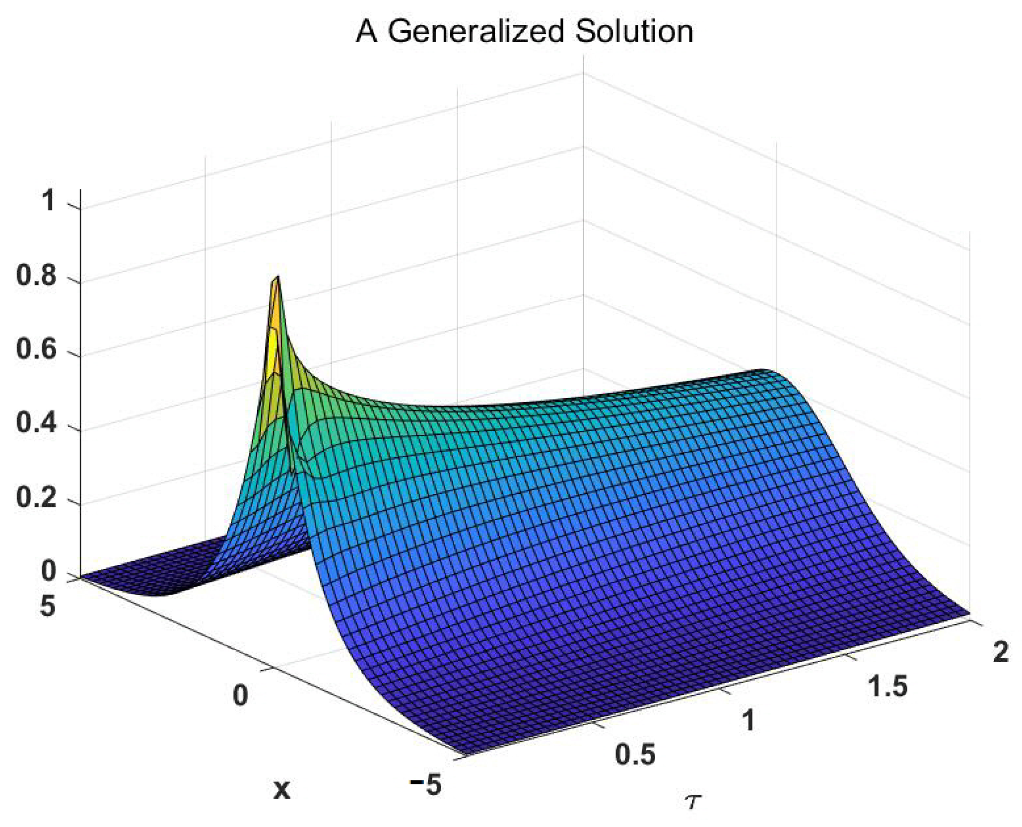
For comparison, we plot the conventional (fundamental) solution in Figure 1 and the generalized solution given by Equation (9) in Figure 2.

Figure 1. Conventional solution ${\tau }^{-1}\varphi (x/\sqrt{\tau })$, called the fundamental solution. The darker the color, the lower the value of the solution.

Figure 2. Generalized solution $g_0(x,\tau )$, given by Equation (9). The darker the color, the lower the value of the solution.

Note that Equation (9) plotted in Figure 2 generalizes the fundamental solution in Figure 1 to a heavy-tailed skew distribution [16].

Here, we remark that $g_0(x,\tau )$ is not defined for $\tau =0$. Accordingly, as in Theorem 55.4 of Körner [17] (p. 277), the initial condition in Equation (7) should be replaced by

$$\begin{array}{c}\hfill \underset{\tau \downarrow 0}{lim}u(x,\tau )=exp(-|x\left|\right)\mathrm{for}x\in \mathbb{R}.\end{array}$$

(13)

This means that the solution $u(x,\tau )$ should be assumed right-continuous at $(x,0)$; otherwise, the heat transfer PDE may not be connected with the initial condition.

3. Kernel Solutions

As discussed in Körner [17] (pp. 338–346), the uniqueness of a heat transfer boundary problem is not as trivial a question as sometimes claimed. The simple uniqueness theorem presented there goes as follows: Let $u(x,\tau ):\mathbb{R}\times {\mathbb{R}}^{+}\to \mathbb{R}$ be twice differentiable satisfying the heat transfer PDE (6). If $u(x,\tau )\to 0$ as $\tau \to 0+$ uniformly for x in any chosen interval $[-X,X]$ and if $u(x,\tau )\to 0$ as $\left|x\right|\to \infty$ uniformly for t in any chosen interval $[0,T]$, then $u(x,\tau )=0$ for all $(x,t)\in \mathbb{R}\times {\mathbb{R}}^{+}.$ However, even the fundamental solution $\frac{1}{\sqrt{\tau }}\varphi \left(\frac{x}{\sqrt{\tau }}\right)$ does not satisfy the former uniformity condition, making this uniqueness theorem not so practical. Recently, on the other hand, general solutions of the heat transfer boundary problem were reported [16,18]. Using those general solutions of the heat transfer boundary problem, we now present additional representations of the Feynman–Kac formula.

For any $m\in {\mathbb{Z}}_{\ge 0}$, we consider the probabilists’ Hermite polynomial of order m:

$$\begin{array}{c}\hfill H{e}_m\left(w\right)\equiv {(-1)}^m{e}^{w^2/2}\frac{d^m}{d{w}^m}{e}^{-w^2/2},\end{array}$$

(14)

the first five of which are given by $H{e}_0\left(w\right)=1$, $H{e}_1\left(w\right)=w$, $H{e}_2\left(w\right)=w^2-1$, $H{e}_3\left(w\right)=w^3-3w$, and $H{e}_4\left(w\right)=w^4-6w^2+3$. For each $m\in {\mathbb{Z}}_{\ge 1}$, we define

$$\begin{array}{cc}\hfill g_m(x,\tau )& \equiv E_0^x\left[u\left(W_{\tau },0\right){\tau }^{-m/2}H{e}_m\left(\frac{W_{\tau }-x}{\sqrt{\tau }}\right)\right],\hfill \end{array}$$

(15)

which can be written as

$$\begin{array}{c}\hfill g_m(x,\tau )=I_{1,m}(x,\tau )+I_{2,m}(x,\tau )\end{array}$$

(16)

with

$$\begin{array}{cc}\hfill & I_{1,m}(x,\tau )\equiv E_0^x\left[u\left(W_{\tau },0\right){\tau }^{-m/2}H{e}_m\left(\frac{W_{\tau }-x}{\sqrt{\tau }}\right){\mathbf{1}}_{[0,\infty )}\left(W_{\tau }\right)\right],\hfill \end{array}$$

(17)

$$\begin{array}{cc}\hfill & I_{2,m}(x,\tau )\equiv E_0^x\left[u\left(W_{\tau },0\right){\tau }^{-m/2}H{e}_m\left(\frac{W_{\tau }-x}{\sqrt{\tau }}\right){\mathbf{1}}_{(-\infty ,0)}\left(W_{\tau }\right)\right].\hfill \end{array}$$

(18)

Here, we note that

$$\begin{array}{cc}\hfill I_{1,m}(x,\tau )& ={\int }_0^{\infty }exp\left(-w\right){\tau }^{-m/2}H{e}_m\left(\frac{w-x}{\sqrt{\tau }}\right){\tau }^{-1/2}\varphi \left(\frac{w-x}{\sqrt{\tau }}\right)dw\hfill \end{array}$$

(19)

and make use of the transform $z=(w-x)/\sqrt{\tau }$ to write

$$\begin{array}{cc}\hfill I_{1,m}(x,\tau )& ={\tau }^{-m/2}exp\left(-x+\frac{\tau }{2}\right){\int }_{-x/\sqrt{\tau }}^{\infty }H{e}_m\left(z\right)\frac{1}{\sqrt{2\pi }}exp\left[-\frac{1}{2}{(z+\sqrt{\tau })}^2\right]dz\hfill \\ \hfill & ={\tau }^{-m/2}exp\left(-x+\frac{\tau }{2}\right){\int }_{-\frac{x-\tau }{\sqrt{\tau }}}^{\infty }H{e}_m\left(u-\sqrt{\tau }\right)\varphi \left(u\right)du\hfill \\ \hfill & ={\tau }^{-m/2}exp\left(-x+\frac{\tau }{2}\right)\sum _{j=0}^m\left(\genfrac{}{}{0pt}{}{m}{j}\right){(-\sqrt{\tau })}^{m-j}{\int }_{-\frac{x-\tau }{\sqrt{\tau }}}^{\infty }H{e}_j\left(u\right)\varphi \left(u\right)du,\hfill \end{array}$$

(20)

where the identity

$$H{e}_l(x+a)=\sum _{j=0}^l\left(\genfrac{}{}{0pt}{}{l}{j}\right)a^{l-j}H{e}_j\left(x\right)$$

(21)

has been used for obtaining the third equality. We further note that

$$H{e}_l\left(x\right)\varphi \left(x\right)=-\frac{d}{dx}{(-1)}^{l-1}\left[\frac{d^{l-1}}{d{x}^{l-1}}\varphi \left(x\right)\right]=-\frac{d}{dx}\left[H{e}_{l-1}\left(x\right)\varphi \left(x\right)\right],$$

(22)

which gives

$$\begin{array}{c}\hfill {\int }_d^{\infty }H{e}_l\left(x\right)\varphi \left(x\right)dx=\left\{\begin{array}{cc}1-\mathrm{\Phi }\left(d\right)=\mathrm{\Phi }(-d)\hfill & \mathrm{for}l=0,\hfill \\ H{e}_{l-1}\left(d\right)\varphi \left(d\right)\hfill & \mathrm{for}l=1,2,\dots \hfill \end{array}\right.\end{array}$$

(23)

and

$$\begin{array}{c}\hfill {\int }_{-\infty }^{d}H{e}_l\left(x\right)\varphi \left(x\right)dx=\left\{\begin{array}{cc}\mathrm{\Phi }\left(d\right)\hfill & \mathrm{for}l=0,\hfill \\ -H{e}_{l-1}\left(d\right)\varphi \left(d\right)\hfill & \mathrm{for}l=1,2,\dots .\hfill \end{array}\right.\end{array}$$

(24)

Putting Equation (23) into Equation (20) leads to

$$\begin{array}{cc}\hfill I_{1,m}(x,\tau )& ={(-1)}^m{I}_{1,0}(x,\tau )+\sum _{j=1}^m\left(\genfrac{}{}{0pt}{}{m}{j}\right){(-1)}^{m-j}{J}_{1,j}(x,\tau )\hfill \end{array}$$

(25)

with

$$\begin{array}{c}\hfill J_{1,j}(x,\tau )\equiv {\tau }^{-j/2}H{e}_{j-1}\left(-\frac{x-\tau }{\sqrt{\tau }}\right)\varphi \left(\frac{x}{\sqrt{\tau }}\right).\end{array}$$

(26)

Applying a mathematical induction to Equation (25), one finds that $J_{1,m}(x,\tau )$ can be expressed as a linear combination of the expectations $I_{1,0}(x,\tau ),I_{1,1}(x,\tau ),\dots ,I_{1,m}(x,\tau )$ in Equation (17).

Letting $G_l\left(x\right)\equiv H{e}_l\left(x\right)\varphi \left(x\right)$, we obtain

$$\begin{array}{cc}\hfill J_{1,j}(x,\tau )& ={\tau }^{-j/2}exp\left(-x+\frac{\tau }{2}\right)H{e}_{j-1}\left(-\frac{x-\tau }{\sqrt{\tau }}\right)\varphi \left(-\frac{x-\tau }{\sqrt{\tau }}\right)\hfill \\ \hfill & =exp\left(-x+\frac{\tau }{2}-\frac{j}{2}ln\tau \right)G_{j-1}\left(-\frac{x-\tau }{\sqrt{\tau }}\right),\hfill \end{array}$$

(27)

which in turn yields

$$\begin{array}{cc}\hfill \frac{\partial J_{1,j}(x,\tau )}{\partial \tau }=& exp\left(-x+\frac{\tau }{2}-\frac{j}{2}ln\tau \right)\left(\frac{1}{2}-\frac{j}{2\tau }\right)G_{j-1}\left(-\frac{x-\tau }{\sqrt{\tau }}\right)\hfill \\ \hfill & -exp\left(-x+\frac{\tau }{2}-\frac{j}{2}ln\tau \right)G_j\left(-\frac{x-\tau }{\sqrt{\tau }}\right)\frac{\tau +x}{2\tau \sqrt{\tau }}\hfill \end{array}$$

(28)

and

$$\begin{array}{cc}\hfill \frac{{\partial }^2{J}_{1,j}(x,\tau )}{\partial x^2}& =exp\left(-x+\frac{\tau }{2}-\frac{j}{2}ln\tau \right)G_{j-1}\left(-\frac{x-\tau }{\sqrt{\tau }}\right)\hfill \\ \hfill & -2{\tau }^{-1/2}exp\left(-x+\frac{\tau }{2}-\frac{j}{2}ln\tau \right)G_j\left(-\frac{x-\tau }{\sqrt{\tau }}\right)\hfill \\ \hfill & +{\tau }^{-1}exp\left(-x+\frac{\tau }{2}-\frac{j}{2}ln\tau \right)G_{j+1}\left(-\frac{x-\tau }{\sqrt{\tau }}\right).\hfill \end{array}$$

(29)

These two Equations (28) and (29) imply

$$\begin{array}{cc}\hfill & exp\left(x-\frac{\tau }{2}+\frac{j}{2}ln\tau \right)\left[\frac{1}{2}\frac{{\partial }^2{J}_{1,j}(x,\tau )}{\partial x^2}-\frac{\partial J_{1,j}(x,\tau )}{\partial \tau }\right]\hfill \\ \hfill & =\frac{1}{2}{G}_{j-1}\left(-\frac{x-\tau }{\sqrt{\tau }}\right)-\frac{1}{\sqrt{\tau }}{G}_j\left(-\frac{x-\tau }{\sqrt{\tau }}\right)+\frac{1}{2\tau }{G}_{j+1}\left(-\frac{x-\tau }{\sqrt{\tau }}\right)\hfill \\ \hfill & -\left(\frac{1}{2}-\frac{j}{2\tau }\right)G_{j-1}\left(-\frac{x-\tau }{\sqrt{\tau }}\right)+\frac{\tau +x}{2\tau \sqrt{\tau }}{G}_j\left(-\frac{x-\tau }{\sqrt{\tau }}\right)\hfill \\ \hfill & =\frac{1}{2\tau }\left[G_{j+1}\left(-\frac{x-\tau }{\sqrt{\tau }}\right)-\left(-\frac{x-\tau }{\sqrt{\tau }}\right)G_j\left(-\frac{x-\tau }{\sqrt{\tau }}\right)+j{G}_{j-1}\left(-\frac{x-\tau }{\sqrt{\tau }}\right)\right]\hfill \\ \hfill & =0,\hfill \end{array}$$

(30)

where the last equality holds by the recurrence relation

$$\begin{array}{c}\hfill H{e}_{j+1}\left(z\right)-zH{e}_j\left(z\right)+jH{e}_{j-1}\left(z\right)=0.\end{array}$$

(31)

It is thus concluded that $J_{1,j}(x,\tau )$ satisfies the heat transfer PDE:

$$\begin{array}{c}\hfill \frac{\partial J_{1,j}}{\partial \tau }=\frac{1}{2}\frac{{\partial }^2{J}_{1,j}}{\partial x^2}\end{array}$$

(32)

for each $j\in {\mathbb{Z}}_{>0}$. Since $I_{1,0}(x,\tau )$ and $J_{1,j}(x,\tau )$ for $j=1,2,\dots ,m$ satisfy the heat transfer PDE (6), Equation (25) indicates that the expectation $I_{1,m}(x,\tau )$ also satisfies the PDE.

Likewise, we can show

$$\begin{array}{cc}\hfill I_{2,m}(x,\tau )& ={\tau }^{-m/2}exp\left(x+\frac{\tau }{2}\right){\int }_{-\infty }^{-\frac{x+\tau }{\sqrt{\tau }}}H{e}_m\left(u+\sqrt{\tau }\right)\varphi \left(u\right)du\hfill \\ \hfill & =I_{2,0}(x,\tau )-\sum _{j=1}^m\left(\genfrac{}{}{0pt}{}{m}{j}\right)J_{2,j}(x,\tau )\hfill \end{array}$$

(33)

with

$$\begin{array}{c}\hfill J_{2,j}(x,\tau )\equiv {\tau }^{-j/2}H{e}_{j-1}\left(-\frac{x+\tau }{\sqrt{\tau }}\right)\varphi \left(\frac{x}{\sqrt{\tau }}\right),\end{array}$$

(34)

which, again via a mathematical induction applied to Equation (33), can be shown to obtain the form of a linear combination of the expectations $I_{2,0}(x,\tau ),I_{2,1}(x,\tau ),\dots ,I_{2,j}(x,\tau )$ in Equation (18). It is then straightforward to show, in the same manner as before, that $J_{2,j}(x,\tau )$ satisfies the heat transfer PDE:

$$\begin{array}{c}\hfill \frac{\partial J_{2,j}}{\partial \tau }=\frac{1}{2}\frac{{\partial }^2{J}_{2,j}}{\partial x^2}\end{array}$$

(35)

for each $j\in {\mathbb{Z}}_{>0}$. Since $J_{2,1}(x,\tau ),J_{2,2}(x,\tau ),\dots ,J_{2,m}(x,\tau )$ as well as $I_{2,0}(x,\tau )$ satisfy the heat transfer PDE (6), Equation (33) indicates that $I_{2,m}(x,\tau )$ also satisfies the PDE.

Now Equations (16), (25), and (33) imply

$$\begin{array}{c}\hfill g_m(x,\tau )={(-1)}^m{I}_{1,0}(x,\tau )+I_{2,0}(x,\tau )+\sum _{j=1}^m\left(\genfrac{}{}{0pt}{}{m}{j}\right)\left[{(-1)}^{m-j}{J}_{1,j}(x,\tau )-J_{2,j}(x,\tau )\right],\end{array}$$

(36)

which satisfies the heat transfer PDE in Equation (6). For any $M,N\in {\mathbb{Z}}_{>0}$ and ${\eta }_{1,1},\dots ,{\eta }_{1,M},$${\eta }_{2,1},\dots ,{\eta }_{2,N}\in \mathbb{R}$, we define

$$\begin{array}{c}\hfill u_{\mathit{\eta }}(x,\tau )\equiv g_0(x,\tau )+\sum _{m=1}^M{\eta }_{1,m}{K}_m(x,\tau ),+\sum _{n=1}^N{\eta }_{2,n}{L}_n(x,\tau ),\end{array}$$

(37)

with

$$\begin{array}{c}\hfill K_j(x,\tau )\equiv J_{1,j}(x,\tau )+J_{2,j}(x,\tau )\mathrm{and}{L}_j(x,\tau )\equiv J_{1,j}(x,\tau )-J_{2,j}(x,\tau ).\end{array}$$

(38)

Equations (32) and (35) show that $u_{\mathit{\eta }}(x,\tau )$ satisfies the heat transfer PDE:

$$\begin{array}{c}\hfill \frac{\partial u_{\mathit{\eta }}(x,\tau )}{\partial \tau }=\frac{1}{2}\frac{{\partial }^2{u}_{\mathit{\eta }}(x,\tau )}{\partial x^2}.\end{array}$$

(39)

Henceforth, we find the coefficients ${\eta }_{1,1},\dots ,{\eta }_{1,M},{\eta }_{2,1},\dots ,{\eta }_{2,N}$ subject to the initial condition

$$\begin{array}{c}\hfill \underset{\tau \downarrow 0}{lim}{u}_{\mathit{\eta }}(x,\tau )=exp(-|x\left|\right).\end{array}$$

(40)

Applying L’Hospital’s rule to Equations (26) and (34), we obtain

$$\begin{array}{c}\hfill \underset{\tau \downarrow 0}{lim}{J}_{1,j}(x,\tau )=0\mathrm{and}\underset{\tau \downarrow 0}{lim}{J}_{2,j}(x,\tau )=0\end{array}$$

(41)

for $x\ne 0$. Therefore, we have

$$\begin{array}{c}\hfill \underset{\tau \downarrow 0}{lim}{K}_j(x,\tau )=0\mathrm{and}\underset{\tau \downarrow 0}{lim}{L}_j(x,\tau )=0\end{array}$$

(42)

for $x\ne 0$. Meanwhile, the symmetries of $\varphi (·)$ and $H{e}_j(·)$ imply

$$\begin{array}{cc}\hfill & J_{1,2k}(-x,\tau )=-J_{2,2k}(x,\tau )\mathrm{and}{J}_{1,2k-1}(-x,\tau )=J_{2,2k-1}(x,\tau )\hfill \end{array}$$

(43)

for $k\in {\mathbb{Z}}_{>0}$, which, together with Equation (38), lead to

$$\begin{array}{ccccc}\hfill & K_{2k}(-x,\tau )=-K_{2k}(x,\tau )\hfill & \hfill \mathrm{and}& \hfill & \hfill K_{2k-1}(-x,\tau )=K_{2k-1}(x,\tau ),\end{array}$$

(44)

$$\begin{array}{ccccc}\hfill & L_{2k}(-x,\tau )=L_{2k}(x,\tau )\hfill & \hfill \mathrm{and}& \hfill & \hfill L_{2k-1}(-x,\tau )=-L_{2k-1}(x,\tau ).\end{array}$$

(45)

In consequence, we obtain

$$\begin{array}{ccccc}\hfill & K_{2k-1}(0,\tau )=\sqrt{\frac{2}{\pi }}{\tau }^{-(k-1/2)}H{e}_{2k-2}\left(\sqrt{\tau }\right)\hfill & \hfill \mathrm{and}& \hfill & \hfill K_{2k}(0,\tau )=0,\end{array}$$

(46)

$$\begin{array}{ccccc}\hfill & L_{2k}(0,\tau )=\sqrt{\frac{2}{\pi }}{\tau }^{-k}H{e}_{2k-1}\left(\sqrt{\tau }\right)\hfill & \hfill \mathrm{and}& \hfill & \hfill L_{2k-1}(0,\tau )=0,\end{array}$$

(47)

which result in

$$\begin{array}{cc}\hfill \underset{\tau \downarrow 0}{lim}\left|K_{2k-1}(0,\tau )\right|& =\underset{\tau \downarrow 0}{lim}\left|L_{2k}(0,\tau )\right|=\infty ,\hfill \end{array}$$

(48)

$$\begin{array}{cc}\hfill \underset{\tau \downarrow 0}{lim}{K}_{2k}(0,\tau )& =\underset{\tau \downarrow 0}{lim}{L}_{2k-1}(0,\tau )=0.\hfill \end{array}$$

(49)

Let us consider the case where the coefficients ${\eta }_{1,2k-1}$ and ${\eta }_{2,2k}$ of $u_{\mathit{\eta }}(x,\tau )$ vanish for each k. Labeling such a set of coefficients $\mathit{\eta }$ with ${\eta }_{1,2k-1}={\eta }_{2,2k}=0$ as $\mathit{\zeta }$, we write

$$\begin{array}{c}\hfill u_{\mathit{\zeta }}(x,\tau )=g_0(x,\tau )+c_{\mathit{\zeta }}(x,\tau )\end{array}$$

(50)

with

$$\begin{array}{c}\hfill c_{\mathit{\zeta }}(x,\tau )\equiv \sum _{k=1}^{\lfloor \frac{M}{2}\rfloor }{\eta }_{1,2k}{K}_{2k}(x,\tau )+\sum _{k=1}^{\lfloor \frac{N+1}{2}\rfloor }{\eta }_{2,2k-1}{L}_{2k-1}(x,\tau ),\end{array}$$

(51)

where $\lfloor x\rfloor$ is the largest integer less than or equal to x. It is then obvious from Equations (32) and (35) that $c_{\mathit{\zeta }}(x,\tau )$ satisfies the heat transfer PDE (6). Moreover, Equations (42) and (49) imply that $c_{\mathit{\zeta }}(x,\tau )$ vanishes as $\tau$ approaches zero from above:

$$\begin{array}{c}\hfill \underset{\tau \downarrow 0}{lim}{c}_{\mathit{\zeta }}(x,\tau )=0.\end{array}$$

(52)

To summarize, we have the “theorem” that the Feynman–Kac formula does not support the uniqueness property: $c_{\mathit{\zeta }}(x,\tau )$ is a kernel solution to the boundary-value problem consisting of the heat transfer PDE (6) and the initial condition in Equation (52), and accordingly, $u_{\mathit{\zeta }}(x,\tau )$ is a generalized solution to the boundary-value problem consisting of the heat transfer PDE (6) and the initial condition in Equation (52). Note that $u_{\mathit{\zeta }}(x,\tau )$, expressed as a linear combination of the expectations $I_{1,0}(x,\tau ),I_{1,1}(x,\tau ),\dots ,I_{1,M}(x,\tau )$ in Equation (17) and $I_{2,0}(x,\tau ),I_{2,1}(x,\tau ),\dots ,I_{2,N}(x,\tau )$ in Equation (18), satisfies the heat transfer PDE (6) and the initial condition in Equation (7) for any ${\eta }_{1,2k}\in \mathbb{R}$ and ${\eta }_{2,2k-1}\in \mathbb{R}$. It is thus concluded that the Feynman–Kac formula does not support the uniqueness property, which proves the “theorem”.

Finally, we consider the extension of the analysis, albeit one counterexample should suffice for falsification [19], to the general case of Equation (1) with nonvanishing k and g, again for $d=1$. (Generalization to the case of higher dimensions, $d\ge 2$, is straightforward.) First, suppose that v is a solution of the equation for $k=0$:

$$\begin{array}{c}\hfill -\frac{\partial v}{\partial t}=\frac{1}{2}\frac{{\partial }^{2}v}{\partial x^2}+g\end{array}$$

(53)

with vanishing boundary conditions. We know that there exist infinitely many solutions u of the equation with $g=0$:

$$\begin{array}{c}\hfill -\frac{\partial u}{\partial t}=\frac{1}{2}\frac{{\partial }^{2}u}{\partial x^2}\end{array}$$

(54)

with appropriate boundary conditions. Adding the two Equations (53) and (54), we obtain that $w\equiv v+u$ satisfies Equation (53) with the same boundary conditions as those in Equation (54). Since there are infinitely many u, we thus conclude that Equation (53) indeed carries infinitely many solutions. We next consider the case of constant k and $g=0$:

$$\begin{array}{c}\hfill -\frac{\partial v}{\partial t}+kv=\frac{1}{2}\frac{{\partial }^{2}v}{\partial x^2}\end{array}$$

(55)

Multiplying both sides by $e^{-kt}$, we obtain Equation (54) for $u\equiv e^{-kt}v$. This again implies that Equation (55) carries infinitely many solutions of the form $v=e^{kt}u$. (This can also be generalized to the case of time-dependent $k\left(t\right)$, where $\int dtk\left(t\right)$ takes the place of $kt$ in the procedure. Namely, the solutions of Equation (55) assume the form $v=e^{\int dtk\left(t\right)}u$. More generally, in the presence of both g and k, putting $u\equiv e^{-kt}v$ yields Equation (53) with g replaced by $h\equiv e^{-kt}g$. As a result, the solution takes the form $w=v+e^{kt}u$, where v is a solution of Equation (53) (with g replaced by $e^{-kt}g$) and u represents the infinitely many solutions of Equation (54). The most general case of k depending on x is beyond the scope of this paper and left for future study.

Now, let us comment on how to obtain the “unique” solution among the generalized solutions. When generating random numbers $\left\{{\mathit{W}}_{\tau }\right\}$ from a Brownian motion in Equation (4), we need initial conditions in the time interval $-ϵ<\tau <0$ (with $ϵ>0$) in addition to those at the time $\tau =0$. These initial conditions generate the random numbers of one particular generalized solution. This is related to the assumption that the solution is differentiable at $\tau =0$. Note also that in physics, we usually deal with the case where the initial conditions are given in the steady state [20] (p. 11). This amounts to assuming the initial conditions in the time interval $(-ϵ,0]$, not just at the time $\tau =0$. Therefore, the PDE is uniquely determined by the conditions specified in the time interval $(-ϵ,0]$.

4. Conclusions

We have shown that the Feynman–Kac formula does not yield a unique solution but carries infinitely many solutions, as demonstrated by the counterexample presented. This indicates that the Feynman–Kac formula, albeit a useful and elegant tool, should be used with caution. In quantum mechanics, as addressed in Section 1, this formula gives the path integral representation of the solution of the Schrödinger equation. The nonuniqueness then suggests an interesting possibility of additional solutions other than the conventional ones. Their implications are currently under investigation. Furthermore, in quantitative finance, the Feynman–Kac formula is used widely to compute efficiently solutions of the Black–Scholes PDE for European option prices [9]. There the nonuniqueness of the Feynman–Kac formula brings on infinitely many solutions to the Black–Scholes boundary-value problem [21]. This indicates that the Black-Scholes formula violates the fundamental law of one price in economics.

In general, the Feynman–Kac formula has been utilized to solve certain PDEs via random path simulations of stochastic processes and to compute some expectations for random processes by deterministic methods. However, one should be cautious since its nonuniqueness implies that such methods may produce unreliable results. It would be of interest and importance to clarify mathematical criteria, if any, for the validity of such an analysis with respect to the existence and uniqueness in PDEs. It is suggested that the nonuniqueness is related to the nature of the initial condition. Such an assumption of stationarity or differentiability amounts to the initial condition assumed in a time interval, which may determine the PDE uniquely. The investigation of this relationship is left to future studies, where the main point will be presented more succinctly, and the detailed argument will be more focused.