About an Unsolved Problem of Stabilization by Noise for Difference Equations

Abstract

The paper is devoted to the effect of “stabilization by noise”. The essence of this effect is that an unstable deterministic system is stabilized by stochastic perturbations of sufficiently high intensity. The problem is that the effect of “stabilization by noise”, well-known already for more than 50 years for stochastic differential equations, still has no analogue for stochastic difference equations. Here, a corresponding hypothesis is formulated and discussed, the truth of which is illustrated and confirmed by numerical simulation of solutions of stochastic linear and nonlinear difference equations. However, a problem of a formal proof of this hypothesis remains open.

1. Introduction

The modern theory of stochastic processes, in particular, the theory of stochastic differential equations, is well developed (see, for instance, the basic books [1,2,3]). However, there are some simple formulated problems that have no solutions [4].

Here, the problem of “stabilization by noise” is considered, which is a very important problem in the theory of stochastic systems. To explain the essence of this problem, consider for the beginning Ito’s scalar linear stochastic differential Equation [2]

$$dx\left(t\right)=ax\left(t\right)dt+\sigma x\left(t\right)dw\left(t\right),$$

(1)

where a and $\sigma$ are constants and $w\left(t\right)$ is the standard Wiener process.

Let $\{\mathsf{\Omega },\mathfrak{F},\mathbf{P}\}$ be a basic probability space with the space of events $\mathsf{\Omega }$, the $\sigma$-algebra $\mathfrak{F}$, the probability $\mathbf{P}$ and the expectation $\mathbf{E}$. Consider two following definitions of stability that are used in the theory of stochastic differential Equations [5,6].

Definition 1. 

The zero solution of Equation (1) is called stable in probability if for any $\epsilon >0$ and ${\epsilon }_1\in (0,1)$ there exists a $\delta >0$ such that the solution $x\left(t\right)$ of Equation (1) satisfies the inequality $\mathbf{P}\{\underset{t\ge 0}{sup}|x\left(t\right)|>\epsilon \}<{\epsilon }_1$ for any initial value $x\left(0\right)$ such that $\mathbf{P}\left\{\right|x\left(0\right)|<\delta \}=1$.

Definition 2. 

The zero solution of Equation (1) is called:

• - mean square stable if for each $\epsilon >0$ there exists a $\delta >0$ such that $\mathbf{E}{x}^2\left(t\right)<\epsilon$, $t\ge 0$, for any initial value $x\left(0\right)$ such that $\mathbf{E}{x}^2\left(0\right)<\delta$;
• - asymptotically mean square stable if it is mean square stable and for each initial value $x\left(0\right)$ such that ${\mathbf{E}\left|x\left(0\right)\right|}^2<\infty$ the solution $x\left(t\right)$ of Equation (1) satisfies the condition $\underset{t\to \infty }{lim}\mathbf{E}{x}^2\left(t\right)=0$.

With Equation (1) the generator L is connected, defined on twice differentiable function $v\left(x\right)$ and having the form [2]

$$Lv\left(x\right)=v^{\prime }\left(x\right)ax+\frac{1}{2}{v}^{″}\left(x\right){\sigma }^2{x}^2.$$

(2)

Let us formulate two simple Lyapunov type theorems.

Theorem 1. 

Let there exist a twice differentiable function $v\left(x\right)$ and positive constants $c_1,c_2,c_3$, satisfying the conditions

$$c_1{x}^2\le v\left(x\right)\le c_2{x}^2,Lv\left(x\right)\le -c_3{x}^2.$$

The zero solution of Equation (1) is then asymptotically mean square stable.

Theorem 2. 

Let there exist a nonnegative twice differentiable function $v\left(x\right)$, such that only $v\left(0\right)=0$ and $Lv\left(x\right)\le 0$. Then the zero solution of Equation (1) is stable in probability.

The proofs of these theorems in essentially more general form one can find in [5,6].

Corollary 1. 

If the condition

$$2a+{\sigma }^2<0$$

(3)

holds then the zero solution of Equation (1) is asymptotically mean square stable.

Via (2), (3) and Theorem 1 for the Corollary 1 proof, it is enough to note that for the Lyapunov function $v\left(x\right)=x^2$ and some $c>0$ the following condition holds

$$Lv\left(x\right)=2a{x}^2+{\sigma }^2{x}^2=(2a+{\sigma }^2)x^2\le -c{x}^2.$$

Note that the condition (3) means $a<0$, i.e., the zero solution of the deterministic equation $\dot{x}\left(t\right)=ax\left(t\right)$ is asymptotically stable and for asymptotic mean square stability of the zero solution of Equation (1) the level of noise $\left|\sigma \right|$ must be small enough.

In contrast to this fact, more than 50 years ago Khasminskii showed [5] that instability by the conditions $a>0$ and $\sigma =0$ the zero solution of Equation (1) becomes stable by the presence of a noise of a sufficiently large level. More exactly, the following theorem holds.

Theorem 3. 

By the condition

$$0<2a<{\sigma }^2$$

(4)

the so-called “stabilization by noise” occurs and the zero solution of Equation (1) becomes stable in probability.

Proof. 

Using (4) and the generator (2) of Equation (1), for the Lyapunov function

$$v\left(x\right)={\left|x\right|}^{\nu },\nu =1-{\displaystyle \frac{2a}{{\sigma }^2}}\in (0,1),$$

we have

$$\begin{gathered} Lv\left(x\right)={\nu \left|x\right|}^{\nu -1}ax+\frac{1}{2}{\nu (\nu -1)\left|x\right|}^{\nu -2}{\sigma }^2{x}^2 \\ \le a\nu {\left|x\right|}^{\nu }\left(1+(\nu -1)\frac{{\sigma }^2}{2a}\right)=0. \end{gathered}$$

Via Theorem 2 from the condition $Lv\left(x\right)\le 0$, it follows that the zero solution of Equation (1) is stable in probability. The proof is completed. □

Despite the fact that for stochastic differential equations the effect of stabilization by noise was established more than 50 years ago (see [5]), a similar statement for stochastic difference equations has not yet been obtained.

Below, a hypothesis about stabilization by noise for stochastic difference equations is considered. This hypothesis is demonstrated and confirmed by numerical simulation of solutions of linear and nonlinear stochastic difference equations;however, a formal proof of this hypothesis remains an open problem.

Some Necessary Notations from Probability Theory

Let $n\in Z\bigcup Z_0$ be a discrete time, $Z=\{0,1,\dots \}$, $Z_0=\{-1,0\}$. Let $\{\mathsf{\Omega },\mathfrak{F},\mathbf{P}\}$ be a basic probability space, ${\mathfrak{F}}_n\in \mathfrak{F}$, $n\in Z$, be a nondecreasing family of $\sigma$-algebras, $\mathbf{E}$ be the expectation, $\mathbf{V}$ be the variance, ${\left({\xi }_n\right)}_{n\in Z}$ be a sequence of ${\mathfrak{F}}_n$-adapted mutually independent identically distributed random variables such that [7]

$$\mathbf{E}{\xi }_n=0,\mathbf{E}{\xi }_n^2=1,n\in Z.$$

(5)

Remark 1. 

Note that in all examples below for numerical simulation of solutions of the equation under consideration the random value ${\xi }_n$ is used in the form ${\xi }_n=\sqrt{12}(\eta -0.5)$, where η is a random value uniformly distributed on the interval $[0,1]$ with $\mathbf{E}\eta =0.5$ and $\mathbf{V}\eta =1/12$. So, $\mathbf{E}{\xi }_n=0$, $\mathbf{V}{\xi }_n=\mathbf{E}{\xi }_n^2=1$.

2. Linear Stochastic Difference Equation

2.1. Hypothesis

Consider now the scalar linear stochastic difference Equation [7]

$$x_{n+1}=a_1{x}_n+{\sigma }_1{x}_n{\xi }_{n+1},n\in Z,$$

(6)

where $a_1$ and ${\sigma }_1$ are constants and ${\xi }_n$ is a sequence of mutually independent random variables with the conditions (5). From (6) and (5) it follows that

$$\mathbf{E}{x}_{n+1}^2=(a_1^2+{\sigma }_1^2)\mathbf{E}{x}_n^2,n\in Z.$$

(7)

Thus, the zero solution of Equation (6) is asymptotically mean square stable [7] if and only if

$$a_1^2+{\sigma }_1^2<1.$$

(8)

As noted in [4], the problem of stabilization by noise for the difference Equation (6) is now an unsolved problem.

Let us consider an analogue of the condition (4) for the linear stochastic difference Equation (6) by the condition $a_1>1$. For this aim, let us represent the difference analogue of Equation (1) in the form (6). Let $\Delta >0$ be the step of discretization,

$$t_n=n\Delta ,n\in Z,x_n=x\left(t_n\right),w_n=w\left(t_n\right).$$

The difference analogue of Equation (1) then takes the form

$$x_{n+1}-x_n=a{x}_n\Delta +\sigma x_n(w_{n+1}-w_n).$$

(9)

Note that $\mathbf{E}{(w_{n+1}-w_n)}^2=\Delta$ [2]. So,

$${\xi }_{n+1}=\frac{1}{\sqrt{\Delta }}(w_{n+1}-w_n)$$

(10)

satisfies the conditions (5). Using (10), rewrite (9) as follows:

$$x_{n+1}=(1+a\Delta )x_n+\sigma \sqrt{\Delta }{x}_n{\xi }_{n+1},$$

i.e., in the form (6) with the coefficients

$$a_1=1+a\Delta ,{\sigma }_1=\sigma \sqrt{\Delta }.$$

(11)

From (11) we have

$$a=\frac{a_1-1}{\Delta },\sigma =\frac{{\sigma }_1}{\sqrt{\Delta }},$$

and via (4) we obtain

$$0<2\frac{a_1-1}{\Delta }<\frac{{\sigma }_1^2}{\Delta },$$

i.e., the condition

$$0<2(a_1-1)<{\sigma }_1^2.$$

(12)

So, we obtain the following hypothesis, which naturally needs to be proven:

Hypothesis 1. 

If the condition (12) holds then the zero solution of Equation (6) is stable in probability.

2.2. Numerical Simulation

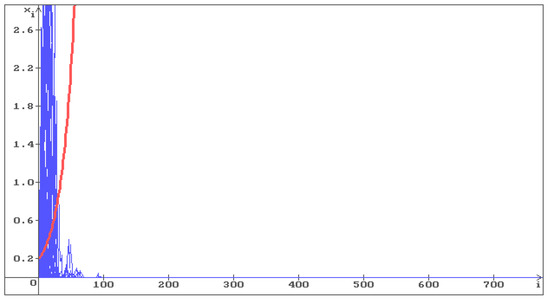
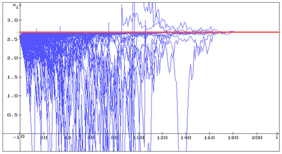
To illustrate Hypothesis 1, consider Equation (6) with $a_1=1.05$, $x_0=0.2$. In Figure 1, Figure 2 and Figure 3, 100 trajectories (blue) of the solution of Equation (6) are shown, respectively, with ${\sigma }_1=0.2$, ${\sigma }_1=0.3$ and ${\sigma }_1=0.4$. The red line corresponds to the deterministic case ${\sigma }_1=0$.

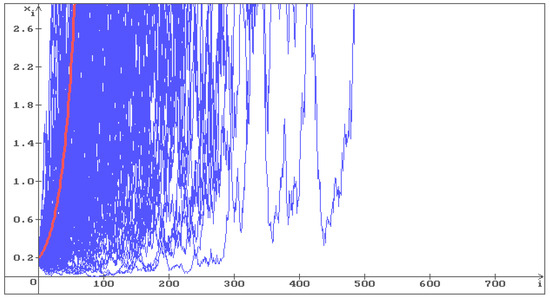
Figure 1. 100 trajectories (blue) of the solution $x_i$ of Equation (6) with $a_1=1.05$, ${\sigma }_1=0.2$. The equilibrium $x^{*}=0$ is unstable, all trajectories with $x_0=0.2$ go to infinity. The red line corresponds to the deterministic case, i.e., ${\sigma }_1=0$.

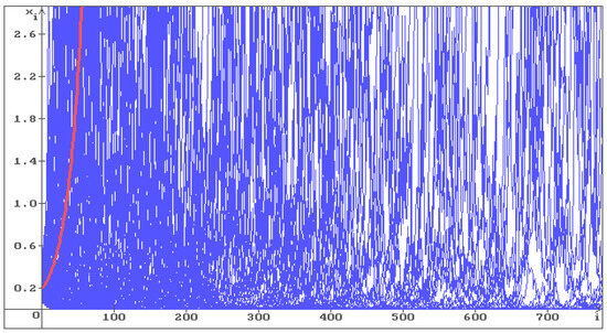
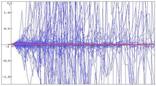
Figure 2. 100 trajectories (blue) of the solution $x_i$ of Equation (6) with $a_1=1.05$, ${\sigma }_1=0.3$. The equilibrium $x^{*}=0$ is unstable, all trajectories with $x_0=0.2$ fill whole space. The red line corresponds to the deterministic case, i.e., ${\sigma }_1=0$.

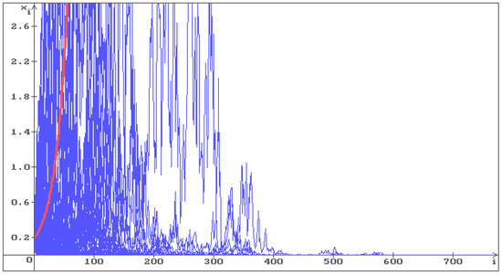
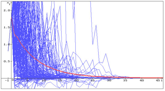
Figure 3. 100 trajectories (blue) of the solution $x_i$ of Equation (6) with $a_1=1.05$, ${\sigma }_1=0.4$. Stabilization by noise occurs and all trajectories with $x_0=0.2$ converge to $x^{*}=0$. The red line corresponds to the deterministic case, i.e., ${\sigma }_1=0$.

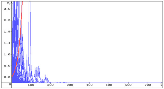
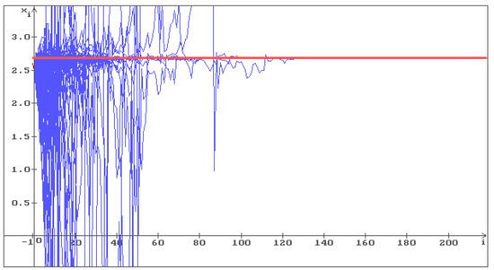
One can see that in Figure 1, all trajectories go to infinity, and in Figure 2 the trajectories fill the whole space. In Figure 3, where the condition (12) holds $(2(a_1-1)=0.1<{\sigma }_1^2=0.16)$, the stabilization by noise occurs and all trajectories converge to the stable equilibrium $x^{*}=0$. As the noise intensity increases, the trajectories converge to $x^{*}=0$ faster: in Figure 4 ${\sigma }_1=0.5$, in Figure 5 ${\sigma }_1=0.6$.

Figure 4. 100 trajectories (blue) of the solution $x_i$ of Equation (6) with $a_1=1.05$, ${\sigma }_1=0.5$. Noise level has increased, all trajectories with $x_0=0.2$ converge to $x^{*}=0$ faster than in Figure 3. The red line corresponds to the deterministic case, i.e., ${\sigma }_1=0$.

Figure 5. 100 trajectories (blue) of the solution $x_i$ of Equation (6) with $a_1=1.05$, ${\sigma }_1=0.6$. Noise level has increased, all trajectories with $x_0=0.2$ converge to $x^{*}=0$ faster than in Figure 4. The red line corresponds to the deterministic case, i.e., ${\sigma }_1=0$.

Thus, the hypothesis about stabilization by noise for stochastic difference equations is confirmed by numerical simulation of solutions of the linear stochastic difference Equation (6).

3. Nonlinear Stochastic Difference Equation

As an example of a nonlinear difference equation, consider the so-called bilinear difference equation. During the last two decades, rational difference equations, in particular, rational bilinear difference equations have become very popular in research (see, for instance, [8] and references therein). In particular, stability of the bilinear difference equation.

$$\begin{gathered} x_{n+1}=a{x}_n+\frac{b{x}_n{x}_{n-1}}{c{x}_n+d{x}_{n-1}},n\in Z, \\ {x}_n={\varphi }_n,n\in Z_0, \end{gathered}$$

with positive parameters $a,b,c,d$ and initial values ${\varphi }_{-1}$, ${\varphi }_0$ is studied in [8].

It is clear that, without loss of generality, one of the parameters $b,c,d$ in this equation can be equated to 1. Let $d=1$. So, we will consider the bilinear difference equation

$$\begin{gathered} x_{n+1}=a{x}_n+\frac{b{x}_n{x}_{n-1}}{c{x}_n+x_{n-1}},n\in Z, \\ {x}_n={\varphi }_n,n\in Z_0, \end{gathered}$$

(13)

with positive $a,b,c$ and ${\varphi }_{-1}$, ${\varphi }_0$.

The following two statements, obtained in [8], for Equation (13) take the form:

Statement 1. 

If $(1-a)(c+1)\ne b$ then the unique equilibrium of Equation (13) is $x^{*}=0$.

Statement 2. 

If $(1-a)(c+1)>b$ then the zero solution of Equation (13) is locally asymptotically stable.

3.1. Equilibria of Equation (13)

Putting $x_n=x^{*}$ for $n\ge -1$, we obtain that the equilibrium $x^{*}$ of Equation (13) is defined by the equation

$$x^{*}\left(1-a-\frac{b}{c+1}\right)=0.$$

(14)

It is clear that if

$$a+\frac{b}{c+1}\ne 1$$

(15)

then $x^{*}=0$ only can be the equilibrium of Equation (13) (that coincides with Statement 1).

From the other hand, by the assumption

$$a+\frac{b}{c+1}=1$$

(16)

each $x^{*}\in \mathbf{R}$ is a solution of Equation (14) and $x_n=x^{*}$, $n\ge -1$, is a solution of Equation (13).

Remark 2. 

Note that by the condition (16) from the equality $x_m=x_{m-1}=x^{*}$ for some $m\ge 0$ from (13) it follows that $x_n=x^{*}$ also for all $n>m$.

Note that via Remark 2 by the condition (16) and $x_0=x_{-1}$ Equation (13) has the equilibrium $x^{*}=x_0$. Let us assume that Equation (13) is exposed to stochastic perturbations that are directly proportional to the deviation of the solution $x_n$ from the equilibrium $x^{*}$, i.e., Equation (13) takes the form of the stochastic difference Equation [7]

$$x_{n+1}=a{x}_n+\frac{b{x}_n{x}_{n-1}}{c{x}_n+x_{n-1}}+\sigma (x_n-x^{*}){\xi }_{n+1},n\in Z,$$

(17)

where $\sigma$ is a constant. By that the solution $x_n=x^{*}$ of Equation (13) is also the solution of Equation (17).

Remark 3. 

Note that stochastic perturbations of the type (17) were first used for a system of stochastic delay differential equations in [9] and later in many other different research both for differential and for difference equations (see, for instance, [6,7] and references therein).

Putting in (17) $x_n=y_n+x^{*}$, we obtain

$$y_{n+1}=a(y_n+x^{*})-x^{*}+\frac{b(y_n+x^{*})(y_{n-1}+x^{*})}{c(y_n+x^{*})+y_{n-1}+x^{*}}+\sigma y_n{\xi }_{n+1}$$

or

$$y_{n+1}=a{y}_n+(a-1)x^{*}+\frac{b[{\left(x^{*}\right)}^2+(y_n+y_{n-1})x^{*}+y_n{y}_{n-1}]}{(c+1)x^{*}+c{y}_n+y_{n-1}}+\sigma y_n{\xi }_{n+1}.$$

(18)

Lemma 1. 

Let the condition (16) hold and $x^{*}\ne 0$. The linear part of Equation (18) then has the form

$$\begin{gathered} z_{n+1}=\alpha z_n+\beta z_{n-1}+\sigma z_n{\xi }_{n+1},n\in Z, \\ {z}_n={\varphi }_n,n\in Z_0, \end{gathered}$$

(19)

where

$$\alpha =a+\frac{b}{{(c+1)}^2},\beta =\frac{bc}{{(c+1)}^2},\alpha +\beta =1.$$

(20)

Proof. 

Using the equality

$${\displaystyle \frac{1}{p+y}}={\displaystyle \frac{1}{p}}-{\displaystyle \frac{y}{p^2}}+o\left(y\right),\mathrm{where}p\ne 0\mathrm{and}\underset{y\to 0}{lim}{\displaystyle \frac{o\left(y\right)}{y}}=0,$$

we have

$$\begin{array}{l}\frac{b[{\left(x^{*}\right)}^2+(y_n+y_{n-1})x^{*}+y_n{y}_{n-1}]}{(c+1)x^{*}+c{y}_n+y_{n-1}}\\ =b[{\left(x^{*}\right)}^2+(y_n+y_{n-1})x^{*}+y_n{y}_{n-1}]\left(\frac{1}{(c+1)x^{*}}-\frac{c{y}_n+y_{n-1}}{{(c+1)}^2{\left(x^{*}\right)}^2}+o\left(y\right)\right)\\ =\frac{b{x}^{*}}{c+1}-\frac{b}{{(c+1)}^2}(c{y}_n+y_{n-1})+\frac{b}{c+1}(y_n+y_{n-1})+o\left(y\right).\end{array}$$

(21)

Substituting (21) into (18), neglecting the nonlinear terms and using (14), we obtain

$$\begin{array}{ll}{z}_{n+1}& =a{z}_n+(a-1)x^{*}+\frac{b{x}^{*}}{c+1}-\frac{b}{{(c+1)}^2}(c{z}_n+z_{n-1})+\frac{b}{c+1}(z_n+z_{n-1})+\sigma z_n{\xi }_{n+1}\\ & =\left(a-1+\frac{b}{c+1}\right)x^{*}+\left(a+\frac{b}{c+1}-\frac{bc}{{(c+1)}^2}\right)z_n+\left(\frac{b}{c+1}-\frac{b}{{(c+1)}^2}\right)z_{n-1}+\sigma z_n{\xi }_{n+1}\\ & =\left(a+\frac{b}{{(c+1)}^2}\right)z_n+\frac{bc}{{(c+1)}^2}{z}_{n-1}+\sigma z_n{\xi }_{n+1},\end{array}$$

that via (20) gives (19). In addition, the equality $\alpha +\beta =1$ coincides with (16). The proof is completed. □

3.2. Stability

Definition 3. 

The zero solution of Equation (18) is called stable in probability if for any $\epsilon >0$ and ${\epsilon }_1\in (0,1)$ there exists a $\delta >0$ such that the solution $y_n$ of Equation (18) satisfies the inequality $\mathbf{P}\{\underset{n\in Z}{sup}|y_n|>\epsilon /{\mathfrak{F}}_0\}<{\epsilon }_1$ for any initial function ϕ such that $\mathbf{P}\{\underset{n\in Z_0}{max}|{\varphi }_n|<\delta \}=1$.

Definition 4. 

The zero solution of Equation (19) is called:

• - mean square stable if for each $\epsilon >0$ there exists a $\delta >0$ such that $\mathbf{E}{z}_n^2<\epsilon$, $n\in Z$, for any initial function $\varphi \left(n\right)$ such that ${\parallel \varphi \parallel }^2=\underset{n\in Z_0}{max}\mathbf{E}{\left|\varphi \left(n\right)\right|}^2<\delta$;
• - asymptotically mean square stable if it is mean square stable and for each initial function $\varphi \left(n\right)$ such that ${\parallel \varphi \parallel }^2<\infty$ the solution $z_n$ of Equation (19) satisfies the condition $\underset{n\to \infty }{lim}\mathbf{E}{z}_n^2=0$.

Remark 4. 

It is clear that stability of the equilibrium $x^{*}$ of Equation (17) is equivalent to stability of the zero solution of Equation (18). It is known [7] that the investigation of stability in probability of the zero solution of a nonlinear stochastic difference equation with an order of nonlinearity higher than one can be reduced to the investigation of asymptotic mean square stability of the zero solution of the linear part of this equation. So, to obtain conditions for stability in probability of the equilibrium $x^{*}$ of the nonlinear stochastic difference Equation (17) it is enough to get conditions for asymptotic mean square stability of the zero solution of the linear stochastic difference Equation (19) that in the case of $x^{*}\ne 0$ is the linear part of the nonlinear difference Equation (18).

Lemma 2. 

[7] If

$$\left|\alpha \right|+\left|\beta \right|<\sqrt{1-{\sigma }^2}$$

(22)

then the zero solution of Equation (19) is asymptotically mean square stable.

Lemma 3. 

[7] The inequalities

$$\left|\beta \right|<1,\left|\alpha \right|<1-\beta ,{\sigma }^2<\frac{1+\beta }{1-\beta }\left[{(1-\beta )}^2-{\alpha }^2\right],$$

(23)

are the necessary and sufficient conditions for asymptotic mean square stability of the zero solution of Equation (19).

Remark 5. 

Note that the stability conditions (22) and (23) are obtained via the general method of Lyapunov functionals construction [7].

Example 1. 

Put in Equation (17) $a=0.5$, $b=0.7$, $c=1$, $\sigma =0.5$. The condition (22) holds: $a+{\displaystyle \frac{b}{c+1}}=0.85<\sqrt{1-{\sigma }^2}=0.866$. Besides, the conditions (22) and (23) give, respectively, ${\sigma }^2<0.28$ and ${\sigma }^2<0.32$. In Figure 6, 500 trajectories (blue) of the solution of Equation (17) are shown with the initial conditions $x_{-1}=0.8$, $x_0=1.8$ and the stable equilibrium $x^{*}=0$. One can see that all trajectories converge to the stable equilibrium $x^{*}=0$. Note that this corresponds to Statement 2.

Figure 6. 500 trajectories (blue) of the solution $x_n$ of Equation (17) with $a=0.5$, b = $0.7$, $c=1$, $\sigma =0.5$, $x_{-1}=0.8$, $x_0=1.8$ and stable equilibrium $x^{*}=0$. The red line corresponds to the deterministic case, i.e., $\sigma =0$.

Now place $\sigma =0.95$ with the same values of all other parameters. The conditions (22) and (23) do not hold. In Figure 7, 500 trajectories (blue) of the solution of Equation (17) with $x^{*}=0$ are shown with the initial conditions $x_{-1}=0.01$, $x_0=0.02$. The zero solution is unstable and the trajectories fill the whole space.

Figure 7. 500 trajectories (blue) of the solution $x_n$ of Equation (17) with $a=0.5$, b = $0.7$, $c=1$, $\sigma =0.95$, $x_{-1}=0.01$, $x_0=0.02$ and unstable equilibrium $x^{*}=0$. The red line corresponds to the deterministic case, i.e., $\sigma =0$.

The red lines in the both Figure 6 and Figure 7 correspond to the deterministic case, i.e., $\sigma =0$.

Remark 6. 

Note that by the conditions (22) and (23) the condition (15) holds, by which Equation (13) has the equilibrium $x^{*}=0$ only. However, the linear Equation (19) is obtained by the conditions (16) and $x^{*}\ne 0$. Thus, strictly speaking, Equation (19) cannot be used for studying the zero equilibrium. So, below the equilibrium $x^{*}\ne 0$ is considered.

Example 2. 

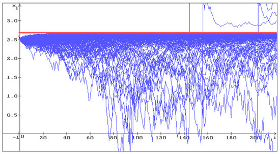
Put $a=0.65$, $b=0.7$, $c=1$, $\sigma =0.15$, $x^{*}=2.7$. Wherein $a+{\displaystyle \frac{b}{c+1}}=1$, therefore, the condition (16) holds, the conditions (22) and (23) do not hold. In Figure 8, the red straight corresponds to the constant solution $x_n=x^{*}$, $n\ge -1$, 500 trajectories (blue) of the solution of Equation (17) are shown with the initial conditions $x_{-1}=x^{*}-0.1=2.6$, $x_0=x^{*}-0.2=2.5$. The solution $x_n=x^{*}$ is unstable, so, the trajectories fill the whole space.

Figure 8. 500 trajectories (blue) of the solution $x_n$ of Equation (17) with $a=0.65$, b = $0.7$, $c=1$, $\sigma =0.15$, $x_{-1}=2.6$, $x_0=2.5$ and unstable equilibrium $x^{*}=2.7$. The red straight corresponds to the constant solution $x_n=x^{*}$, $n\ge -1$, $\sigma =0$.

Put now $\sigma =0.45$ with the same values of all other parameters. In Figure 9, one can see that all 500 trajectories converge to the solution $x_n=x^{*}=2.7$ of Equation (17). Putting $\sigma =0.75$, i.e., increasing once more the level of noise, we obtain (see Figure 10) that all 500 trajectories converge to the solution $x_n=x^{*}=2.7$ of Equation (17) faster than in Figure 9. So, the solution $x_n=x^{*}=2.7$ of Equation (17), that is unstable by the small level of noise ($\sigma =0.15$), becomes stable by increasing the level of noise, i.e., stabilization by noise occurs.

Figure 9. 500 trajectories (blue) of the solution $x_n$ of Equation (17) with $\sigma =0.45$ and the same values of all other parameters as in Figure 8. All trajectories converge to the stable equilibrium $x^{*}=2.7$.

Figure 10. 500 trajectories (blue) of the solution $x_n$ of Equation (17) with $\sigma =0.75$ and the same values of all other parameters as in Figure 8. All trajectories converge to the stable equilibrium $x^{*}=2.7$ faster than in Figure 9.

4. Conclusions

The very important problem of “stabilization by noise”, which for more than 50 years has been well known for stochastic differential equations, is studied here for stochastic difference equations. Via numerical simulation of solutions of linear and nonlinear stochastic difference equations, the hypothesis about a possibility of stabilization by noise is demonstrated and confirmed also for stochastic difference equations. However, a formal proof of this hypothesis remains until now an unsolved problem.

References

- Gikhman, I.I.; Skorokhod, A.V. Introduction to the Theory of Random Processes; Saunders: Philadelphia, PA, USA, 1969. [Google Scholar]
- Gikhman, I.I.; Skorokhod, A.V. Stochastic Differential Equations; Springer: Berlin, Germany, 1972. [Google Scholar]
- Gikhman, I.I.; Skorokhod, A.V. The Theory of Stochastic Processes; Springer: Berlin, Germany, 1974; Volume I, 1975; Volume II, 1979, Volume III. [Google Scholar]
- Shaikhet, L. Some unsolved problems in stability and optimal control theory of stochastic systems (Special Issue “Models of Delay Differential Equations—II”). Mathematics 2022, 10, 474. [Google Scholar] [CrossRef]
- Khasminskii, R.Z. Stochastic Stability of Differential Equations; Springer: Berlin, Germany, 2012. [Google Scholar]
- Shaikhet, L. Lyapunov Functionals and Stability of Stochastic Functional Differential Equations; Springer Science & Business Media: Berlin, Germany, 2013. [Google Scholar]
- Shaikhet, L. Lyapunov Functionals and Stability of Stochastic Difference Equations; Springer Science & Business Media: London, UK, 2011. [Google Scholar]
- Elsayed, E.M. Qualitative behavior of a rational recursive sequence. Indag. Math. 2008, 19, 189–201. [Google Scholar] [CrossRef][Green Version]
- Beretta, E.; Kolmanovskii, V.; Shaikhet, L. Stability of epidemic model with time delays influenced by stochastic perturbations. Math. Comput. Simul. 1998, 45, 269–277. [Google Scholar] [CrossRef]
Disclaimer/Publisher’s Note: The statements, opinions and data contained in all publications are solely those of the individual author(s) and contributor(s) and not of MDPI and/or the editor(s). MDPI and/or the editor(s) disclaim responsibility for any injury to people or property resulting from any ideas, methods, instructions or products referred to in the content. |
© 2023 by the author. Licensee MDPI, Basel, Switzerland. This article is an open access article distributed under the terms and conditions of the Creative Commons Attribution (CC BY) license (https://creativecommons.org/licenses/by/4.0/).