Article

A Coupled Machine Learning and Lattice Boltzmann Method Approach for Immiscible Two-Phase Flows

1
School of Advanced Manufacturing, Nanchang University, Nanchang 330031, China
2
Institute of Energy and Sustainable Development (IESD), School of Engineering and Sustainable Development, De Montfort University, Leicester LE1 9BH, UK
*
Authors to whom correspondence should be addressed.
Mathematics 2024, 12(1), 109; https://doi.org/10.3390/math12010109
Submission received: 14 November 2023 / Revised: 16 December 2023 / Accepted: 26 December 2023 / Published: 28 December 2023

Abstract

:
An innovative coupling numerical algorithm is proposed in the current paper, the front-tracking method–lattice Boltzmann method–machine learning (FTM-LBM-ML) method, to precisely capture fluid flow phase interfaces at the mesoscale and accurately simulate dynamic processes. This method combines the distinctive abilities of the FTM to accurately capture phase interfaces and the advantages of the LBM for easy handling of mesoscopic multi-component flow fields. Taking a single vacuole rising as an example, the input and output sets of the machine learning model are constructed using the FTM’s flow field, such as the velocity and position data from phase interface markers. Such datasets are used to train the Bayesian-Regularized Back Propagation Neural Network (BRBPNN) machine learning model to establish the corresponding relationship between the phase interface velocity and the position. Finally, the trained BRBPNN neural network is utilized within the multi-relaxation LBM pseudo potential model flow field to predict the phase interface position, which is compared with the FTM simulation. It was observed that the BRBPNN-predicted interface within the LBM exhibits a high degree of consistency with the FTM-predicted interface position, showing that the BRBPNN model is feasible and satisfies the accuracy requirements of the FT-LB coupling model.

1. Introduction

A mesoscale multiphase flow characterized by intricate fluid dynamics is a prevalent flow phenomenon in both natural and engineering systems, occupying an intermediate position between macro and micro scales. It serves as the fundamental basis for the survival of numerous organisms in nature and plays a crucial role in various interdisciplinary and multidisciplinary applications. Interface properties, such as viscous shear force and surface tension, play a pivotal role in the flow process at the mesoscale. Moreover, the physical and chemical parameters of the interface, along with complex structural geometric parameters at the pore scale, exert significant influences on the study of dynamic characteristics of interfaces. Therefore, it is crucial for related research to employ numerical methods that can accurately and efficiently compute the evolution process of multi-component multiphase interfaces in complex geometric structures. Yuan et al. [1] used VOF simulations to study the multi-hopping phenomenon, which provides an effective guideline for the design of an SHS with an enhanced droplet hopping function and thus is widely used in industry. Lin et al. [2] investigated the effect of fluid shear on bubble distribution in a channel flow with a periodically oscillating pressure gradient by direct numerical simulation. In addition, external forces such as electric field forces cannot be neglected. Lu et al. [3] investigated the effect of electrostatic forces on the distribution of water droplets in a turbulent channel flow through direct numerical simulations. The results show that the applied electric field has a significant effect on the microstructure and flow characteristics.
Tryggvason et al. [4,5] proposed a new interface tracking method, the front-tracking method (FTM), for labeling the phase interface and explicitly tracking the interface movement process, which uses the Lagrange method to label the phase interface’s movements over time. The Lagrange interface marks are connected to each other to describe the continuous phase interface, and the Euler grid points are calculated to transfer the physical quantity to the interface marks. Since the interface is displayed, the physical quantity of each interface mark can be accurately obtained. Therefore, the evident advantages of the FTM are the more accurate capture and tracking of the phase interface, the thinner phase interface thickness, clearer interface, and more accurate calculations of surface tension. Li et al. [6] used a numerical model based on FTM to study the self-migrating motion of droplets on a wetting gradient surface, and found that the transport mode of droplets on a discontinuous wetting gradient surface depends on the surface roughness. Lu et al. [7] studied the deformation of bubbles in a turbulent basin, and the results showed that the deformation of bubbles could significantly reduce the viscous resistance of walls by suppressing vorticity. Lu et al. [8] studied the influence of obstacles in the channel on the thermal capillary migration of deformable bubbles and found that obstacles had a greater impact on bubble velocity in the two-dimensional case. Juric et al. [9] accurately described the phase interface evolution process of film boiling by introducing a latent heat source term and verified the accuracy of the model through observations of and comparisons between experimental results and the heat transfer calculations. Through the research and optimization performed by various scholars, the FTM has gradually developed and matured, and has become the mainstream algorithm in interface labeling.
In the 20th century, scholars proposed the lattice Boltzmann method [10,11,12] (LBM), which is a mesoscopic scaling method based on the minimum lattice formula of the Boltzmann equation of kinetics. After a series of research works, the Multiple Relaxation Time (MRT) matrix collision model was gradually optimized [13], which greatly improved the computational stability and accuracy. For more complex multiphase flow problems, Shan and Chen (S-C) [14] proposed a multiphase LBM model, that is, a pseudo-potential model, which uses the interaction between microscopic particles as the external force term in the LBM equation and realizes the separation between phases according to the mutual attraction of the same kind of particles. In terms of the expression of force, the traditional S-C format [14], EDM format [15] and Guo format [16] were further optimized by Li et al. [17]. For the gas equation of state, Kupershtokh et al. [18] also conducted a series of research and optimization studies. At the same time, Yu et al. [19,20] introduced the MRT equation into the pseudo-potential model to replace the original BGKW approximate equation, which further improved the accuracy of solving the multiphase flow problem. To date, the MRT-LBM pseudo-potential model has been considered the most efficient and easy-to-solve solution to parallel complex multi-component multiphase flow field problems. However, in the process of solving the flow field, mass interaction gradient bands of a certain thickness will be generated between the grid points of two adjacent components of the fluid, and a smooth transition of the phase interface cannot be realized, which restricts the wide use of the LBM.
Therefore, in order to solve multiphase flow problems at the mesoscale with high-precision interface capture and a high efficiency, a numerical simulation method combining the FTM and LBM was proposed. Lallemand et al. [21] proposed combining the lattice Boltzmann equation (LBE) and the front-tracking method (FTM) to simulate interfacial dynamics with surface tension in two dimensions (2D). Sui et al. [22] adopted the multi-block strategy of the multi-block lattice Boltzmann method to refine the mesh covering the area near the capsule to calculate different physical properties of the fluid, used the FTM to display the membrane nodes tracking the capsule membrane, and introduced the finite element model to describe the membrane mechanics. Xie et al. [23] adopted the flow field of the three-dimensional multi-relaxation collision LBM in the Euler mesh, adopted the FTM-adapted unstructured triangular Lagrange mesh, explicitly tracked the motion of the interface of the two fluids, and accurately updated the physical properties of the fluids through the indication function.
With the development of science and technology, various disciplines and fields have gradually become reliant on multidimensional and high-demand analyses of a large amount of data, and machine learning is widely used in many fields. Yuan et al. [24] experimentally proposed enhanced jumping methods, used machine learning to design structures that achieve ultimate jumping, and finally combined experiments and simulations to investigate the mechanism of enhanced jumping. Yuan et al. [25] proposed a method of controlling the jumping direction through the surface structure by varying the tilt angle of the structure and therefore developed a more comprehensive predictive model based on a convolutional neural network (CNN) to predict the jumping direction in more general cases. On this basis, Bishop et al. [26] used machine learning to complete the determination of components in multiphase fluids. Milanoet et al. [27] applied proper orthogonal decomposition to linear grids, proposed a nonlinear neural network extension method, and applied it to the study of flow processes and the reconstruction of the turbulent flow field in near-wall regions. Ma et al. [28] built a two-branch Deep Neural Network (TBDNN) model to improve the results of high-fidelity bubble migration and further reduce the dependence on the amount of experimental data. Han et al. [29] designed a novel hybrid Deep Neural Network (DNN) architecture to directly capture the spatiotemporal characteristics of unsteady flows from high-dimensional numerical unsteady flow field data. In order to reduce the computational cost of solving the Navier–Stokes equations, some researchers have applied machine learning to the iterative solution of these equations. Chen et al. [30] proposed a machine-learning-based method to solve the large-scale Poisson equation and verified the effectiveness of this method through different solutions, which showed how scientific computing can utilize machine learning to improve simulation without sacrificing accuracy or the generalization ability. Brenner et al. [31] offer a perspective on how machine learning is advancing fluid dynamics; the success of machine learning will depend in part on the availability of training data, which are difficult to obtain from high-fidelity simulations or experiments. Many ML algorithms require large amounts of data in order to reduce errors to appropriately low values, which is the main limitation of machine learning. However, as long as the same high standard is applied to the discovery of any generalizable understanding, the risk is low.
All of the above coupling algorithms only solve the flow field via the LBM, and then substitute the LBM velocity field into the FTM to update the velocities and positions on the interface points, realizing the explicit tracking of the interface points. However, the FTM will automatically update the interface marker points when realizing the accurate evolution of the phase interface, and when the phase interface is fused or ruptured, it is necessary to manually set the conditions for adding or deleting marker points, which will lead to a slight lack of mass conservation at the interface. Thus, there is the problem of a lack of mass conservation in the explicit tracking of the evolution of the phase interface via the FTM, and this will affect the accuracy of the simulation to a certain extent. Secondly, although machine learning has more applications and is a powerful tool in fluid mechanics research, it has not yet been applied to the coupling of two algorithms: the FTM and LBM. The core idea of this algorithm is to mark the phase interface with the lattice unit thickness in the LBM by using the interface point marking in the FTM, and the marking process is implemented by using a neural network model based on machine learning, thus realizing the marking of the interface points in the LBM by obtaining the intrinsic functional relationship between the flow field information and the interface information in the FTM. This makes the phase interface in the flow field of the LBM clearer and more accurate; however, the optimized flow field is not involved in the whole calculation cycle to ensure the mass conservation over the whole calculation process. The physical information of the flow field and the phase field is realized by the multi-relaxation lattice Boltzmann multiphase pseudopotential model. Since the multi-relaxation lattice Boltzmann multiphase pseudopotential model has the advantage of automatically generating and evolving phase interfaces, the updating of the flow field can be realized more easily and efficiently and the pseudopotential model can be coupled with the FTM to better simulate fluid systems with multicomponent, multiphase interfacial dynamics (e.g., multiphase flow, interfacial phenomena) compared with the single-phase, single-component LBM.

2. Method

2.1. Governing Equations of the Front-Tracking Method

Assuming that the fluid is incompressible, the mass conservation equation can be expressed as:
u = 0
where u is the velocity vector. The momentum equation is:
ρ u t = ρ u u p + ρ g + μ u + T u + F
where ρ is the fluid density, t is the time, p is the pressure, g is the acceleration of gravity, μ is the dynamic viscosity of the fluid, and F is the surface forces.
F = Γ σ κ n δ x x f d s
By separating the pressure term in Equation (2) from the other terms and introducing the temporary velocity u*, we can obtain:
ρ n + 1 u * ρ n u n Δ t = ρ n u n u n + ρ n g + μ n u n + T u n + F
The process of solving the Navier–Stokes equation follows the projection method [32,33], where n represents a certain moment, n + 1 is the next moment of n moment, and Δ t is the time step. The central difference scheme is used for the discretization of the diffusion term on the right side of the above equation, and the QUICK (Quadratic Upstream Interpolation for Convective Kinetics) format is used for the convection term to obtain the temporary velocity u*, which is then brought into the pressure term to obtain the actual velocity un+1. The following can then be obtained:
ρ n + 1 u n + 1 ρ n + 1 u * Δ t = h p
where h is the Hamiltonian operator with step size h. The divergence between the left and right sides of the above formula can be obtained:
ρ n + 1 u n + 1 ρ n u * Δ t = h 2 p
The pressure Poisson equation can be obtained by combining the above equation with mass conservation Equation (1).
h u * Δ t = h 1 ρ n + 1 h p
The above equation can be solved by over-relaxation iteration (SOR) to obtain the pressure p, which can be put into Equation (5) to obtain:
u n + 1 = u * Δ t ρ n + 1 h p
After obtaining the actual velocity un+1 at time n + 1, the above process can be repeated so as to obtain n + 2, n + 3, etc.; the actual velocity at all times.

2.2. Marking and Tracing of Interfaces

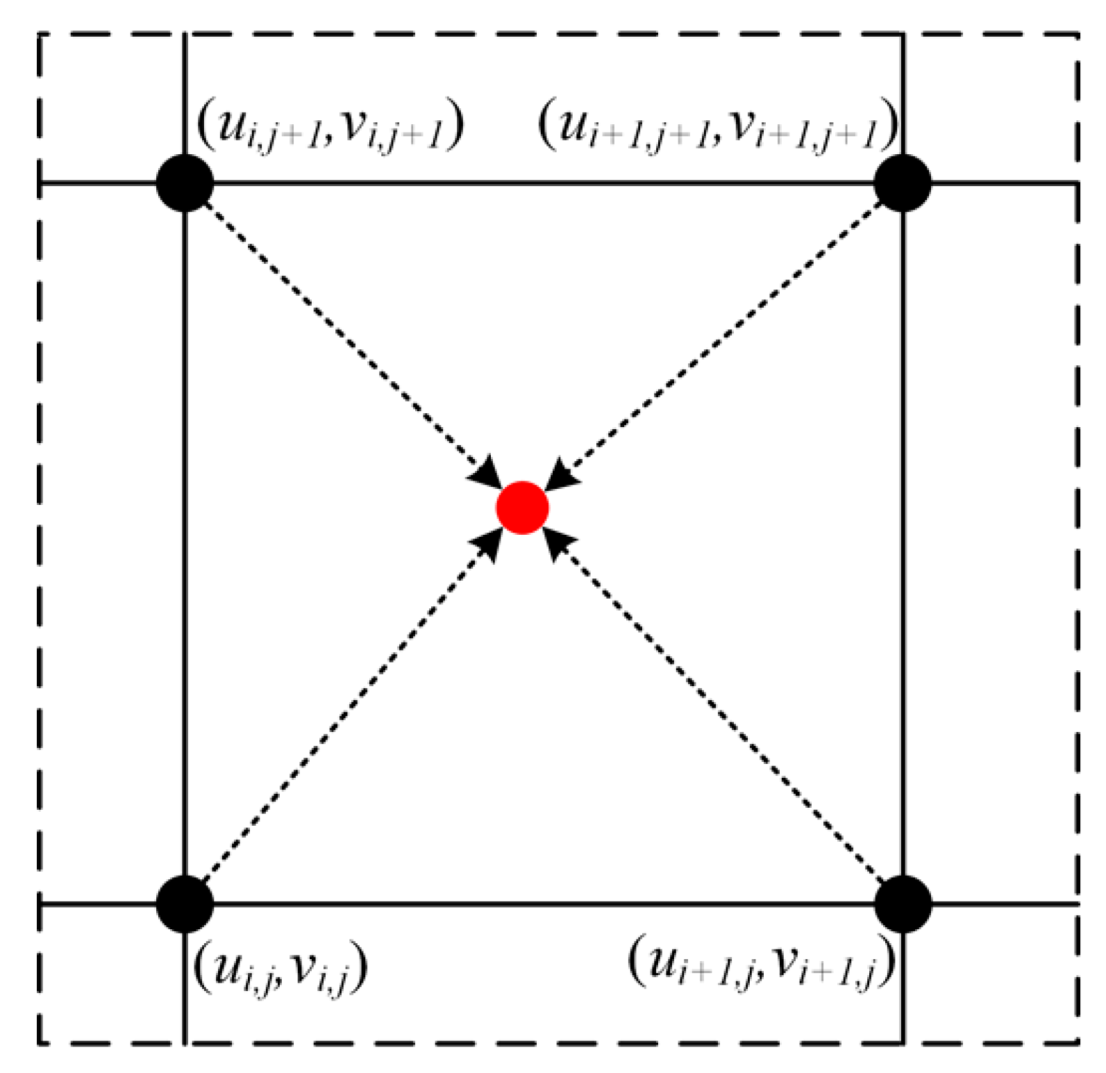
The interface marker points are not restricted to the Eulerian staggered grid described above, but are Lagrangian points with time as the independent variable, allowing for a maximally realistic and smooth description of the interface. In order to make the interface move over time in the calculation, it is necessary to calculate the speed of each interface marker. The coordinates of the interface markers do not coincide with the Eulerian grid points in the flow field, so it is necessary to interpolate the velocity information of the Euler staggered grid points to obtain the velocity of the interface markers. As shown in Figure 1, the black point represents the Euler grid point and the blue and red points represent the interface. When calculating the velocity of the red interface mark point in the figure, the four grid points closest to the interface point should be taken as reference, and the velocity at the four grid points should be interpolated to the red interface point by using the area interpolation method with corresponding weights. One can obtain the velocity at that point.
For the weighting coefficients w i , j l , they need to satisfy:
i , j w i , j l = 1
This also needs to be satisfied in order to ensure that the physical quantities are conserved before and after discretization:
Δ l ϕ f l d l = Δ s ϕ i , j x d s
where Δ l is the length of the interface distributed into the surrounding area Δ s obtained after discretization:
ϕ i , j = l w i , j l ϕ i , j Δ l Δ x Δ y
In order to define the fluid density and determine the interface position, the Heaviside function is defined by density jump.
H = 1 f l u i d 1 0 f l u i d 2
The density is written as:
ρ = ρ 1 H + 1 H ρ 2

2.3. Lattice Boltzmann Method Modeling

For the overall motion process of the particle distribution function f(r, C, t) in a fluid in time and space, the general total differential expression of the lattice Boltzmann equation is as follows:
d f d t = f r C + f C a + f t
where r is the position coordinate of the particle, C is the motion velocity of the particle, a is the acceleration of the particle, and t is the time. Ideally, the BGKW approximation can be introduced:
f t = 1 γ f e q f
where γ is the relaxation time and f e q is the equilibrium distribution function. Combining Equations (14) and (15) and discretizing the time term and space phase, the following can be obtained:
f α ( x + e α δ t , t + δ t ) = f α ( x , t ) 1 γ f α ( x , t ) f α e q ( x , t )
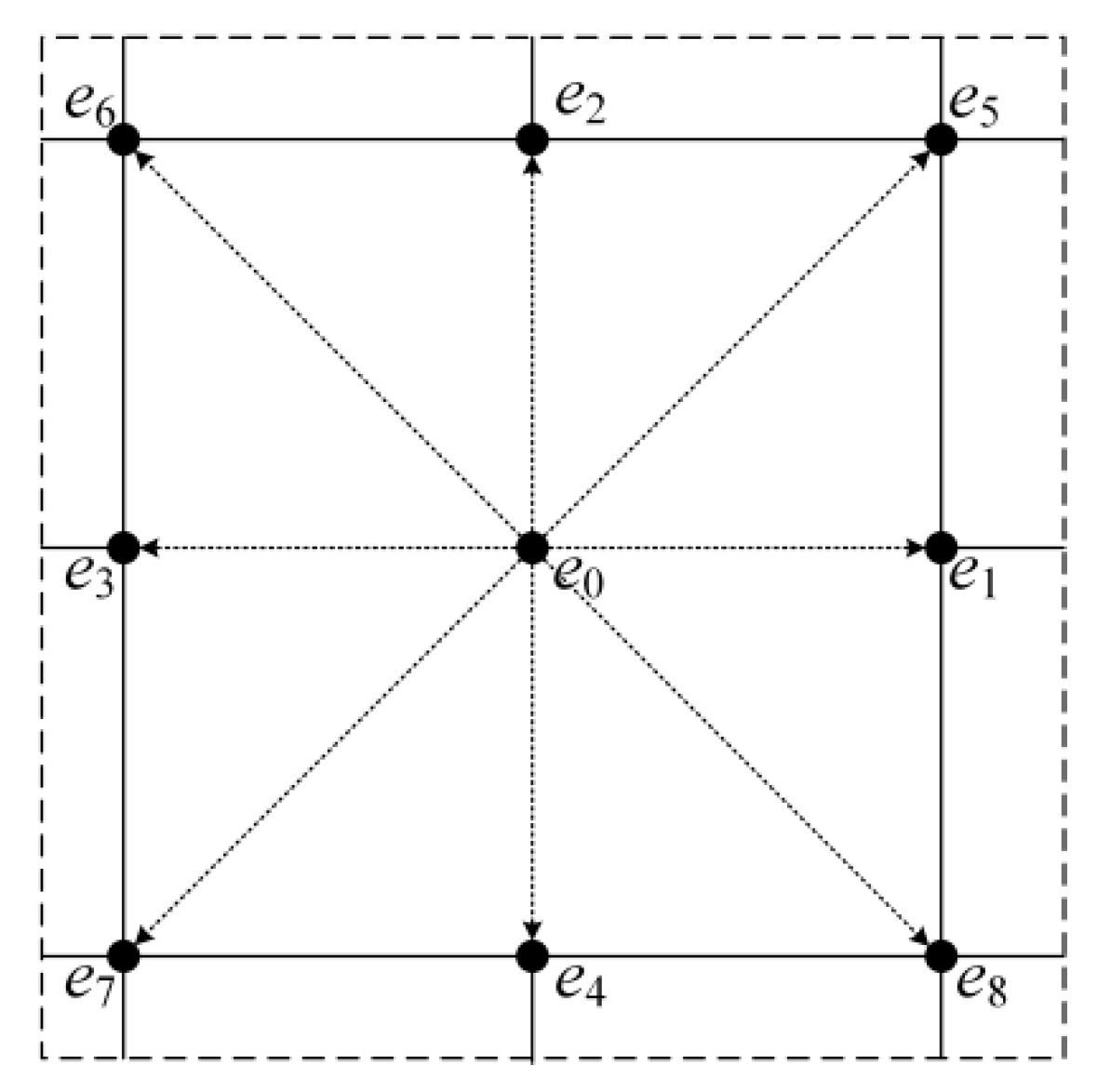
where e α is the discrete velocity in the direction α , δ t is the particle movement time, f α is the particle distribution function in the direction α , and f α e q is the particle distribution function at the equilibrium time in the direction α . The present work employs a D2Q9 LBM model; i.e., the discrete velocities are spatially labeled in nine velocities, as shown in Figure 2, and the discrete velocities can be expressed as:
e i = ( 0 , 0 ) , i = 0 ( 1 , 0 ) c , ( 0 , 1 ) c , ( 1 , 0 ) c , ( 0 , 1 ) c , i = 1 4 ( 1 , 1 ) c , ( 1 , 1 ) c , ( 1 , 1 ) c , ( 1 , 1 ) c , i = 5 8
c = Δ x Δ t
where Δ x is the space step and Δ t is the time step. Then, c is the lattice velocity, and both Δ x and Δ t area 1 during the simulation in the current study.
In the pseudo-potential model, Shan and Chen proposed an interaction force between particles to describe the separation process of two terms. The interaction force F = F x , F y between particles in the S-C model can be expressed as:
F = G ψ ( x ) α = 1 8 ω ( e α 2 ) ψ ( x + e α ) e α
where G is the strength of interaction, which is positive or negative depending on the attractive or repulsive force between the particles; ω e α 2 is the weight factor of interaction, where in the D2Q9 model, ω 1 is 1/3 and ω 2 is 1/12; and ψ is the effective interaction potential energy, namely the pseudo-potential energy, which can be expressed as follows:
ψ = ρ 0 ( 1 e ρ ρ 0 )
where ρ 0 is a normalization constant, usually taken as 1. Describing the interaction force between particles in terms of an ideal gas equation of state with external forces gives:
p x + ( c s 2 ρ ) y = F y

2.4. Bayesian Regularized Backpropagation Neural Network Model

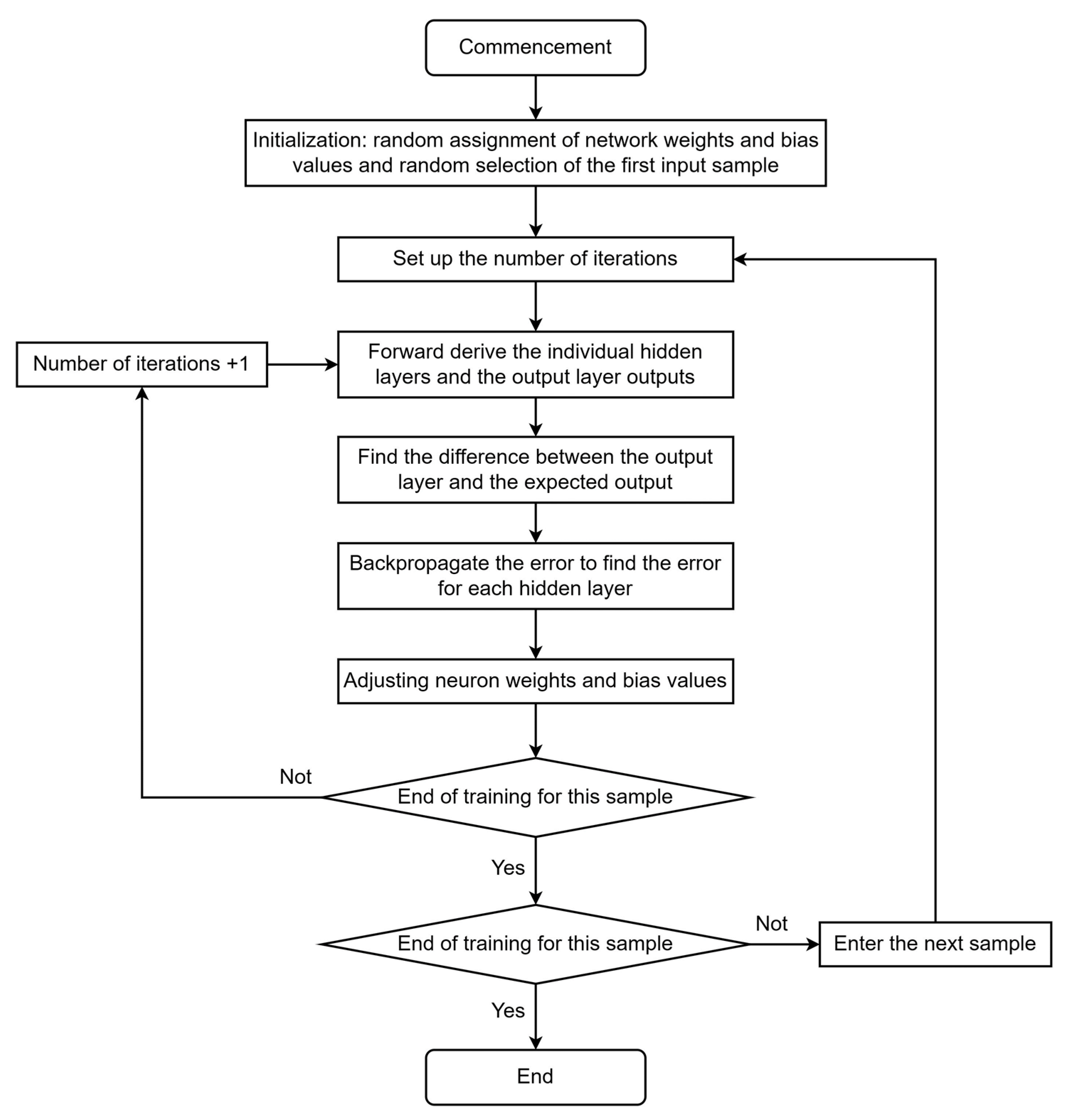
The Bayesian-Regularized Back Propagation Neural Network (BRBPNN) model, which will be referred to as the BPNN model later in this paper, has an algorithmic flow, as shown in Figure 3, which is divided into the following five main steps:
  • Initialize the network weights and bias values.
In order to ensure randomness during training, the network weights are different between different neurons, and w i ( 1 , 1 ) is generally selected. At the same time, each neuron is randomly set a bias value, which can be regarded as their own weights.
2.
Perform forward propagation.
A training sample is randomly selected, and the output of each neuron is obtained by linear combination of the inputs. In neural networks, we define:
  • w i , j ( n ) as the weight between the ith neuron of Layer (n) and the jth neuron of Layer (n + 1).
  • b i ( n ) as the bias term of the ith neuron of Layer (n + 1).
  • s j ( n ) as the input value of the jth neuron of Layer (n + 1).
  • θ ( s j ( n ) ) as the output of the jth neuron of Layer (n + 1) after the activation function.
With training, you can obtain:
s j ( n ) = i w i , j ( 1 ) x i + b j ( n )
The output h w , b ( x ) can be expressed as follows:
h w , b ( x ) = θ j w j , k ( n + 1 ) θ ( s j ( n ) ) + b k ( n + 1 )
3.
Calculate the error and back propagate.
The network weights and bias values in the first iteration are randomly selected; thus, there must be an error between the output value and the true value. Needless to say, the smaller the error, the better the prediction effect, so we need to reduce this error. The minimum mean square error (MMSE) is usually used to describe the error size in the training of neural networks. The mean square error E d (MSE) is expressed as follows:
E d = 1 n i = 1 n e i 2 = 1 n i = 1 n ( x ¯ x i ) 2
where x i is the sample value and x ¯ is the sample expectation. Then, the gradient descent method is used to obtain the minimum mean square error; that is, the weight of each sample is changed in the negative direction of its gradient. From Equation (22), we can obtain:
s j ( n ) w i , j ( n ) = x i
Then, for the weight gradient between the input layer and the hidden layer, there is:
E d w i , j ( n ) = E d s j ( n ) s j ( n ) w i , j ( n ) = E d s j ( n ) x i
Based on the passing of output from layer to layer, you can obtain:
s k ( n + 1 ) = k w j , k ( n + 1 ) θ s j ( n ) + b k n + 1
Combining the above equation with Equation (26), we can obtain:
E d s j ( n ) = θ ( s j ( n ) ) k E d s k ( n + 1 ) w j , k ( n + 1 )
Letting δ j ( n ) = E d / s j ( n ) and then simplifying the above equation and Equation (24) simultaneously, we can obtain:
δ j ( n ) = θ ( s j ( n ) ) k δ k ( n + 1 ) w j , k ( n + 1 )
δ k ( n + 1 ) = e k θ ( s k ( n + 1 ) )
From the above equation, it is easy to see that the core function to realize the backpropagation of the error is e k . In the process of back propagation, the output layer is re-used as the input layer, with e k as the input, through the activation function θ ( s k ( n + 1 ) ) . The reverse output δ k ( n + 1 ) of the output layer is obtained, and then it is combined with the weight w j , k ( n + 1 ) through the activation function θ ( s j ( n ) ) to obtain the reverse output δ j ( n ) of the hidden layer. At this point, the weight gradient shown in Equation (26) can be calculated.
4.
Updating the network weights.
Based on the weight gradient calculated above, the weights can be readjusted, which can be expressed as:
w i , j ( n ) t + 1 = w i , j ( n ) t ζ E d w i , j ( n )
where t is the number of iterations and ζ is the regulation rate.
5.
Determine if training is over.
For each sample, when the output value and the true value are less than the set maximum allowable error or the number of iterations reaches the maximum, the training ends and we return to step 2 to start the training for the next sample.
During the training of neural networks, overfitting often occurs due to the pursuit of a higher degree of fitting. In order to ensure a high degree of model fitting and to prevent overfitting, Bayesian regularization is often used in machine learning. Define the training performance function as F, which can be expressed as:
F = a E w + b E d
E w = 1 m m w i 2
where E w is the mean square error of the network weights, m is the number of network weights, and a and b are the regularization coefficients of the objective function F, which determines the training objective of the neural network. If b a , then the training is more inclined to improve the generalization ability of the neural network, but it will lead to a larger training error and underfitting; if b a , then the training is more inclined to reduce the training error of the network and cause overfitting. Thus, the values of a and b will directly affect the training results of the neural network.
Combined with Bayesian probability theory, the maximum a posteriori probability method is used to solve for the values of a and b in the case where the network weights obey a Gaussian distribution for the prior probability, which can be obtained via:
a = m n 2 E d
b = η 2 E w
where η is the number of effective weights of the neural network. It can be expressed as:
η = m 2 a t r H 1
where H is the Hessian matrix of the objective function F, which can in turn be expressed as:
H = a 2 E d + b 2 E w
Through Bayesian regularization, the program can adaptively adjust the values of a and b to effectively control the complexity of the neural network while ensuring that the training error of the neural network is as small as possible so as to optimize the fitting results.

2.5. Technical Route to Machine-Learning-Based FT-LB Coupled Modeling

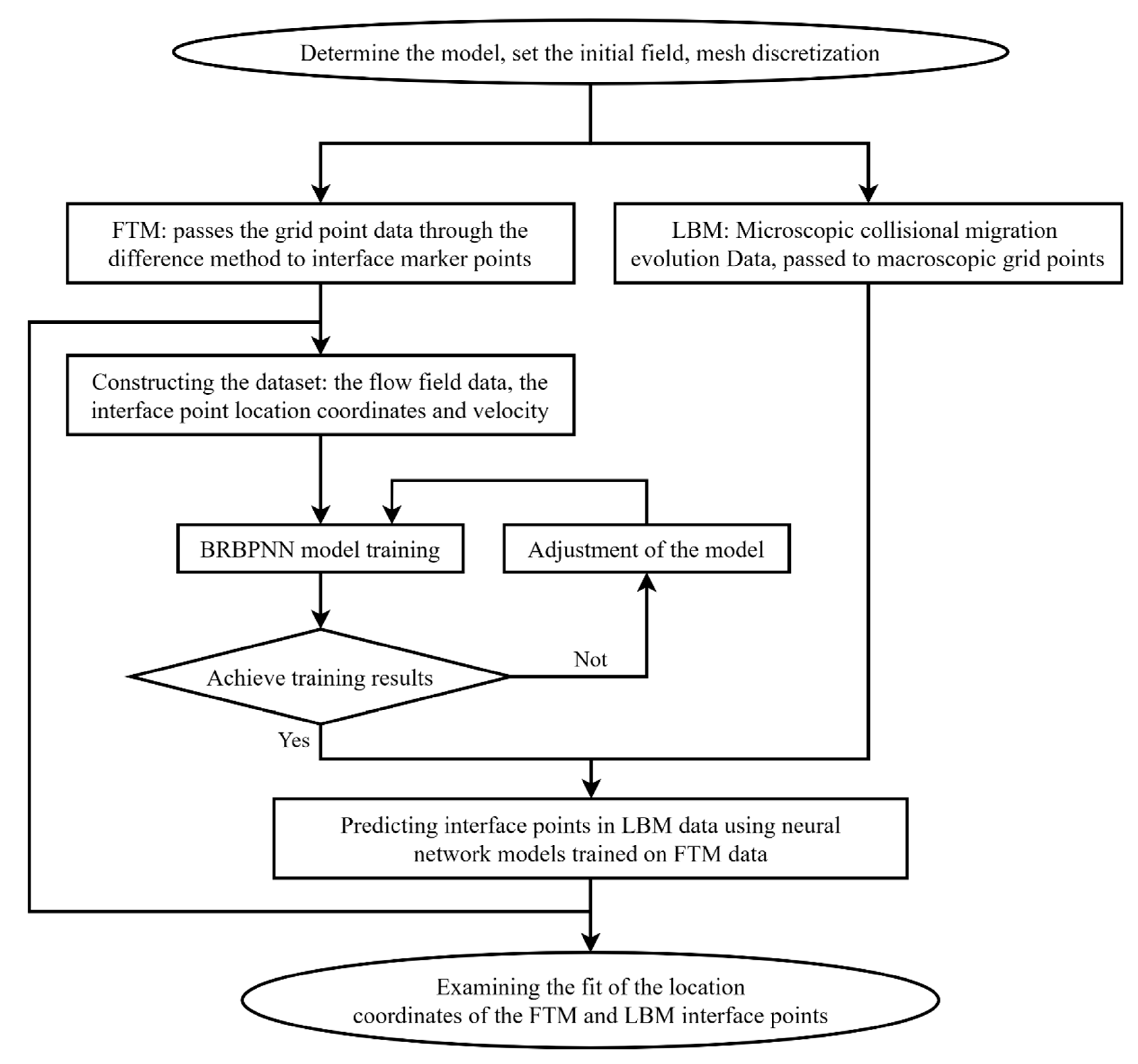
Figure 4 shows the technical flowchart of the FT-LB coupled model based on machine learning.
  • By using the FTM to simulate the motion process of single bubble ascent, the flow field information updated with time is obtained, and the position coordinates of each interface point, the position coordinates of each grid point, and the velocity corresponding to them are recorded, which are used to construct the input and output sets of the machine learning neural network.
  • In the current paper, the BRBPNN model is used to train the neural network for single bubble ascent, with the velocity field information of the basin as the input set of the neural network port and the interface marking point positions as the output set of the neural network port. The purpose of this is to construct the dataset and the test set, to study the optimal optimization and screening of the dataset, and then to study the optimization of the parameters of the neural network model in order to achieve the best training effect.
  • The upward motion process of a single bubble is simulated by using the LBM to obtain its flow field information, the velocity at the maximum density gradient in the basin is taken as the input to the trained neural network model, the predicted interface marking points in the Eulerian mesh of the LBM are output and compared with the interface marking points simulated by the FTM, and then the algorithms are verified in terms of their stability, accuracy, efficiency of the solution, and adaptability of the physical model. The FT-LB coupled computational model is then improved.

3. Modeling and Discussion

3.1. Front-Tracking Method Modeling

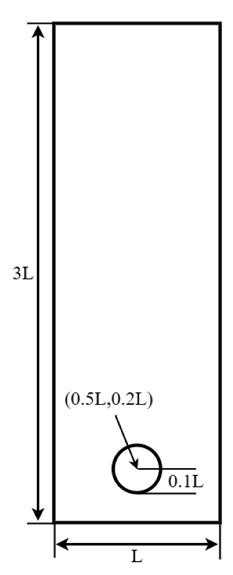
Since droplet rises are very common in fluid dynamics, in this paper, we chose to take a vacuole rise as the object of study. Figure 5 shows the diagram of the drainage basin used in the study of a single vacuole rise in the present paper. In the FTM simulation, the flow channel area is calculated as a rectangular area, and filled with a liquid of density ρ 1 and dynamic viscosity μ 1 , and the width and length of the domain are 1 L and 3 L, respectively. A grid of 100 in the x direction and 300 in the y direction is established on the basin, so the dimensionless grid length is 0.01 L. At the initial time, a circular vacuole with a diameter of 0.1 L, density ρ 2 and dynamic viscosity μ 2 is released at a certain position (0.5 L, 0.2 L). The surface tension coefficient is σ , the gravitational acceleration is g, and the boundary is a no-slip boundary. In the current paper, the rise time of the model was chosen to be 3 s and the time node was chosen to be 300 steps, so the dimensionless time step is 0.01. The control group is set to:
Case 1: ρ 1 / ρ 2 = 20, σ = 0.02, μ 1 / μ 2 = 10, g = −0.1.
In the process of the numerical simulation, for each time node, the velocity at 100 × 300 grid points is calculated. At the same time, 150 to 200 interface points are selected on the phase interface. The position coordinate ( x o u t , y o u t ) of each phase interface point, the position coordinate ( x , y ) of each grid point and the corresponding velocity ( u , v ) are recorded.

3.2. Grid-Independent Validation of the Front-Tracking Method Model

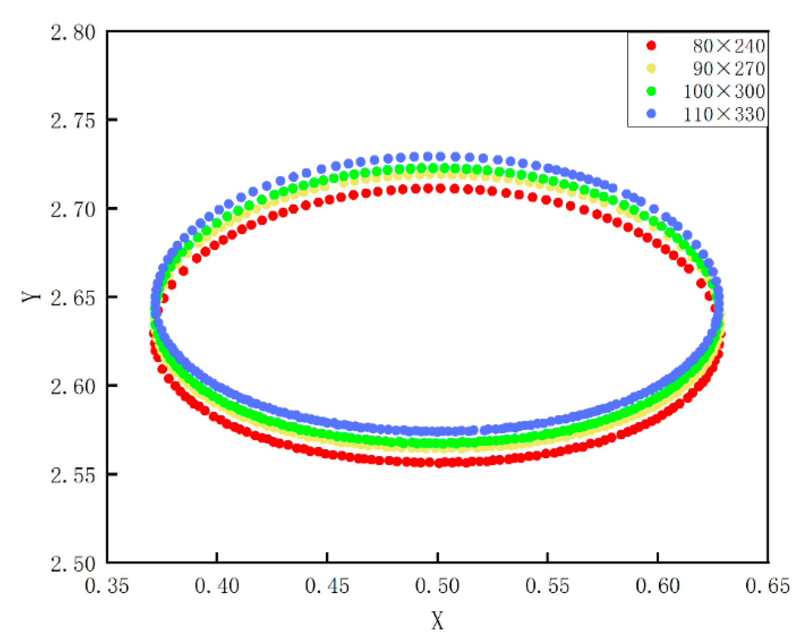
As shown in Figure 6, a uniform staggered grid is used for the calculation in the present paper. For the grid independence study, four different grids with grid points of 80 × 240, 90 × 270, 100 × 300 and 110 × 330 were used. When the dimensionless time is 300, comparing the rising position and morphological change of the final state of the vacuole rising process of these four grids, it can be seen that the difference between 80 × 240 and 110 × 330 grids is very large and the difference between 90 × 270 and 100 × 300 grids is very small, and this difference is within the allowable error range. Considering the accuracy and cost of the calculation, a grid of 100 × 300 was selected for the subsequent model.

3.3. Influence of the FTM-Based Surface Tension Coefficient and Kinetic Viscosity on the Rise of a Single Vacuole

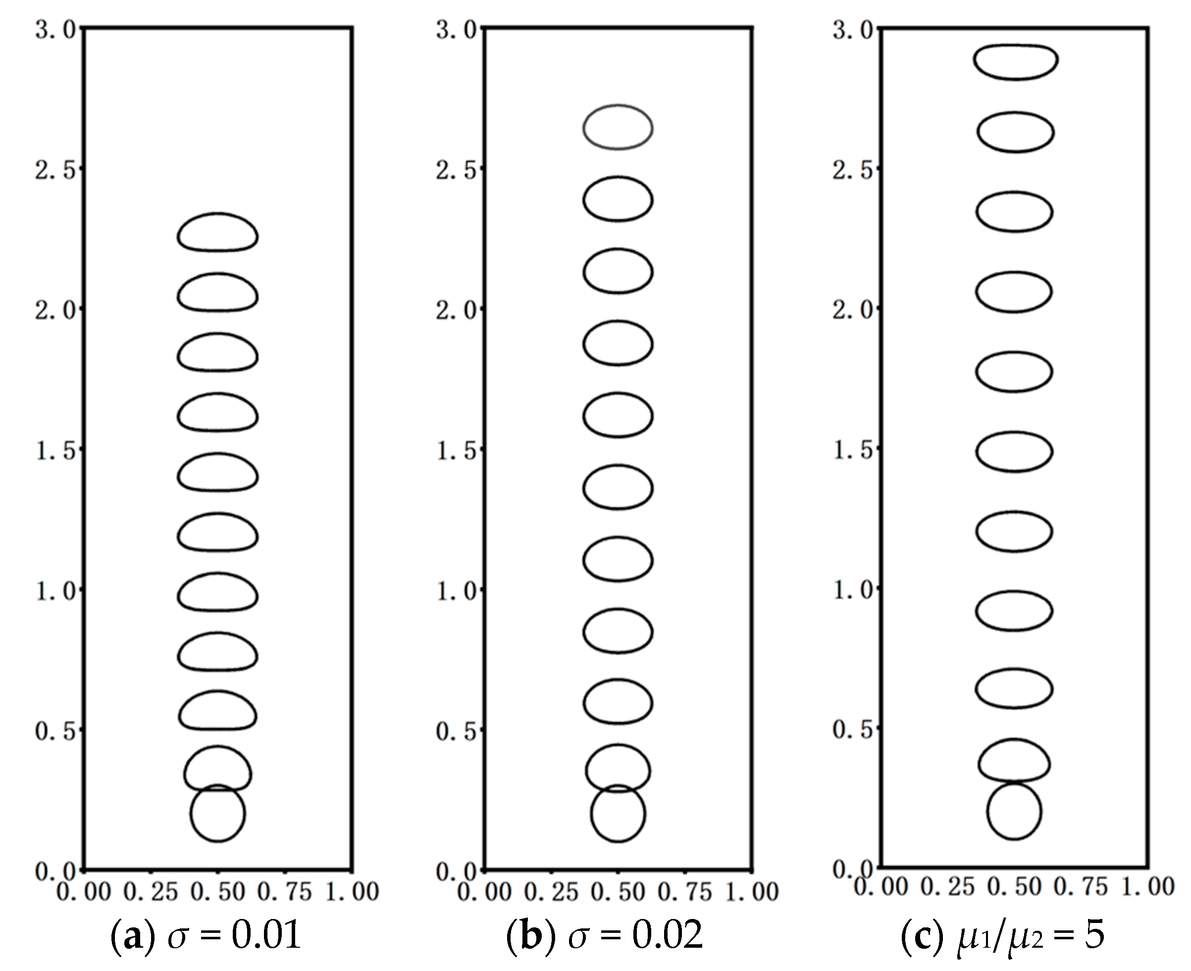
As shown in Figure 7, in the current paper, except for the control group, the surface tension coefficient is 0.01 and the dynamic viscosity ratio is 5. After FTM simulation calculations, in the process of vacuole rising, the surface tension of the vacuole decreases with the decrease in the surface tension coefficient. The easier the vacuole is to deform, the greater the deformation rate, which will increase the surface area accordingly. Under the combined action of gravity and viscous forces, it can be evidently seen that the upper surface of the vacuole also fluctuates more than the lower surface. As the dynamic viscosity ratio decreases, the viscous action of the vacuole by the viscous force decreases, and its rising speed will increase accordingly. At this time, the pressure and surface tension of the vacuole are mostly unchanged, and the decrease in the viscous force will increase the velocity gradient of the phase interface, resulting in an increasing deformation rate of the vacuole and a flatter shape of the vacuole in the final state.

3.4. Neural Network Modeling

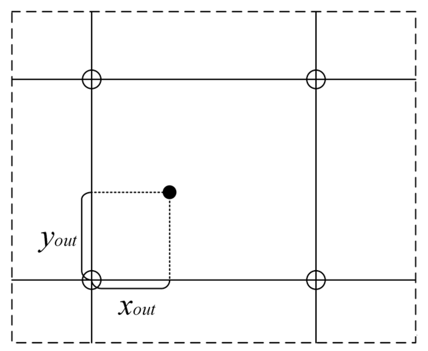
In the process of making the output set, in this paper, firstly, the interface point position coordinates (xout, yout) are taken as the output set, and the error is found to be large in the process of neural network training. In order to further improve the simulation accuracy and simulation rate of the BRBPNN model, the difference between the interface point position coordinates and the grid point position coordinates (dxout, dyout) is reselected as the output set, as shown in Figure 8.
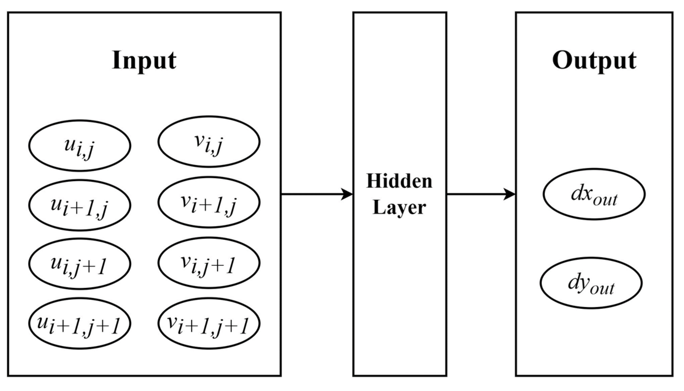
As shown in Figure 9, in the current paper, the difference (dxout, dyout) between the position coordinates of interface points and grid points is chosen as the output set of the BRBPNN model, and the velocity (u, v) of the four grid points closest to the phase interface point is chosen as the input set of the BRBPNN model, as shown in Figure 10.
As shown in Figure 11, in the parameter selection of the neural network, two hidden layers were set in the current study; the first hidden layer is selected to use 50 neurons, and the second hidden layer is selected to use 10 neurons. The activation function of the hidden layer is selected as TANSIG, the activation function of the output layer is selected as PURELIN, and the TRAINBR function is selected when passing forward. The minimum mean square error is selected as the loss function, the gradient descent method is selected as the optimization method of the loss function, the learning rate is selected as 0.01, and the number of learning steps is set to 10,000.
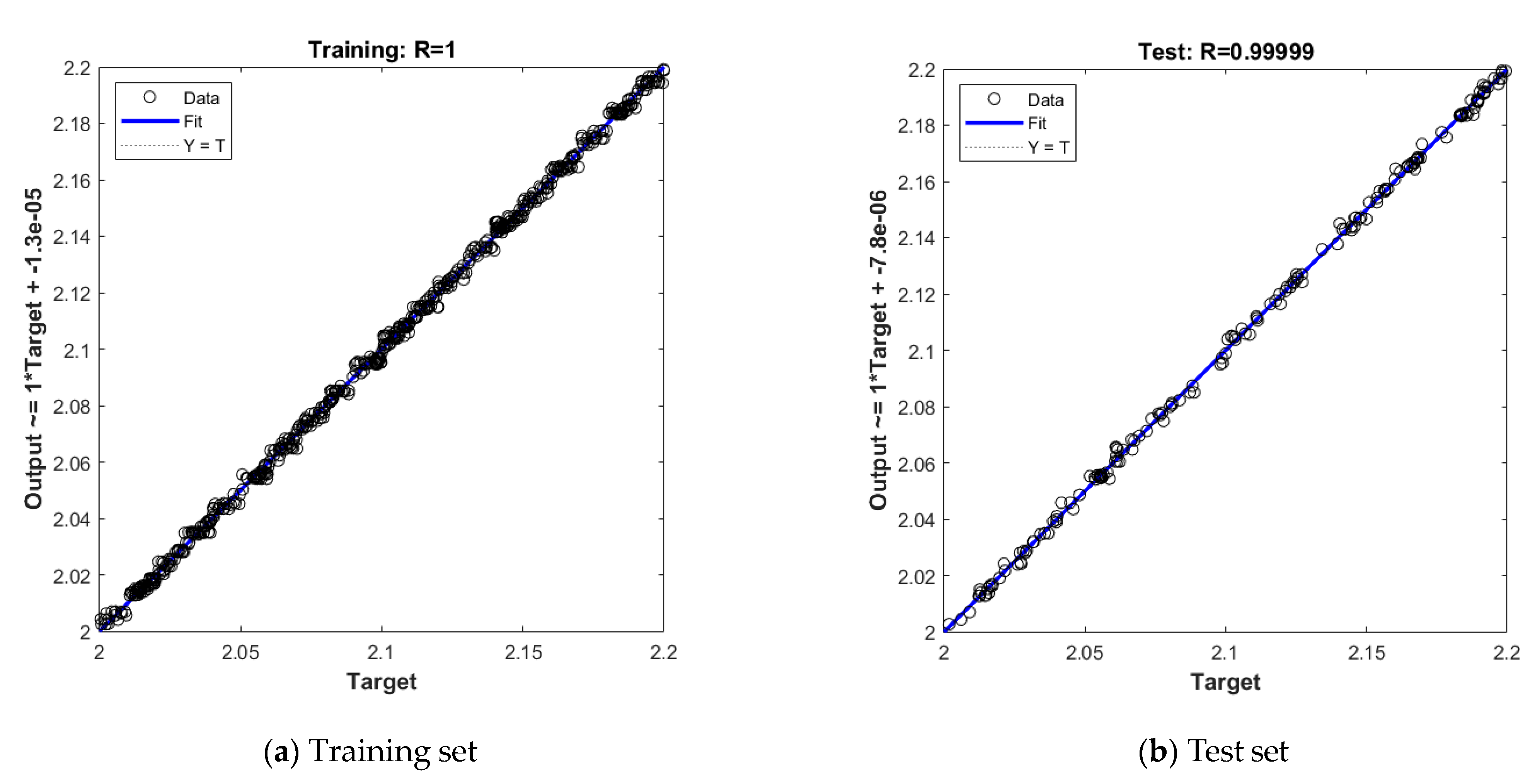
Figure 12 shows that the control variable method is used to take Case 1 as the control group, and the control group is taken as an example for illustration. Figure 12a shows the training results of the BRBPNN model in the training set, and the abscissa in the figure represents the x or y values of the predicted coordinates of the interface markers trained by the BRBPNN model with the speed of four grid points as input. The ordinate represents the dxout or dyout value of the coordinates of the interface markers in the FTM simulation, the data point represents the correspondence between the output value and the predicted value, the blue fit line represents the fitting line between the output value and the predicted value, and the Y = T line represents the fitting line when the fitting degree is the highest. It is easy to see that in order to achieve a better fitting effect, the fit line should coincide with the Y = T line to the greatest extent. In Figure 12a, the fit line has an angle of 45° with the coordinate axis, even covering the Y = T line, indicating that the training effect of the BRBPNN model is very good. On the other hand, the fitting degree coefficient R is obtained by calculating the mean square error of the output value and the predicted value. The higher the fitting degree, the closer the R value is to 1. The R value in Figure 12a is equal to 1, which further illustrates the accuracy of the BRBPNN model.
Figure 12b represents the training results of the BRBPNN model in the test set. The horizontal coordinate in the figure represents the x or y value of the predicted coordinates of the interface marker points obtained by the trained BRBPNN model with the speed of the four grid points as input; the vertical coordinate represents the dxout or dyout value of the coordinates of interface marker points in FTM simulations. The fit line overlaps with the Y = T line to a high degree. The R value is also 0.99999, indicating that the prediction performance of the trained BRBPNN model is very good and the feasibility meets the requirements.

3.5. Training Results of the BRBPNN Model with Different Surface Tension Coefficients and Dynamic Viscosity Ratios

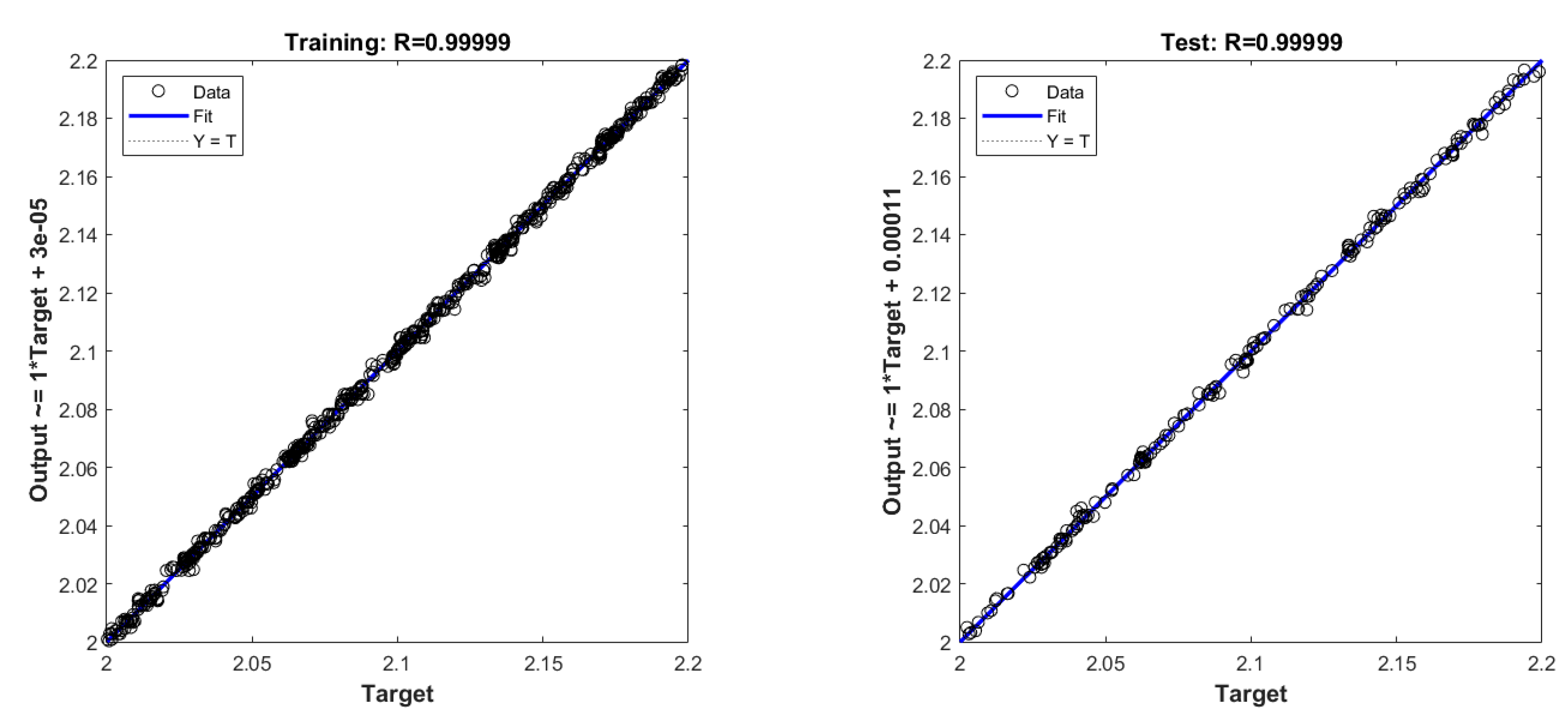
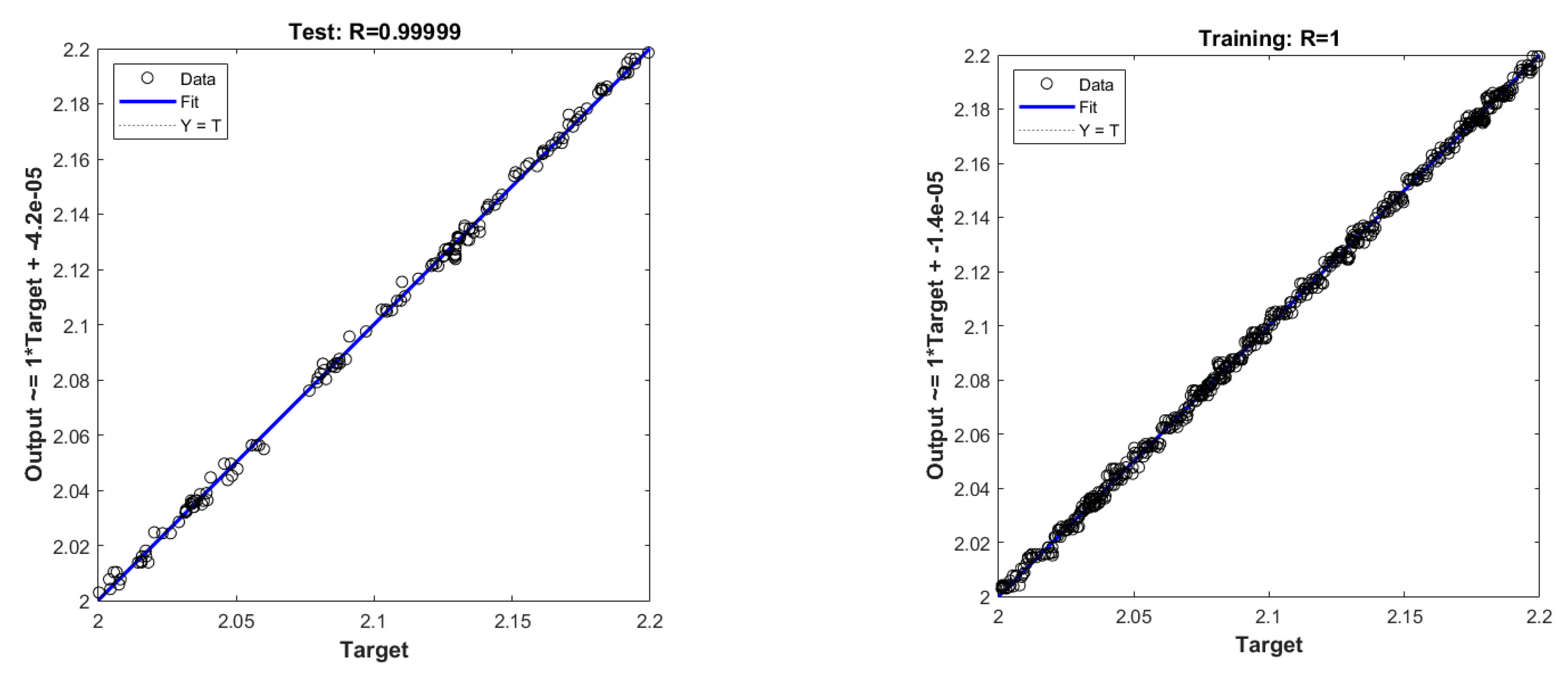
The training results of the BRBPNN model for each initial condition by varying the surface tension coefficient to 0.01 and by varying the kinetic viscosity ratio to 5 for both working conditions are shown in Figure 13 and Figure 14.
As shown in Figure 13 and Figure 14, by changing the surface tension coefficient, the fit line of dynamic viscosity has a high degree of coincidence with the Y = T line compared with the predicted value (x, y) and output value (dxout, dyout) of the test set and training set under the initial conditions, and the fitting degree coefficient R ∈ [0.99999, 1] indicates that the fitting effect is very good. The accuracy and feasibility of the BRBPNN model meet the requirements, and there are no underfitting or overfitting phenomena. The neural network training was successful, and interface point prediction using LBM numerical simulations can be continued in the next step.

3.6. Simulation Results of the Multi-Relaxation Lattice Boltzmann Pseudopotential Model

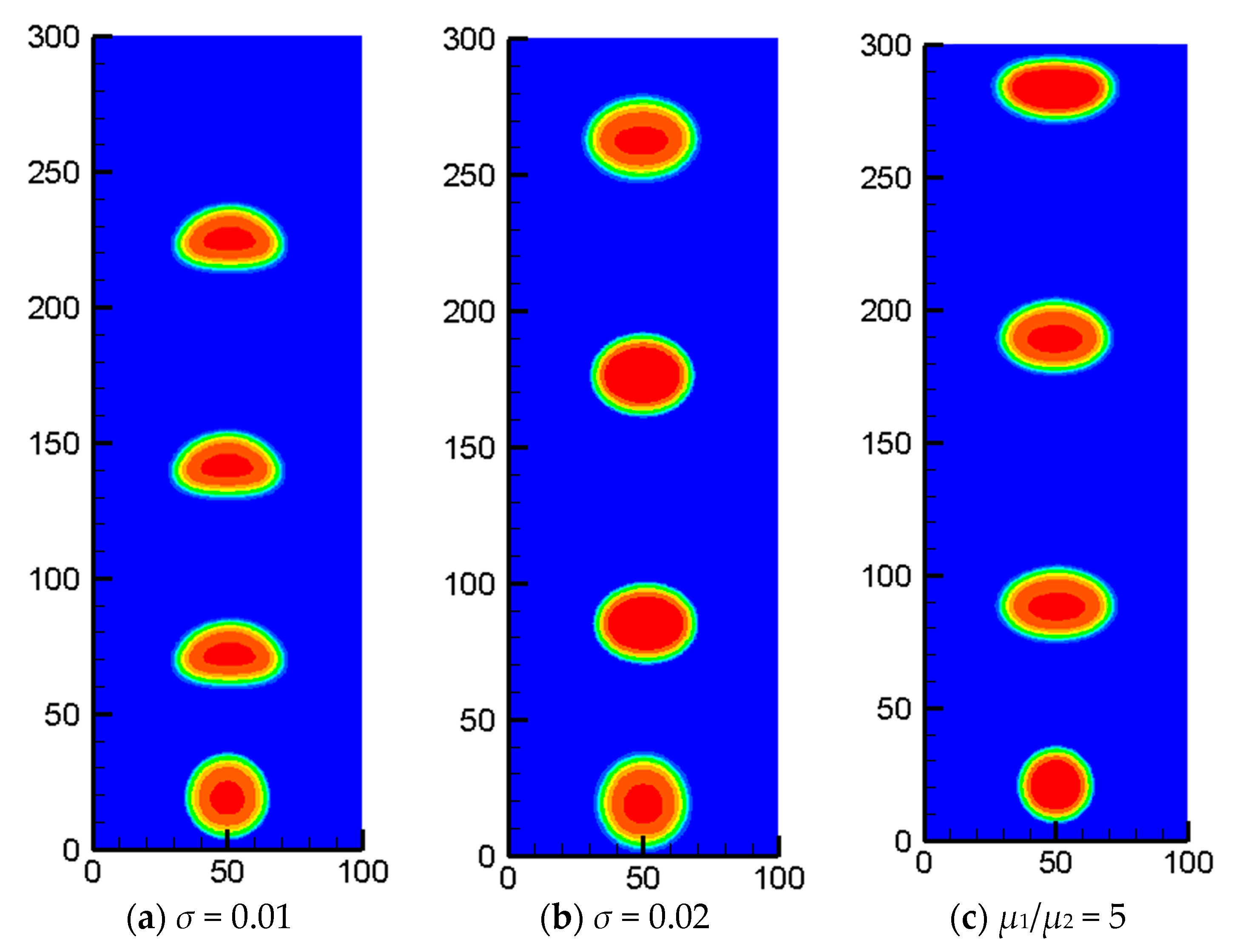
Figure 15 shows the density field distribution cloud map of the basin under various initial conditions through the simulation calculation of the multi-relaxation lattice Boltzmann pseudo-potential model. With the increase in the surface tension coefficient, the deformation rate of the vacuole also gradually decreases and the rising speed shows a gradual decreasing trend. With the increase in the dynamic viscosity ratio, the deformation rate of the vacuole also gradually decreases and the rising speed shows a gradual decreasing trend, which was consistent with the movement law of a single vacuole rising with a changing surface tension coefficient in FTM simulations.

3.7. Lattice Boltzmann Method Model Interface Point Prediction

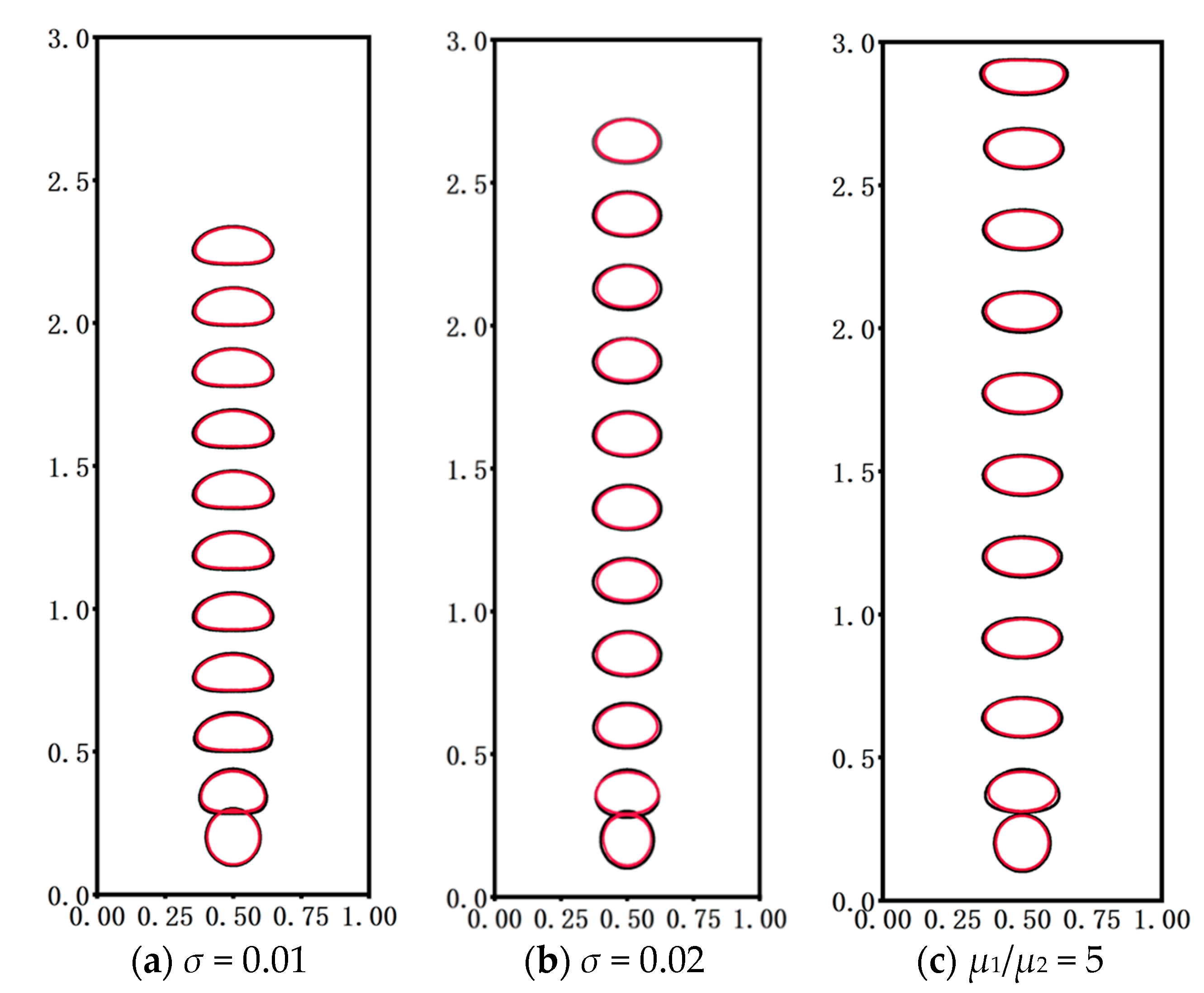
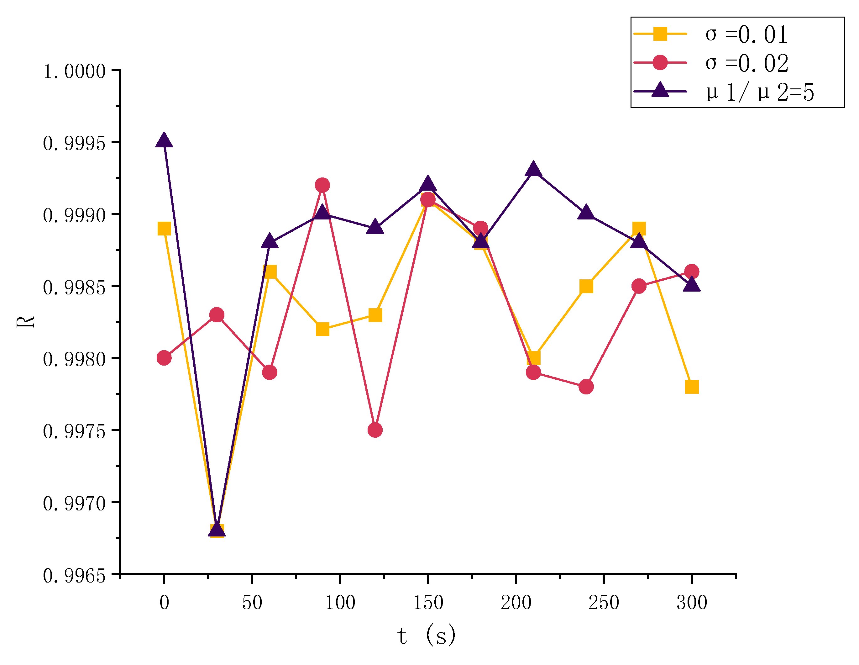
As shown in Figure 16, the trained BRBPNN neural network was used to predict the interface position of the LBM flow field, and the interface point position simulated by the FTM model is compared and verified. Under the condition of changing the surface tension coefficient and dynamic viscosity ratio, the predicted interface of the LBM is in good agreement with that of the FTM. As shown in Figure 17, its fitting degree coefficient R ∈ [0.9965, 1] once again proves that the fitting effect is very good.

4. Conclusions

The current paper innovatively proposes a coupled numerical algorithm based on machine learning to achieve an FT-LB method for accurate interface modeling and dynamic process simulations of fluid flow phases at the mesoscopic scale. Taking a single vacuole rising as the model, the following conclusions were reached:
(1)
By inputting the LBM’s grid point velocities into the trained neural network, the location of the phase interface is accurately labeled and the problem of ambiguous descriptions of the phase interface in LBM simulations is successfully solved.
(2)
The accuracy and feasibility of the BRBPNN model meet the requirements of the FT-LB coupling model. The FT-LB coupling model based on BRBPNN machine learning is constructed, and its feasibility regarding adjustability and accuracy is verified by simulations of different working conditions.
(3)
Considering a more complex multiphase flow process, three-dimensional physical models can be considered in future studies. It is expected that future research will delve further into the phenomenon of liquid structural damage and expand the scope of the study to cover more complex scenarios.

Author Contributions

Conceptualization, P.L., Y.Z. and J.L.; Methodology, P.L., Y.Z., J.L. and Y.T.; Formal analysis, P.L., H.Z., Z.K., Y.Z., J.L. and Y.T.; Investigation, S.Z.; Resources, P.L., Y.Z. and J.L.; Data curation, H.Z., Z.K., S.Z. and Y.Z.; Writing—original draft, H.Z.; Writing—review & editing, H.Z., Z.K. and Y.T.; Visualization, Z.K. and S.Z.; Project administration, Y.T.; Funding acquisition, P.L. and J.L. All authors have read and agreed to the published version of the manuscript.

Funding

The work was supported by the National Natural Science Foundation of China (No. 52166009).

Data Availability Statement

No new data were created or analyzed in this study. Data sharing is not applicable to this article.

Conflicts of Interest

The authors declare no conflict of interest.

Nomenclature

aAcceleration of the Particle (m/s2) x ¯ Sample Expectation
bBias Term(x, y)Cartesian Coordinate Components
cLattice Velocity (m/s)(u, v)Velocity Component along x,y Direction
CMotion Velocity of the Particle (m/s)Greek Symbols
eDiscrete Velocity (m/s)γRelaxation Time
EdMean Square ErrorδtParticle Movement Time (s)
FInteraction ForceδReverse Output
fParticle Distribution FunctionζRegulation Rate
f e q Equilibrium Distribution FunctionθActivation Function
h(x)Output ResultμViscosity
gGravitational Acceleration (m/s2) ρ Density (kg/m3)
GStrength of Interaction σ Surface Tension Coefficient
LConstant ψ Interaction Potential
pPressure (pa)ωWeight Factor of Interaction
rPosition Coordinate of the ParticleSuberscripts
RFitting Degree CoefficienthStep Size
sInput ValueiNeuron Code
tTime (s)jNeuron Code
Δ t Time StepkNeuron Code
uVelocity Vector (m/s)nCertain Moment
u*Temporary Velocity (m/s)n + 1Next Moment of Moment
wWeighting Factor Constant α Cartesian Coordinate Components
Δ x Space StepoutOutput Item
xiSample ValuetNumber of Iterations

References

  1. Yuan, Z.; Wu, R.; Wu, X. Numerical simulations of multi-hop jumping on Superhydrophobic Surfaces. Int. J. Heat Mass Transf. 2019, 135, 345–353. [Google Scholar] [CrossRef]
  2. Lin, S.; Lu, J.; Tryggvason, G.; Zhang, Y. The effect of fluid shear on oscillating bubbly flows. Phys. Fluids 2019, 31, 042110. [Google Scholar] [CrossRef]
  3. Lu, M.; Lu, J.; Zhang, Y.; Gretar, T. Effect of electrostatic forces on the distribution of drops in turbulent channel flows. Phys. Fluids 2019, 31, 105104. [Google Scholar] [CrossRef]
  4. Tryggvason, G.; Bunner, B.; Esmaeeli, A.; Juric, D.; Al-Rawahi, N.; Tauber, W.; Han, J.; Nas, S.; Jan, Y.J. A Front-Tracking Method for the Computations of Multiphase Flow. J. Comput. Phys. 2001, 169, 708–759. [Google Scholar] [CrossRef]
  5. Unverdi, S.O.; Tryggvason, G. A Front-Tracking Method for Viscous, Incompressible, Multi-Fluid Flows. J. Comput. Phys. 1992, 100, 25–37. [Google Scholar] [CrossRef]
  6. Li, W.; Lu, J.; Tryggvason, G.; Zhang, Y. Numerical study of droplet motion on discontinuous wetting gradient surface with rough strip. Phys. Fluids 2021, 33, 012111. [Google Scholar] [CrossRef]
  7. Lu, J.; Fernández, A.; Tryggvason, G. The Effect of Bubbles on The Wall Drag in A Turbulent Channel Flow. Phys. Fluids 2005, 17, 095102–095113. [Google Scholar] [CrossRef]
  8. Min, L.; Jiacai, L.; Ying, Z.; Gretar, T. Numerical Study of Thermocapillary Migration of a Bubble in A Channel with An Obstruction. Phys. Fluids 2019, 31, 062101. [Google Scholar]
  9. Juric, D.; Tryggvason, G. Computations of Boiling Flows. Int. J. Multiph. Flow 1998, 24, 387–410. [Google Scholar] [CrossRef]
  10. Li, Q.; Luo, K.H.; Kang, Q.J.; He, Y.L.; Chen, Q.; Liu, Q. Lattice Boltzmann Methods for Multiphase Flow and Phase-Change Heat Transfer. Physics 2015, 52, 62–105. [Google Scholar] [CrossRef]
  11. Zhaoli, G.; Chuguang, Z. Principles and Applications of The Lattice Boltzmann Method; Science Press: Beijing, China, 2009. [Google Scholar]
  12. Yaling, H.; Qing, L.; Yong, W. Theory and Application of Lattice Boltzmann Method; China Education Publishing Media Group: Beijing, China; Higher Education Press: Beijing, China, 2023. [Google Scholar]
  13. Wandong, Z. Theoretical and Applied Study of The Pseudopotential Multiphase Lattice Boltzmann Model. Ph.D. Thesis, Nanchang University, Nanchang, China.
  14. Shan, X.; Chen, H. Lattice Boltzmann Model for Simulating Flows with Multiple Phases and Components. Phys. Rev. E 1993, 47, 1815–1819. [Google Scholar] [CrossRef] [PubMed]
  15. Kupershtokh, A.L.; Karpov, D.I.; Medvedev, D.A. Stochastic Models of Partial Discharge Activity in Solid and Liquid Dielectrics. Sci. Meas. Technol. IET 2007, 1, 303–311. [Google Scholar] [CrossRef]
  16. Guo, Z.L.; Zhao, T.S. Discrete Velocity and Lattice Boltzmann Models for Binary Mixtures of Nonideal Fluids. Phys. Review. E Stat. Nonlinear Soft Matter Phys. 2003, 68, 035302. [Google Scholar] [CrossRef] [PubMed]
  17. Li, Q.; Luo, K.H.; Li, X.J. Forcing Scheme in Pseudopotential Lattice Boltzmann Model for Multiphase Flows. Phys. Rev. E Stat. Nonlinear Soft Matter Phys. 2012, 86, 016709. [Google Scholar] [CrossRef]
  18. Kupershtokh, A.L.; Medvedev, D.A.; Karpov, D.I. On Equations of State in A Lattice Boltzmann Method. Comput. Math. Appl. 2009, 58, 965–974. [Google Scholar] [CrossRef]
  19. Zhao, Y.; Liang-Shih, F. Multirelaxation-Time Interaction-Potential-Based Lattice Boltzmann Model for Two-Phase Flow. Phys. Rev. E. Stat. Nonlinear Soft Matter Phys. 2010, 82, 046708. [Google Scholar]
  20. McCracken, M.E.; Abraham, J. Multiple-Relaxation-Time Lattice-Boltzmann Model for Multiphase Flow. Phys. Rev. E 2005, 71, 036701. [Google Scholar] [CrossRef] [PubMed]
  21. Lallemand, P.; Luo, L.-S.; Peng, Y. A Lattice Boltzmann Front-Tracking Method for Interface Dynamics with Surface Tension in Two Dimensions. J. Comput. Phys. 2008, 226, 1367–1384. [Google Scholar] [CrossRef]
  22. Sui, Y.; Low, H.T.; Chew, Y.T.; Roy, P. A Front-Tracking Lattice Boltzmann Method to Study Flow-Induced Deformation of Three-Dimensional Capsules. Comput. Fluids 2010, 39, 499–511. [Google Scholar] [CrossRef]
  23. Haiqiong, X.; Zhong, Z.; Liangqi, Z. Three-Dimensional Multi-Relaxation-Time Lattice Boltzmann Front-Tracking Method for Two-Phase Flow. Chin. Phys. B 2016, 25, 667–672. [Google Scholar]
  24. Yuan, Z.; Gao, S.; Hu, Z.; Dai, L.; Hou, H.; Chu, F.; Wu, X. Ultimate jumping of coalesced droplets on superhydrophobic surfaces. J. Colloid Interface Sci. 2020, 587, 429–436. [Google Scholar] [CrossRef] [PubMed]
  25. Yuan, Z.; Hou, H.; Dai, L.; Wu, X.; Tryggvason, G. Controlling the Jumping Angle of Coalescing Droplets Using Surface Structures. ACS Appl. Mater. Interfaces 2020, 12, 52221–52228. [Google Scholar] [CrossRef] [PubMed]
  26. Bishop, C.M.; James, G.D. Analysis of Multiphase Flows Using Dual-Energy Gamma Densitometry and Neural Networks. Nucl. Instrum. Methods Phys. Res. Sect. A-Accel. Spectrometers Detect. Assoc. Equip. 1993, 327, 580–593. [Google Scholar] [CrossRef]
  27. Milano, M.; Koumoutsakos, P. Neural Network Modeling for Near Wall Turbulent Flow. J. Comput. Phys. 2002, 182, 1–26. [Google Scholar] [CrossRef]
  28. Ma, X.; Wang, C.; Huang, B.; Wang, G. Application of Two-Branch Deep Neural Network to Predict Bubble Migration Near Elastic Boundaries. Phys. Fluids 2019, 31, 102003. [Google Scholar] [CrossRef]
  29. Han, R.; Wang, Y.; Zhang, Y.; Chen, G. A Novel Spatial-Temporal Prediction Method for Unsteady Wake Flows Based on Hybrid Deep Neural Network. Phys. Fluids 2019, 31, 127101. [Google Scholar] [CrossRef]
  30. Chen, R.; Jin, X.; Li, H. A machine learning based solver for pressure Poisson equations. Theor. Appl. Mech. Lett. 2022, 12, 100362. [Google Scholar] [CrossRef]
  31. Brenner, M.P.; Eldredge, J.D.; Freund, J.B. Perspective on machine learning for advancing fluid mechanics. Phys. Rev. Fluids 2019, 4, 100501. [Google Scholar] [CrossRef]
  32. Qian, Y.X.; Zhang, T. The Second Order Projection Method in Time for The Time-Dependent Natural Convection Problem. Appl. Math. 2016, 61, 299–315. [Google Scholar] [CrossRef]
  33. Bell, J.; Solomon, J.; Szymczak, W. A Second-Order Projection Method for The Incompressible Navier Stokes Equations on Quadrilateral Grids. In Proceedings of the 9th Computational Fluid Dynamics Conference, Buffalo, NY, USA, 13–15 June 1989. [Google Scholar]
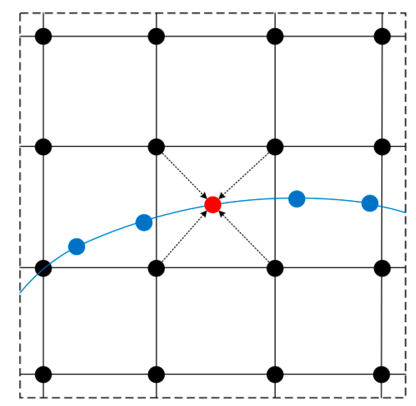
Figure 1. Schematic diagram of the difference between interface points and grid points.
Mathematics 12 00109 g001
Figure 2. Schematic of discrete velocities in the D2Q9 model.
Mathematics 12 00109 g002
Figure 3. BRBPNN model algorithm flow.
Mathematics 12 00109 g003
Figure 4. Flowchart of machine-learning-based FT-LB coupled modeling technique.
Mathematics 12 00109 g004
Figure 5. Schematic diagram of the watershed model.
Mathematics 12 00109 g005
Figure 6. Schematic of FTM simulation results for different meshes.
Mathematics 12 00109 g006
Figure 7. Plot of FTM simulation results for different surface tension coefficients and dynamic viscosity ratios.
Mathematics 12 00109 g007
Figure 8. Schematic diagram of the differential output.
Mathematics 12 00109 g008
Figure 9. Schematic of BRBPNN model inputs and outputs.
Mathematics 12 00109 g009
Figure 10. Schematic of grid point selection.
Mathematics 12 00109 g010
Figure 11. Schematic diagram of machine learning parameter settings.
Mathematics 12 00109 g011
Figure 12. BRBPNN model training results for control Case 1.
Mathematics 12 00109 g012
Figure 13. Training results of the BRBPNN model for changing σ to 0.01.
Mathematics 12 00109 g013
Figure 14. Training results of the BRBPNN model for changing μ1/μ2 to 5.
Mathematics 12 00109 g014
Figure 15. Cloud view of the density field of the simulated flow field with different surface tension coefficients and kinetic viscosity ratios of LBMs.
Mathematics 12 00109 g015
Figure 16. FT-LB couplings for different surface tension coefficients and dynamic viscosity ratios.
Mathematics 12 00109 g016
Figure 17. Plot of different surface tension coefficients and kinetic viscosity ratio fits.
Mathematics 12 00109 g017
Disclaimer/Publisher’s Note: The statements, opinions and data contained in all publications are solely those of the individual author(s) and contributor(s) and not of MDPI and/or the editor(s). MDPI and/or the editor(s) disclaim responsibility for any injury to people or property resulting from any ideas, methods, instructions or products referred to in the content.