Mathematical Solution of Temperature Field in Non-Hollow Frozen Soil Cylinder Formed by Annular Layout of Freezing Pipes

Abstract

With the wide application of the artificial ground freezing method in municipal underground engineering, the annular layout of freezing pipes is often adopted to form a frozen soil cylinder. However, there is still no analytical solution that can calculate the temperature distribution of frozen soil formed in this case. In this paper, a mathematical model of a steady-state temperature field of single-circle freezing is established, in which the inside of the freeze ring is completely frozen; that is, the temperature of all excavation sections is below the freezing point. Then, the analytical solution of temperature distribution is deduced through the complex variable method and potential superposition method. Comparison results of the analytical solution with those of the numerical simulation show that the analytical solution is precise enough. The temperature distribution of the main section and the intersection is approximately the same on the inner side, but the freezing effect of the main section is relatively better near the freezing pipes and outside the freeze ring. Besides, according to the derived analytical solution and common freezing parameters, a simplified formula to calculate the temperature field with enough accuracy was proposed, and the error can be controlled below 1‰. Finally, based on the simplified formula, a calculation method for frozen soil thickness and the average temperature is also given in this paper.

1. Introduction

Because of the stability in defending water and priority in safety and environmental protection, the artificial ground freezing method is now widely used in urban underground engineering, especially for excavation construction inside the water-rich soft ground. By arranging freezing pipes around the proposed underground space, a continuously closed frozen curtain is gradually formed in the stratum by artificial cooling technology, and then the subsequent excavation construction is carried out. Since the formed frozen soil curtain has good mechanical properties and the ability to isolate groundwater, it can give full play to its superiority in the groundwater-proof role and has been widely used in municipal underground projects [1,2], such as shield inlet and outlet the working shaft, tunnel contact channels, foundation pit support, etc.

For this method of formation reinforcement, unlike conventional grouting schemes, temperature field calculation is the basis of artificial ground freezing research, design, and construction. This is because all parameters, such as mechanical properties and strength index of frozen soil depend on the distribution of the frozen temperature field. Therefore, for different types of freezing works, accurate calculation of their freezing temperatures is an important guarantee for safe construction [3,4]. Numerous engineering practices and numerical calculations have shown that the temperature field of frozen soil is close to the steady-state temperature field at the later stage of artificial ground freezing. So, it is feasible to calculate the temperature field of artificial freezing projects using steady heat conduction, which is generally accepted by the academia and engineering sectors [5,6]. Compared with the experimental and numerical studies, the analytical solution can express the quantitative relationship between the temperature field and each influencing factor explicitly, and the physical meaning is clearer, so it is always an important content of the theoretical study of the artificial ground freezing method.

Based on the steady heat conduction theory, former Soviet scholars proposed several classical analytical solutions on the temperature field of artificial ground freezing. In 1954, TRUPAK, as the first one, proposed the method to calculate the temperature field of a frozen wall. Beginning with the research on single-piped freezing temperature, he derived the analytical solution of temperature field with single-row-piped freezing on the basis of a geometric relationship between freezing pipes and frozen soil columns [6]. BAKHOLDIN derived temperature field formulation of single-row-piped freezing and double-row-piped freezing, based on the theory of analogy between thermal and hydraulic problems [7]. In China, the research group from Tongji University improved these formulas and derived the analytical solution of different freezing schemes by means of superposition of potential function [8,9,10,11,12]. These previous works provide a very valuable reference for the calculation of the freezing temperature field.

However, due to the complexity and variability of design schemes and engineering geology in practical underground projects [13,14,15], the existing analytical solutions for temperature fields do not meet the needs of field applications. As far as the perimeter-closed freeze hole arrangement is concerned, the annular layout of freezing pipes is also often used in mining and municipal tunnel engineering, but the analytical solution of the temperature field can only calculate the hollow frozen soil column at present [16], and still cannot be solved for non-hollow frozen soil cylinder with negative temperatures in the full section during the late freezing period. Based on the potential function method, as well as the conformal mapping theory and the theory of analogy between thermal and hydraulic problems [17,18,19,20,21], this paper derives the mathematical solution of a steady-state temperature field in a frozen soil cylinder formed by single-circle freezing pipes, in order to grasp the temperature distribution of non-hollow frozen soil columns and prevent engineering accidents caused by insufficient frozen wall strength. First, we obtained the expression formula of potential with an eccentric well via potential function theory and mirror image method. On the basis of this formula, we then derive the formula of potential with a circular arrangement of wells using the complex function method. Next, considering the similarity between thermal and hydraulic problems, we derive the solution of the steady-state temperature field of annular arranged freezing pipes. Finally, we adopted the finite element method to prove the reliability of the obtained solution and proposed a calculation method for the thickness and average temperature of frozen soil in order to provide a reference for practical freezing works.

2. Potential Function in Hydrodynamics

Potential is a concept of energy in energy such as gravitational potential and electrostatic potential. The potential often represents a determined value, the gradient of which forms a force field. Potential field is often described with Laplace’s equation, whose solution is called potential function [22].

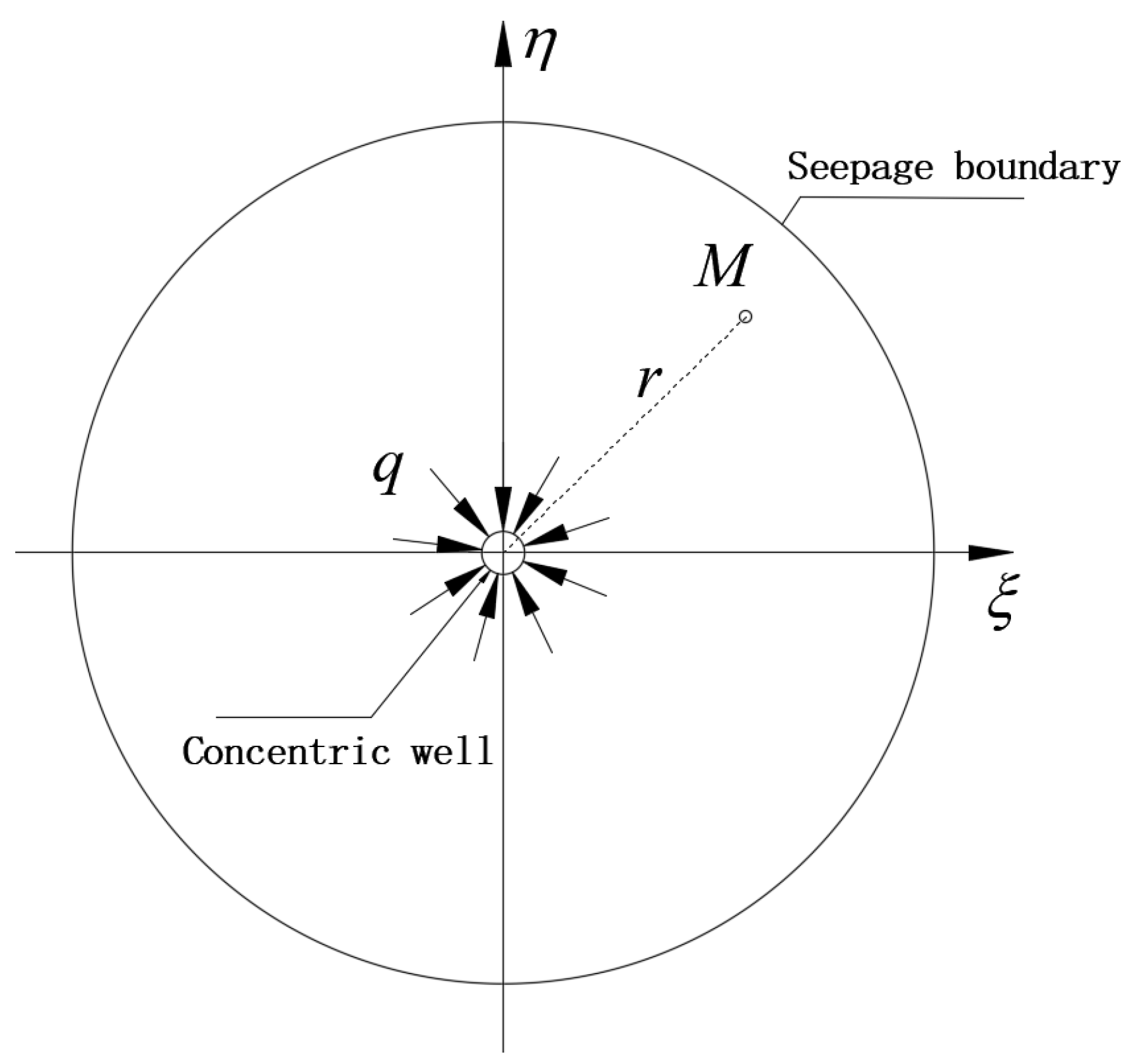
2.1. Potential Function of a Concentric Well

When only one well exists in an infinite formation with a circular seepage boundary, a plane right angle coordinate system is established with the well center as the coordinate origin, and the model is shown in Figure 1.

According to the research conclusions in the field of oil and gas extraction [23], the expression of hydraulic potential for any certain point M in stratum can be written as follows:

$${\Phi }_{\mathrm{M}}=\frac{q}{2\pi }\ln r+C$$

(1)

where q represents the flow volume per unit time; r represents the distance of the point to the well center; C is an integral constant determined by seepage boundary conditions.

2.2. Potential Function of an Eccentric Well

When this well is not at the origin of the coordinates, but there is an eccentric distance d₁, without loss of generality, it is assumed that the well is on the horizontal axis ξ. The geometric model is established as shown in Figure 2.

According to the mirror image method, mirroring the eccentric inlet well conjugally with equal strength and opposite sign by the circular seepage boundary, we can obtain a mirror outlet well with the same flow volume q. So, the problem is converted to the solving of the condition that in infinite stratum, there exists an inlet well q and an outlet well −q. With the rules of mirror reflection, the polar radius of the mirror well center is d₂ = ds²/d₁. Where d₁ is the polar radius of the center of inlet well q, d_s is the radius of the seepage boundary. Therefore, for this condition of circular stratum with an eccentric well, expression of potential at any random point M is as follows based on the principle of potential superposition [24]:

$${\Phi }_{\mathrm{M}}=\frac{q}{2\pi }\ln r_1-\frac{q}{2\pi }\ln r_2+C=\frac{q}{2\pi }\ln \frac{r_1}{r_2}+C$$

(2)

where q is the flow volume of the eccentric well; C is an integral constant.

According to the geometric relations in Figure 2 there are the following:

$$r_1=\sqrt{r^2+d_1{}^2-2r{d}_1\cos \theta }$$

(3)

$$r_2=\sqrt{r^2+d_2{}^2-2r{d}_2\cos \theta }=\sqrt{r^2+{(d_s{}^2/d_1)}^2-2r(d_s{}^2/d_1)\cos \theta }$$

(4)

where r is the polar radius of point M; θ is the polar angle of M.

Substituting (3), (4) into (2), potential at M can be expressed as follows:

$$\begin{array}{ll}{\Phi }_{\mathrm{M}}& =\frac{q}{2\mathsf{\pi }}\ln \frac{r_1}{r_2}+C\\ & =\frac{q}{4\mathsf{\pi }}\ln \frac{r^2+d_1{}^2-2r{d}_1\cos \theta }{r^2+{(d_s{}^2/d_1)}^2-2r(d_s{}^2/d_1)\cos \theta }+\mathrm{C}\\ & =\frac{q}{4\mathsf{\pi }}\ln \frac{\frac{r}{d_1}+\frac{d_1}{r}-2\cos \theta }{\frac{r{d}_1}{d_s{}^2}+\frac{d_s{}^2}{r{d}_1}-2\cos \theta }+{\Phi }_{\mathrm{s}}\end{array}$$

(5)

where Φ_s represents the potential on the seepage boundary, it can be expressed as follows [25]:

$${\mathsf{\Phi }}_s=\frac{q}{2\mathsf{\pi }}\ln \frac{d_1}{d_s}+C$$

(6)

When the point M is located at the border of the inlet well, the potential Φ_M should be equal to Φ_w, which represents the potential at the border of the well. Substitute Φ_M = Φ_W into (5), the flow volume of the eccentric well (q) can be calculated as follows:

$$q=\frac{4\mathsf{\pi }({\Phi }_W-{\Phi }_s)}{\ln \frac{\frac{d_1+d_w}{d_1}+\frac{d_1}{d_1+d_w}-2}{\frac{(d_1+d_w)d_1}{d_s{}^2}+\frac{d_s{}^2}{(d_1+d_w)d_1}-2}}=\frac{2\mathsf{\pi }({\Phi }_s-{\Phi }_W)}{\ln \left[-\frac{d_1}{d_s}+\frac{d_s}{d_w}-\frac{d_1{}^2}{d_w{d}_s}\right]}$$

(7)

where d_w is the radius of the eccentric well.

3. Temperature Field Solution with Annular Layout of Freezing Pipes

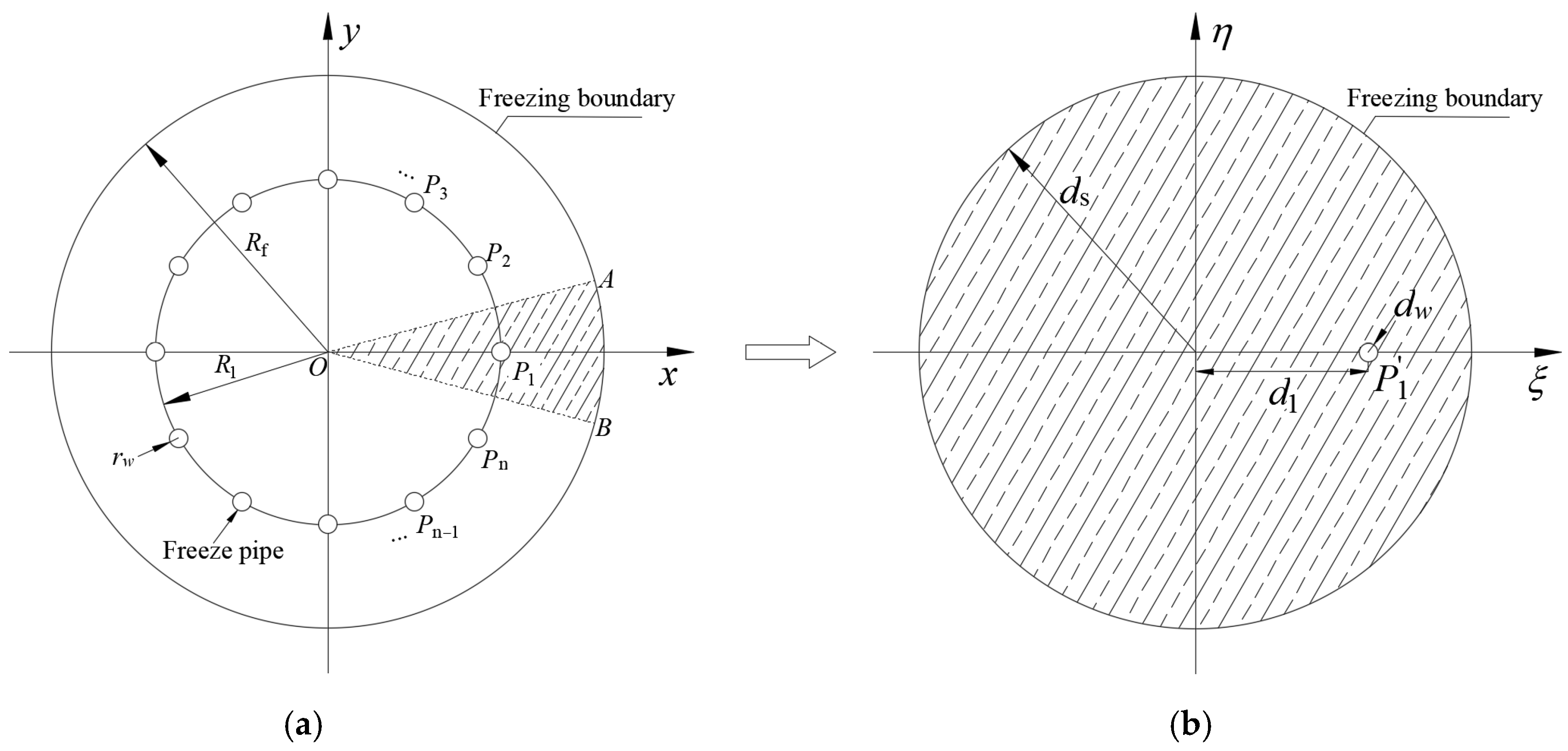
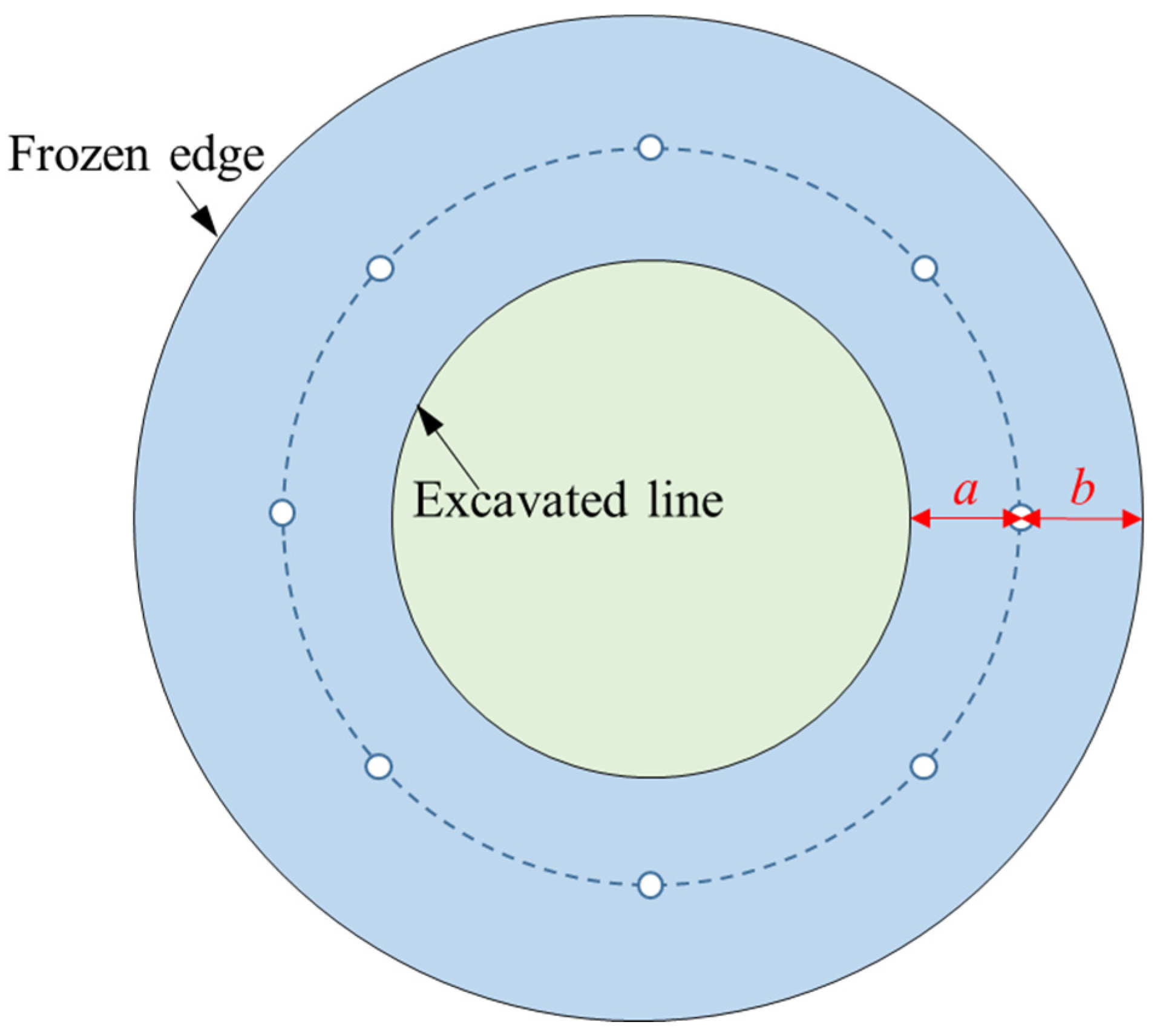
3.1. Description of Single-Circle Freezing Model

The most common annular layout of freezing pipes is the single-circle freezing model. Based on engineering experience, when the excavation section is small or frozen for a long time, the soil on the inside of the single-circle freezing pipes often all drops below the freezing point, such as in metro cross-passage projects and shaft-sinking projects. Although most of the freezing projects are not designed to freeze solid completely, but in some cases with long freezing time or small shaft diameter, the situation of a shaft completely frozen is still often encountered. Therefore, there are scholars suggesting that the excavation should be carried out after the shaft is completely frozen solid [26].

Meanwhile, it has been widely proved that undulation at the boundary of the frozen soil disappears shortly after the frozen soil column around each freezing pipe contacts each other, which is also called the closure of frozen wall in practical engineering, forming a smooth circular freezing boundary, as the different freezing condition in the early and later period of freezing process shown in Figure 3. So, this paper will focus on the condition that soil inside the freezing pipe ring is frozen solid completely and deduce an analytical solution to the static temperature field of this condition.

According to the above freezing condition with single-circle freezing pipes, we can build the following two-dimensional geometry model, n freezing pipes with the same wall temperature (T_f) and the same radius (r_w) are set evenly on a circumference whose radius is R₁, and the freezing pipe P₁ located on the x-axis, schematically shown in Figure 4a. Here we can assume that a circular frozen soil boundary (with a radius of R_f) forms around the ring of freezing pipes. The temperature at the boundary is T₀, which is also called the freezing point of the ground soil.

3.2. Conformal Mapping Function and Mapping Model

Considering the model symmetry in Figure 4a, we just need to consider the temperature field of a single freezing pipe located in a fan-shaped region of a central angle of 2π/n (∠AOB in Figure 4a). Then by choosing the appropriate conformal mapping function to convert the problem into the already solved condition of a circular stratum with an eccentric freezing pipe, as shown in Figure 4b, the expression formula of the potential of the single-circle freezing model can be deduced.

Here, we introduce the following conformal mapping formula to transform the real plane z(xoy) to the virtual plane ζ (ξoη):

$$\zeta =z^n$$

(8)

Define z = Re^iα, ζ = ρe^iθ, then substitute them into Formula (8), we obtain the following:

ρ = Rⁿ and θ = nα

(9)

It can be seen that by Formula (8), the angular region of a central angle of 2π/n in the z-plane is transformed to the angular region of a central angle of θ = n·2π/n = 2π in the ζ-plane. Additionally, the freezing pipe P₁, whose coordinates are r = R₁, α = 0 in the z-plane, is transformed to point P₁′, whose coordinates are d₁ = R₁ⁿ, θ₁= n·0 = 0 in the ζ-plane.

In addition, points at the freezing boundary in Figure 4a, which is a circumference of a radius of R_f in the z-plane, are mapped to points at a circumference of a radius of d_s = R_fⁿ in the ζ-plane. Additionally, the equivalent radius of the mapped freezing pipe can be calculated as follows:

$$d_{\mathrm{w}}=r_{\mathrm{w}}\cdot {\left|\frac{\mathrm{d}\zeta }{\mathrm{d}z}\right|}_{x=R_1}=n{R}_1{}^{n-1}{r}_{\mathrm{w}}$$

(10)

According to the principles of conformal mapping, by substituting d = Rⁿ (R is the polar radius of any point M in z-plane), d₁ = R₁ⁿ, θ = nα, d_w= nR₁ⁿ⁻¹r_w, d_s = R_fⁿ into Formulas (5) and (7), we can obtain the following expression formulas of Φ_M and q, which represent the potential of any point within the circular stratum concentric with a single-circle freezing pipes, and the heat flow volume of a single freezing pipe, respectively:

$${\Phi }_{\mathrm{M}}=\frac{q}{4\mathsf{\pi }}\ln \frac{{\left(\frac{R}{R_1}\right)}^n+{\left(\frac{R_1}{R}\right)}^n-2\cos n\alpha }{{\left(\frac{R{R}_1}{R_{\mathrm{f}}{}^2}\right)}^n+{\left(\frac{R_{\mathrm{f}}{}^2}{R{R}_1}\right)}^n-2\cos n\alpha }+{\Phi }_{\mathrm{s}}$$

(11)

$$q=\frac{2\mathsf{\pi }\left({\Phi }_{\mathrm{s}}-{\Phi }_W\right)}{\ln \left[-{\left(\frac{R_1}{R_{\mathrm{f}}}\right)}^n+\frac{R_s{}^n}{n{R}_1{}^{n-1}{r}_{\mathrm{w}}}-\frac{R_1{}^{2n}}{n{R}_1{}^{n-1}{R}_{\mathrm{f}}{}^n{r}_{\mathrm{w}}}\right]}$$

(12)

where α is the polar angle of a certain point M in the z-plane.

Substituting Formula (12) into Formula (11), we can obtain the expression of heat potential at any point in Figure 4a as follows:

$${\Phi }_{\mathrm{M}}=\left({\Phi }_{\mathrm{s}}-{\Phi }_W\right)\frac{\ln \frac{{\left(\frac{R}{R_1}\right)}^n+{\left(\frac{R_1}{R}\right)}^n-2\cos n\alpha }{{\left(\frac{R{R}_1}{R_{\mathrm{f}}{}^2}\right)}^n+{\left(\frac{R_{\mathrm{f}}{}^2}{R{R}_1}\right)}^n-2\cos n\alpha }}{2\ln \left[-{\left(\frac{R_1}{R_{\mathrm{f}}}\right)}^n+\frac{R_s{}^n}{n{R}_1{}^{n-1}{r}_{\mathrm{w}}}-\frac{R_1{}^{2n}}{n{R}_1{}^{n-1}{R}_{\mathrm{f}}{}^n{r}_{\mathrm{w}}}\right]}+{\Phi }_{\mathrm{s}}$$

(13)

3.3. Temperature Field with a Single-Circle Freezing Pipes

Based on the principle of similarity between thermodynamics and hydraulics, the flow volume of a well (q) is analogous to the heat flow volume of a freezing pipe, while the potential Φ_M is analogous to the product of temperature and thermal conductivity of the soil, i.e., Φ_M= KT. Assuming the temperature at the boundary of the frozen soil wall is T₀ = 0 °C, then the analytical formula of the static temperature field of ground with a single-circle freezing pipe can be figured out as the following Formula (14):

$$T\left(R,\alpha \right)=T_{\mathrm{f}}\cdot \frac{\ln \frac{{\left(\frac{R{R}_1}{R_{\mathrm{f}}{}^2}\right)}^n+{\left(\frac{R_{\mathrm{f}}{}^2}{R{R}_1}\right)}^n-2\cos n\alpha }{{\left(\frac{R}{R_1}\right)}^n+{\left(\frac{R_1}{R}\right)}^n-2\cos n\alpha }}{2\ln \left[-{\left(\frac{R_1}{R_{\mathrm{f}}}\right)}^n+\frac{R_{\mathrm{f}}{}^n}{n{R}_1{}^{n-1}{r}_{\mathrm{w}}}-\frac{R_1{}^{2n}}{n{R}_1{}^{n-1}{R}_{\mathrm{f}}{}^n{r}_{\mathrm{w}}}\right]}$$

(14)

where T(R, α) is the temperature of any points M(R, α) in the frozen soil wall, °C; T_f is the wall temperature freezing pipe, °C; R_f is the radius of the freezing boundary; R₁ is the radius of the freezing pipe circle; r_w is the radius of freezing pipes; n is the number of freezing pipes.

4. Accuracy Verification of Analytical Expression

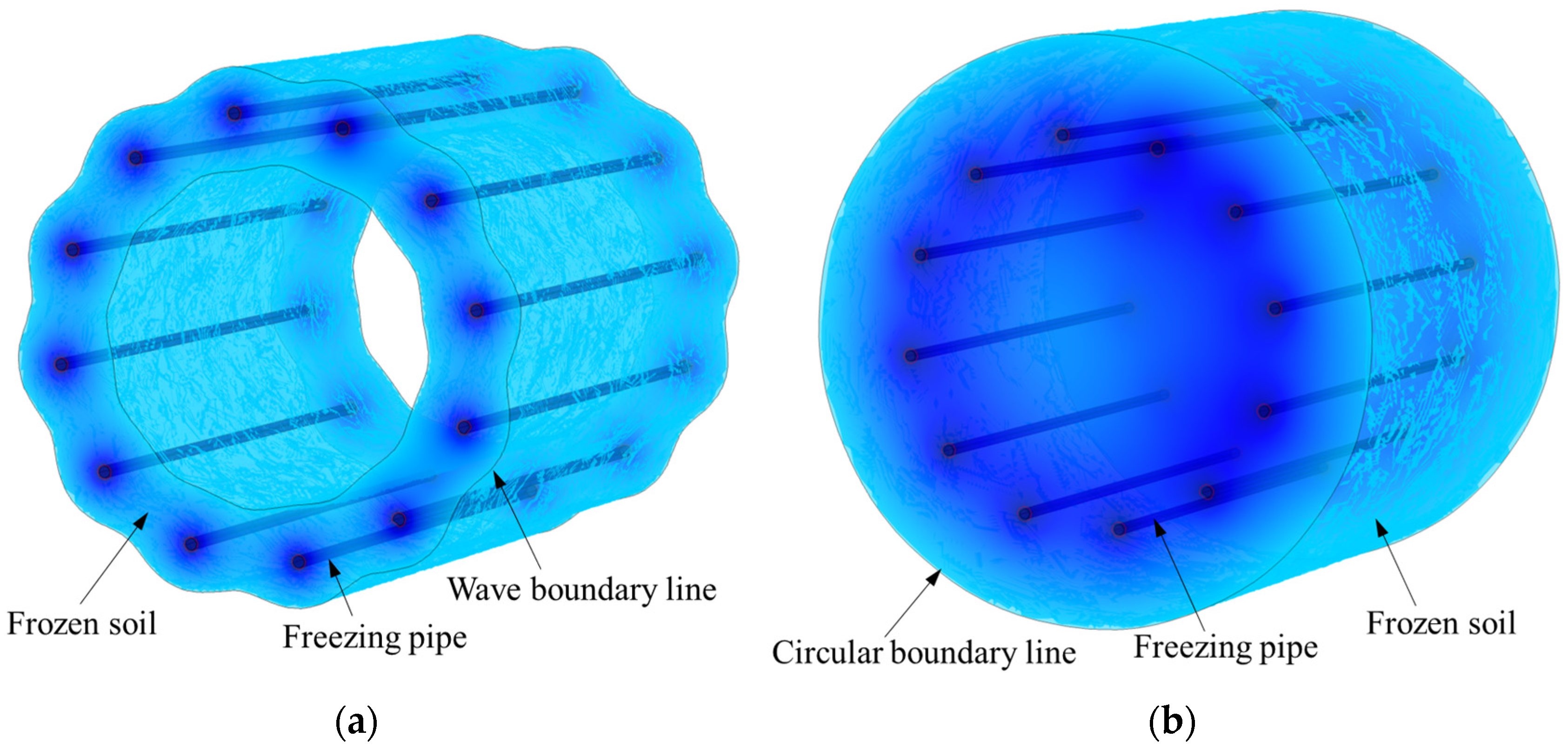
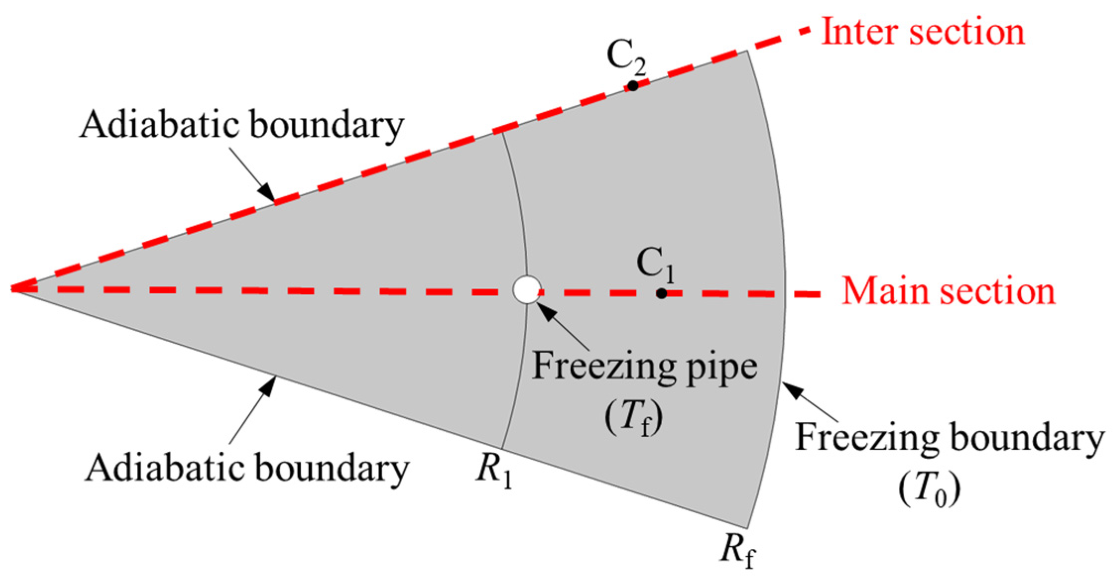
4.1. Numerical Model and Characteristic Sections

In order to verify the accuracy of the analytical expression (14) for the temperature field, this subsection employs steady-state numerical simulations for comparison. The heat transfer model is constructed using Comsol Multiphysics finite element software, and the boundary conditions, such as the freezing pipe wall temperature and soil freezing temperature, are in full agreement with the analytical derivation process. According to the geometric characteristics of the single-circle pipe freezing model, the periodic cell containing one freezing pipe is still selected here for calculation, and the numerical model is shown in Figure 5. Two characteristic cross-sections are also marked in this figure, one is referred to as the main section, which passes through the freezing pipe center, and the other is referred to as the inter section, which passes through the midpoint of the line connecting the adjacent freezing pipes.

4.2. Freezing Parameters

Given the same thermodynamic model and boundary conditions as the analytical method, numerical calculation of the temperature field is carried out, and the outcomes are compared with the results of the analytical calculation formula. Thus, it can be decided that, whether the application of the principle of similarity between thermodynamics and hydraulics here is reasonable, and whether the analytical formula can reflect the condition of the static temperature field accurately. According to the common freezing schemes in municipal engineering and mine engineering, the radius range of the frozen cross-section is generally in the range of 2 m ~ 6 m, and the spacing between adjacent freezing pipes is generally in the range of 0.6 m ~ 1.5 m, and the design frozen soil thickness is often within 2 m. In this work, multiple groups of parameters are adopted in numerical simulation; among them, four groups and their calculating results are chosen here to describe the outcome. These four groups of parameters are listed in

Table 1. Freezing parameters for comparative calculation.

Group	Number of Freezing Pipes n	Radius of Freezing Ring R1 (m)	Radius of Freezing Boundary Rf (m)	Freezing Pipes Spacing l (m)
1	10	2	3	1.26
2	20	2	3	0.63
3	25	6	7.5	1.51
4	50	6	7.5	0.75

. In Group 1 and Group 2, the thickness of the frozen soil outside the ring is 1 m, while in Group 3 and Group 4, the thickness is 1.5 m.

Appropriate simplification of the actual project is necessary before performing numerical calculations. In the numerical model of this paper, the important assumptions include three parts. First, the three-dimensional heat transfer process can be simplified to a two-dimensional planar problem because the axial temperature difference of the frozen tube is small. Secondly, it is assumed that the soil is isotropic material, and the difference in the distribution of material properties is not considered. Finally, the freezing tube wall temperature is assumed to be equal to the brine temperature, which has a small error for the freezing steady-state phase. Based on these assumptions, the static thermal conduction model is adopted for numerical calculation. According to practical conditions in engineering, the radius of all freezing pipes (r_w) was taken as 0.054 m. The wall temperature of the freezing pipes (T_f) is set to be −30 °C, and the temperature at the outer boundary of the frozen soil wall (T₀) is set to be 0 °C. The calculating region for numerical simulation is chosen to be a sector of a central angle of 360°/n, according to Figure 5. A free triangular mesh is adopted for the division of the computational area, the mesh grid is shown in Figure 6a, and the cloud map of temperature distribution is shown in Figure 6b.

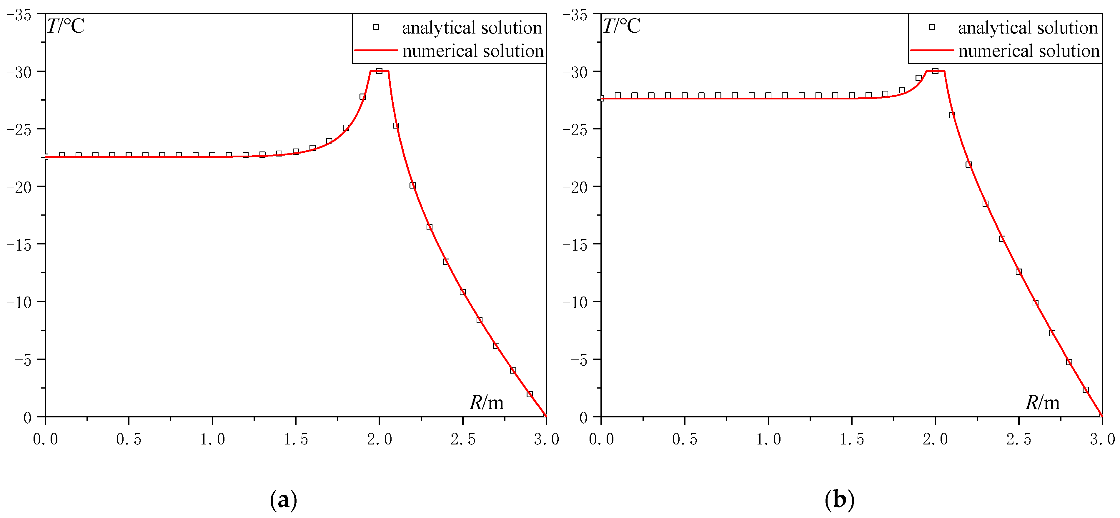
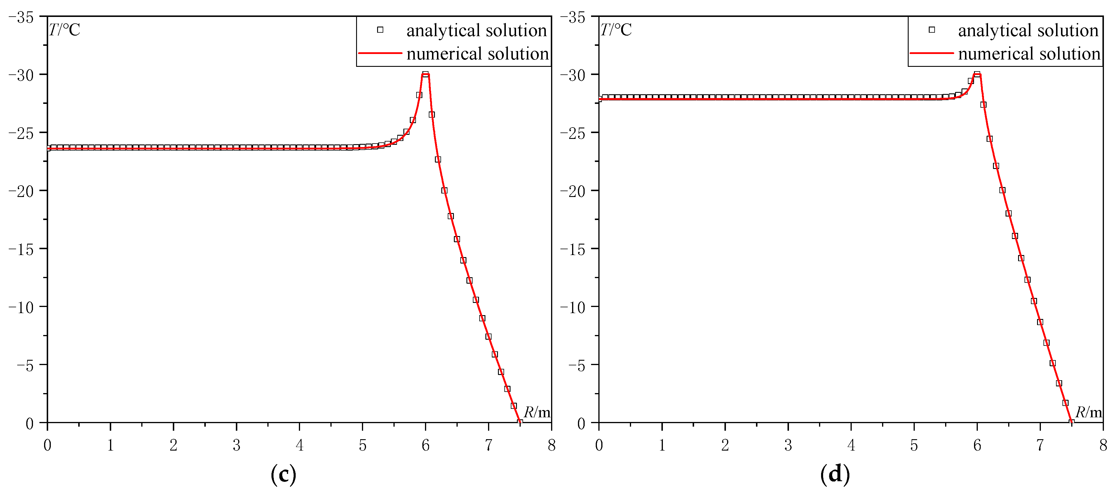
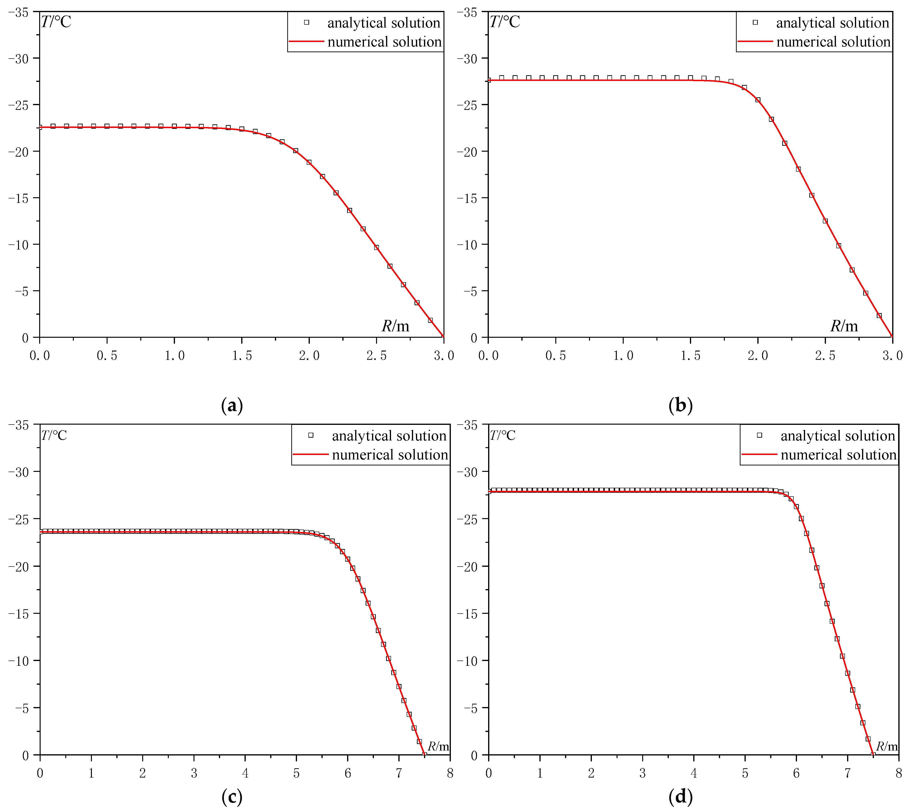
4.3. Temperature Distribution Curves

Substituting the freezing parameters in Table 1 into the analytical solution of the temperature field (14), the results of temperature distribution on the characteristic cross-section are obtained and then compared them with the numerical calculation results. The comparison curves of the characteristic section of numerical simulation with those of the analytical formula are shown in Figure 7 and Figure 8.

It can be concluded from Figure 7 and Figure 8 that the analytical calculation results of the temperature field are highly consistent with the numerical calculation results, and the temperature distribution curves are almost completely coincident, which shows that it is feasible to adopt a conformal transformation method to calculate the steady-state temperature field. The analytical solution (14) can well reflect the temperature distribution in the frozen soil cylinder formed by the annular layout of freezing pipes. In addition, it can also be found that the frozen soil temperature curve within R₁ is almost horizontal when the steady-state heat transfer state is reached, regardless of the size of the freezing pipe layout circle.

Considering the influence of different freezing parameters on temperature distribution in Table 1, it can be found from the comparison between Figure 7a,b that when the location of the freezing pipe is the same as the radius of the frozen soil column, the number of freezing pipes is doubled, and the temperature in the core area of the frozen soil column can be reduced by about 5 °C. When the frozen cross-section is enlarged, the temperature distribution of Group 3 and Group 4 also has this feature.

For the temperature comparison between two different characteristic sections, there is little difference in the temperature distribution between the main section and the inter section at the inner region of the circle ring of the freezing pipes. In the frozen soil area near the freezing pipe and R > R₁, the temperature gradient on these two characteristic sections is quite different. As the only cold source, the freezing pipe has an obvious effect on the temperature reduction near the pipe wall on the main section, and the minimum temperature can reach −30 °C, while the minimum temperature on the interface is generally between −25 °C and −25 °C according to the difference in the number of freezing pipes. The overall trend is that the temperature distributed in the main surface is lower than that in the inter section.

5. Simplification of Analytical Solution and Its Application

The temperature distribution within the frozen wall is the most concerning issue in engineering practice because it is closely related to the bearing strength and water-sealing performance of the frozen soil. The analytical solution of the temperature field is of great significance for freezing design and construction. Before introducing the application of the analytical solution, the analytical results will be suitably simplified based on the practical freezing project parameters in this chapter.

5.1. Simplified Analytical Expression

In the previous chapter, the temperature field distribution function of the annular arrangement of the freezing pipe is obtained, i.e., Equation (14). However, due to its complex expression, it may not be convenient for practical engineering applications. In order to use the analytical theory of temperature field to evaluate the freezing effect, this section simplifies the function form based on the actual freezing engineering experience parameters.

Observing the analytical Formula (14) for the temperature field, the denominator part can again be expressed in the following form:

$$-{\left(\frac{R_1}{R_s}\right)}^n+\frac{R_s{}^n}{n{R}_1{}^{n-1}{r}_{\mathrm{w}}}-\frac{R_1{}^{2n}}{n{R}_1{}^{n-1}{R}_{\mathrm{f}}{}^n{r}_{\mathrm{w}}}=-{\left(\frac{R_1}{R_s}\right)}^n+\frac{R_s{}^n}{n{R}_1{}^{n-1}{r}_{\mathrm{w}}}\left[1-{\left(\frac{R_1}{R_{\mathrm{f}}}\right)}^n\right]$$

In practical freezing engineering, since there must be a conclusion that the radius of the freezing pipe layout circle is far less than the radius of the outer frozen soil curtain; that is, R₁ < R_f, the following conclusions always hold: R₁ⁿ/R_fⁿ < < 1, R₁²ⁿ/R_f²ⁿ < < 1, (RR₁)ⁿ/R_f²ⁿ < < 1. Then, for the convenience of calculation in the specific project, the temperature field expression Formula (14) can also be simplified as follows:

$$T\left(R,\alpha \right)=\frac{T_{\mathrm{f}}}{2\ln \left(\frac{R_{\mathrm{f}}{}^n}{n{R}_1{}^{n-1}{r}_{\mathrm{w}}}\right)}\cdot \ln \frac{{\left(\frac{R_{\mathrm{f}}{}^2}{R{R}_1}\right)}^n-2\cos n\alpha }{{\left(\frac{R}{R_1}\right)}^n+{\left(\frac{R_1}{R}\right)}^n-2\cos n\alpha }$$

(15)

In order to verify the accuracy of the simplified analytical solution under different freezing conditions, the simplified solution (15) is compared with the non-simplified solution (14) based on the four groups of parameters in Table 1. Select the C₁ point on the main section and the C₂ point on the inter section for comparison. These two points are located in the middle of the freezing pipe layout circle and the outer boundary of frozen soil; that is, polar diameter R = (R₁ + R_f)/2. The schematic diagram of the two points’ positions is shown in Figure 5, and the error calculation results are shown in

Table 2. Calculation errors of simplified and non-simplified analytical solution (/℃).

Group	C1			C2
	Equation (14)	Equation (15)	Error 1	Equation (14)	Equation (15)	Error 2
1	−23.0021	−23.0012	0.0009	−22.3717	−22.3708	0.0009
2	−27.8923	−27.8923	0	−27.8705	−27.8705	0
3	−11.4047	−11.4047	0	−10.96	−10.96	0
4	−13.2258	−13.2258	0	−13.2119	−13.2119	0

.

According to Table 2, it can be found that the simplified solution of the temperature field obtained based on the practical engineering freezing parameters is very accurate, and the error between the simplified solution and the non-simplified solution is very small, less than 1/‰. Formula (15) can fully meet the use requirements of the field of engineering. Therefore, in the application of the analytical solution of the temperature field in the following paper, all the calculations in this paper are based on the simplified analytical expression (15).

5.2. Frozen Soil Thickness Based on Measured Temperature

The thickness index of the frozen wall is closely related to its load-bearing strength, after obtaining the analytical expression of temperature field distribution, it is very convenient in practical engineering to calculate the thickness of frozen soil wall based on temperature data of measuring points.

Suppose there is a point M in the calculation range of the freezing model in Figure 4a, and its position information is expressed as (R_M, α_M) using polar coordinates. In practical engineering, the temperature sensor is used to obtain its temperature as T_M, then it must meet the analytical expression of temperature field distribution; that is, T_M = T (R_M, α_M). Substituting it into the simplified solution of temperature field (15), we can obtain the following:

$$T_M=\frac{T_{\mathrm{f}}}{2\ln \left(\frac{R_{\mathrm{f}}{}^n}{n{R}_1{}^{n-1}{r}_{\mathrm{w}}}\right)}\cdot \ln \frac{{\left(\frac{R_{\mathrm{f}}{}^2}{R_M{R}_1}\right)}^n-2\cos \left(n{\alpha }_M\right)}{{\left(\frac{R_M}{R_1}\right)}^n+{\left(\frac{R_1}{R_M}\right)}^n-2\cos \left(n{\alpha }_M\right)}$$

(16)

In fact, there is only one unknown parameter in Equation (16), i.e., R_f. The value of the frozen curtain thickness can be calculated by solving the following Equation (16):

R_f = f (R₁, R_M, r_w, α_M, T_f, T_M, n)

Furthermore, if the measurement point M is arranged near the outer edge of the frozen curtain, then there must be (R_M /R₁) ⁿ > 2 under the condition of multi-pipe freezing. Considering that (R_f ² /R_M R₁) ⁿ > 2 always holds, the effect of the pole angle α can be neglected in Equation (16), and the temperature of the point M can again be expressed in relation to the coordinates as follows:

$$T_M=\frac{T_{\mathrm{f}}}{2\ln \left(\frac{R_{\mathrm{f}}{}^n}{n{R}_1{}^{n-1}{r}_{\mathrm{w}}}\right)}\cdot \ln \frac{R_{\mathrm{f}}{{}^2}^n}{R_M{{}^2}^n+R_1{{}^2}^n}$$

(17)

According to Equation (17), the frozen soil thickness can be explicitly expressed as follows:

$$R_{\mathrm{f}}=\exp \left[\frac{2T_M\ln \left(n{R}_1{}^{n-1}{r}_{\mathrm{w}}\right)-T_{\mathrm{f}}\ln \left(R_M{{}^2}^n+R_1{{}^2}^n\right)}{2n\left(T_M-T_{\mathrm{f}}\right)}\right]$$

(18)

5.3. Average Temperature of Frozen Wall

In engineering practice, we also need to calculate the average temperature of the unexcavated frozen soil, so it is necessary to derive a formula to obtain the average temperature with the previous analytical results. We named the distance between the freezing pipe circle and excavated face as a and the thickness of the frozen wall on the outside of the freezing pipe circle as b; thus, the thickness of the unexcavated frozen wall is (a + b). The distribution of frozen soil thickness inside and outside the frozen circle is shown in Figure 9.

According to Figure 7 and Figure 8, the temperature field is different between the main section and inter section. Combined with the analytical solution (see Formula (14)), it is not difficult to know that the temperature field in the other radial section is between the condition in the main section and inter section. So, the average temperature of the frozen wall cannot be represented by the value of the main section or the inter section. Instead, it should be the same with the average temperature of one radial section between the main section and the inter section.

As shown in Figure 7 and Figure 8, broken line BAD nearly divides the area equally between the temperature curve of the main section and the inter section. So, from the geometric schematic of the frozen soil distribution after excavation, it is a feasible method that divides the area of the right trapezoid ABCD by the thickness of the frozen wall to calculate the average temperature.

In Figure 10, the temperature of point A is equal to the temperature in the center of pipe circle, and it can be expressed as follows:

$$T_A=\frac{T_{\mathrm{f}}}{2\ln \left(\frac{R_{\mathrm{f}}{}^n}{n{R}_1{}^{n-1}{r}_{\mathrm{w}}}\right)}\cdot \ln \frac{R_{\mathrm{f}}{}^{2n}}{R_1{}^{2n}}$$

(19)

Then, dividing the area of right trapezoid ABCD by the thickness of frozen wall (a + b), we can obtain the following formula of average temperature in frozen wall:

$$T_{\mathrm{average}}=\frac{1}{2}\cdot \frac{a+\left(a+b\right)}{a+b}\cdot \frac{T_{\mathrm{f}}}{2\ln \left(\frac{R_{\mathrm{f}}{}^n}{n{R}_1{}^{n-1}{r}_{\mathrm{w}}}\right)}\cdot \ln \frac{R_{\mathrm{f}}{}^{2n}}{R_1{}^{2n}}$$

(20)

6. Conclusions

Based on the common annular freezing scheme in the artificial ground freezing method, considering the complete frozen state inside the freezing circle, the analytical expression of the steady-state temperature field is solved by the hydraulic potential and complex function method. The main conclusions are as follows:

(1)

The potential function in hydraulics and the temperature potential function in thermodynamics are essentially the same, and the method of solving concentric wells using eccentric wells combined with the conformal transformation method can also be adopted to derive for the temperature field distribution with an annular layout of freezing pipes;

(2)

Through numerical simulation of the static temperature field of ground with single-circle freezing pipes, the analytical formula is verified to be accurate enough. The results show the analytical formula can reflect the condition of the temperature field very well;

(3)

After simplifying the analytical expression based on the dimensional parameters of the actual freezing project, the calculating results by the simplified formula are very close to that by non-simplified analytical formula with negligible errors;

(4)

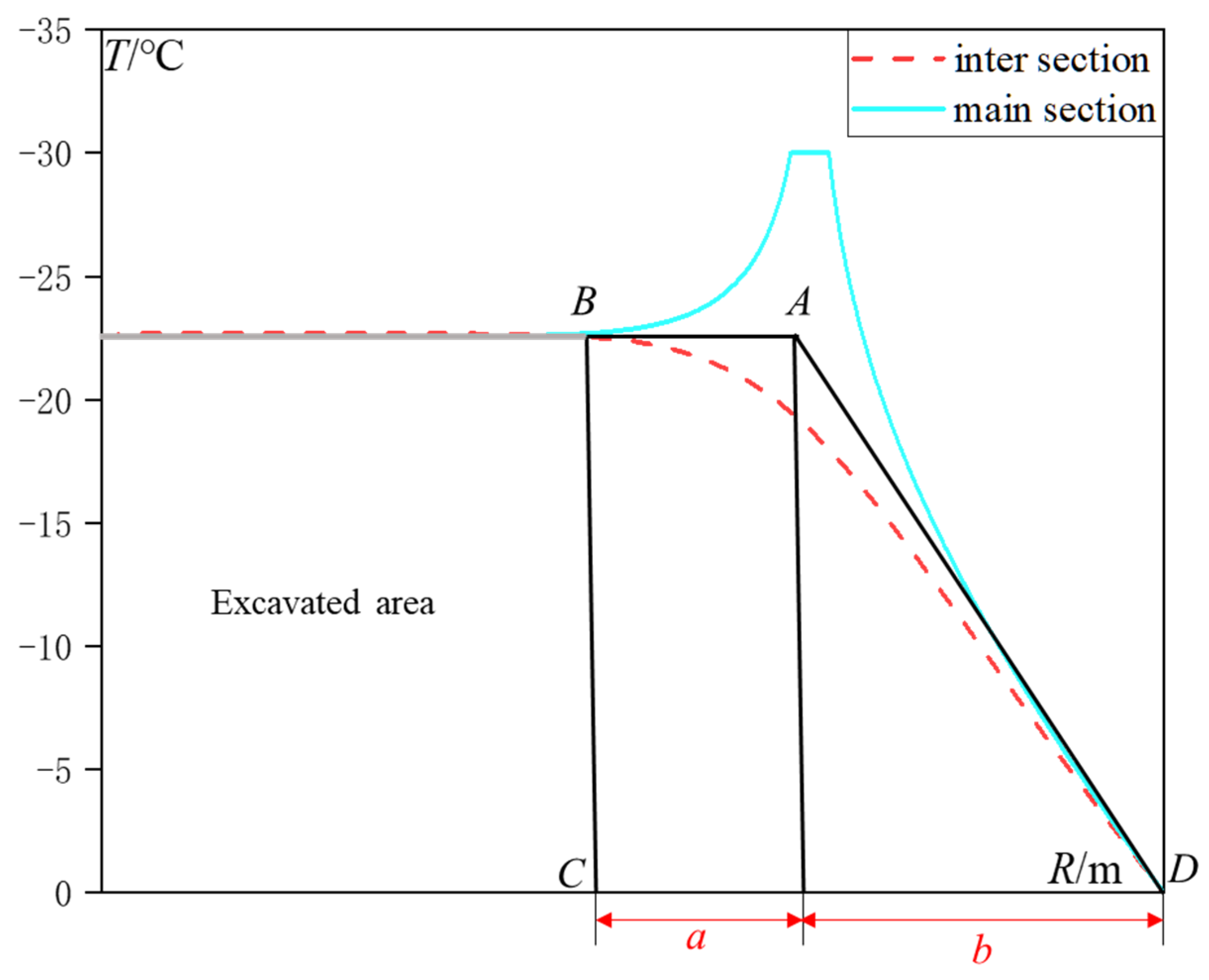
In the region close to the freezing pipe circle, the main section temperature is much lower than the inter section temperature, but they are nearly the same near the cross-section center. It is convenient to calculate the thickness and average temperature of the frozen column using the formula expression of the temperature field.

It is worth mentioning that since the periodicity of the annular arrangement of freezing pipes is used in the derivation of the analytical solution in this paper, the deflection of freeze holes in actual projects cannot be considered yet, and further research in this aspect is needed in the future.

References

1. Chen, R.J.; Cheng, G.D.; Li, S.X.; Guo, X.M.; Zhu, L.N. Development and prospect of research on application of artificial ground freezing. Chin. J. Geotech. Eng. 2000, 1, 43–47. [Google Scholar]
2. Chen, X.S. Several key points of artificial ground freezing method and its latest application in China. Tunn. Constr. 2015, 35, 1243–1251. [Google Scholar]
3. Casini, F.; Gens, A.; Olivella, S. Artificial ground freezing of a volcanic ash: Laboratory tests and modelling. Environ. Geotech. 2014, 3, 141–154. [Google Scholar] [CrossRef]
4. Wang, R.H.; Wang, W. Analysis for features of the freezing temperature field under deflective pipes. Chin. J. Geotech. Eng. 2003, 25, 658–661. [Google Scholar]
5. Sanger, F.C.; Sayles, F.H. Thermal and rheological computations for artificially frozen ground construction. Eng. Geol. 1979, 13, 311–337. [Google Scholar] [CrossRef]
6. Trupak, N.G. Ground Freezing in Shaft Sinking; Coal Technology Press: Moscow, Russia, 1954. (In Russian) [Google Scholar]
7. BaKholdin, B.V. Selection of Optimized Mode of Ground Freezing for Construction Purpose; State Construction Press: Moscow, Russia, 1963. (In Russian) [Google Scholar]
8. Hu, X.D.; Huang, F.; Bai, N. Models of artificial frozen temperature field considering soil freezing point. J. China Univ. Min. Technol. (Nat. Sci.) 2008, 37, 550–555. (In Chinese) [Google Scholar]
9. Hu, X.D.; Guo, W.; Zhang, L.Y. Analytical solution of steady state temperature field of a few freezing pipes in infinite region. J. China Coal Soc. 2013, 38, 1953–1960. [Google Scholar]
10. Hu, X.D.; Zhao, J.J. Research on Precision of Bakholdin model for Temperature Field of Artificial Ground Freezing. Chin. J. Undergr. Space Eng. 2010, 6, 96–101. (In Chinese) [Google Scholar]
11. Hu, X.D.; Zhang, L.Y. Analytical solution to steady-state temperature field of two freezing pipes with different temperatures. J. Shanghai Jiaotong Univ. (Sci.) 2013, 18, 706–711. [Google Scholar] [CrossRef]
12. Hu, C.P.; Hu, X.D.; Zhu, H.H. Sensitivity analysis of control parameters of Bakholdin solution in single-row-pipe freezing. J. China Coal Soc. 2011, 36, 938–944. (In Chinese) [Google Scholar]
13. Huang, Z.K.; Zhang, D.M.; Pitilakis, K.; Tsinidis, G.; Argyroudis, S. Resilience assessment of tunnels: Framework and application for tunnels in alluvial deposits exposed to seismic hazard. Soil Dyn. Earthq. Eng. 2022, 162, 107456. [Google Scholar] [CrossRef]
14. Zhang, J.Z.; Phoon, K.K.; Zhang, D.M.; Huang, H.W.; Tang, C. Novel approach to estimate vertical scale of fluctuation based on CPT data using convolutional neural networks. Eng. Geol. 2021, 294, 106342. [Google Scholar] [CrossRef]
15. Zhang, J.Z.; Huang, H.W.; Zhang, D.M.; Phoon, K.K.; Liu, Z.Q.; Tang, C. Quantitative evaluation of geological uncertainty and its influence on tunnel structural performance using improved coupled Markov chain. Acta Geotech. 2021, 16, 3709–3724. [Google Scholar] [CrossRef]
16. Hu, X.D.; Fang, T.; Han, Y.G. Mathematical solution of steady-state temperature field of circular frozen wall by single-circle-piped freezing. Cold Reg. Sci. Technol. 2018, 148, 96–103. [Google Scholar] [CrossRef]
17. Hu, X.D.; Wang, Y. Analytical Solution of Three-row-piped Frozen Temperature Field by Means of Superposition of Potential Function. Chin. J. Rock Mech. Eng. 2012, 31, 1071–1080. [Google Scholar]
18. Wang, Y.; Tan, P.F.; Han, J.; Li, P. Energy-driven fracture and instability of deeply buried rock under triaxial alternative fatigue loads and multistage unloading conditions: Prior fatigue damage effect. Int. J. Fatigue 2023, 168, 107410. [Google Scholar] [CrossRef]
19. Wang, Y.; Yan, M.Q.; Song, W.B. The effect of cyclic stress amplitude on macro-meso failure of rock under triaxial confining pressure unloading. Fatigue Fract. Eng. Mater. Struct. 2023, 47, 3008–3025. [Google Scholar] [CrossRef]
20. Lukyanov, V.S. Study and calculations of the temperature regime of the ground and structures by the hydraulic analog method. In Proceedings of the Permafrost: Second International Conference, Yakutsk, Russia, 12–20 July 1973; pp. 807–908. [Google Scholar]
21. Huang, Z.K.; Argyroudis, S.; Zhang, D.M.; Pitilakis, K.; Huang, H.W.; Zhang, D.M. Time-dependent fragility functions for circular tunnels in soft soils. ASCE-ASME J. Risk Uncertainty Eng. Syst. Part A: Civ. Eng. 2022, 8, 04022030. [Google Scholar] [CrossRef]
22. Ge, J.L. Modern Reservoir Seepage Flow Mechanics Principle; Petroleum Industry Press: Beijing, China, 2001. (In Chinese) [Google Scholar]
23. Li, X.P. The Oil and Gas Flow through Porous Media; Petroleum Industry Press: Beijing, China, 2008. (In Chinese) [Google Scholar]
24. Charny, Y.A. Underground Hydro Gas Dynamics; Gostoptekhizdat: Moscow, Russia, 1982. (In Russian) [Google Scholar]
25. Li, X.; Chen, J.B. Oil and Gas Percolation Mechanics: English; Petroleum Industry Press: Beijing, China, 2012. [Google Scholar]
26. Cheng, H.; Cai, H.B. Safety situation and thinking about deep shaft construction with freezing method in China. J. Anhui Univ. Sci. Technol. (Nat. Sci.) 2013, 33, 1–6. [Google Scholar]
Figure 1. Potential function model of the well at the origin.
Mathematics 11 01962 g001
Figure 2. Potential function model with an eccentric well.
Mathematics 11 01962 g002
Figure 3. Two frozen conditions in the early and later period of freezing process: (a) early period; (b) later period.
Mathematics 11 01962 g003
Figure 4. Single-circle freezing model and its mapping model: (a) single-circle freezing model (b) mapping model with an eccentric freezing pipe P1.
Mathematics 11 01962 g004
Figure 5. Numerical model and characteristic sections.
Mathematics 11 01962 g005
Figure 6. Mesh division and temperature cloud map by numerical calculation: (a) mesh grid; (b) temperature cloud.
Mathematics 11 01962 g006
Figure 7. Comparison curves of analytical and numerical solutions in main section: (a) group 1; (b) group 2; (c) group 3; (d) group 4.
Mathematics 11 01962 g007aMathematics 11 01962 g007b
Figure 8. Comparison curves of analytical and numerical solutions in inter section: (a) group 1; (b) group 2; (c) group 3; (d) group 4.
Mathematics 11 01962 g008
Figure 9. Distribution diagram of frozen soil thickness after excavation.
Mathematics 11 01962 g009
Figure 10. Schematic diagram of average temperature calculation method.
Mathematics 11 01962 g010