Unconditional Superconvergence Error Estimates of Semi-Implicit Low-Order Conforming Mixed Finite Element Method for Time-Dependent Navier–Stokes Equations

Abstract

In this paper, the unconditional superconvergence error analysis of the semi-implicit Euler scheme with low-order conforming mixed finite element discretization is investigated for time-dependent Navier–Stokes equations. In terms of the high-accuracy error estimates of the low-order finite element pair on the rectangular mesh and the unconditional boundedness of the numerical solution in $L^{\infty }$-norm, the superclose error estimates for velocity in $H^1$-norm and pressure in $L^2$-norm are derived firstly by dealing with the trilinear term carefully and skillfully. Then, the global superconvergence results are obtained with the aid of the interpolation post-processing technique. Finally, some numerical experiments are carried out to support the theoretical findings.

1. Introduction

In this paper, we consider the following two-dimensional time-dependent incompressible Navier–Stokes equations:

$$\begin{array}{cc}\hfill & {\mathit{u}}_t-\Delta \mathit{u}+(\mathit{u}·\nabla )\mathit{u}+\nabla p=\mathit{f},(\mathit{x},t)\in \mathsf{\Omega }\times (0,T],\hfill \end{array}$$

(1)

$$\begin{array}{cc}\hfill & \nabla ·\mathit{u}=0,(\mathit{x},t)\in \mathsf{\Omega }\times (0,T],\hfill \end{array}$$

(2)

$$\begin{array}{cc}\hfill & \mathit{u}(\mathit{x},t)=0,(\mathit{x},t)\in \partial \mathsf{\Omega }\times (0,T],\hfill \end{array}$$

(3)

$$\begin{array}{cc}\hfill & \mathit{u}(\mathit{x},0)={\mathit{u}}_0\left(\mathit{x}\right),\mathit{x}\in \mathsf{\Omega },t=0,\hfill \end{array}$$

(4)

where $\mathsf{\Omega }\subset {\mathbb{R}}^2$ is a rectangular domain with boundary $\partial \mathsf{\Omega }$, $\mathit{u}=(u_1,u_2)=(u_1\left(\mathit{x}\right),u_2\left(\mathit{x}\right))$ represents the velocity vector, $p=p\left(\mathit{x}\right)$ denotes the pressure, and $\mathit{f}=(f_1\left(\mathit{x}\right),f_2\left(\mathit{x}\right))$ is the prescribed body force, $\mathit{x}=(x,y)$. Moreover, ${\mathit{u}}_0$ is the initial velocity and $T>0$ is the final time.

Navier–Stokes equations are a classical incompressible fluid model and have been widely applied in the mathematical physics and the computational fluid dynamics fields [1,2,3]. It is an unrealistic thing to find the the exact solutions of the Navier–Stokes equations due to their nonlinear and incompressible properties. Therefore, numerous works have been devoted to the development of efficient numerical approximations for Navier–Stokes Equations (1)–(4), including finite difference methods [4,5,6,7], Galerkin finite element methods [8,9,10,11,12,13,14,15,16,17,18,19,20,21] and other methods [22,23,24,25,26]. In particular, a new second-order accurate finite difference scheme for the incompressible Navier–Stokes equations was discussed in [4] by the primitive variable formulation. Based on the vorticity stream-function formulation and a fast Poisson solver defined on a general domain using the immersed interface method, a fast finite difference method was proposed and studied in [5] for the incompressible Navier–Stokes equations. A new fully discrete finite element nonlinear Galerkin method was established in [8] for the Navier–Stokes equations with two-grid finite element discretization in the spatial direction and Euler explicit scheme with variable time step size in the temporal direction. The boundedness, convergence and stability condition of the presented method were discussed under certain time-step constraints dependent on the coarse grid parameter. A Lagrange–Galerkin mixed finite element approximation was presented for the Navier–Stokes equations in [13], and optimal error estimates were obtained with the mesh restriction $\tau =O\left(h^{\sigma }\right)$, where $\sigma >(d-1)/2$, and $\tau$, h and d denote the time step size, the mesh size and the dimension of the domain, respectively. In [14], in terms of the special properties of a low-order nonconforming mixed finite element pair on the rectangular mesh, the superconvergence error estimates were derived for Navier–Stokes equations with the time-step constraints $\tau =O\left(h^{1+\alpha }\right)$, $\alpha >0$ due to the inverse inequality used in the error analysis. In [18], in terms of the error splitting technique developed in [27,28], the unconditional stability and convergence of a typical modified characteristics finite element method were studied for the time-dependent Navier–Stokes equations by introducing an iterated characteristic time-discrete system. Optimal error estimates were obtained under the boundedness of the numerical solution in $W^{1,\infty }$-norm. Subsequently, the unconditionally optimal error estimates were derived in [20] under the boundedness of the numerical solution in $L^{\infty }$-norm, which is weaker than that in [18].

It should be pointed out that optimal error estimates were obtained in [20] due to roughly handling trilinear terms. Moreover, the superconvergence error estimates were derived in [14] with a certain time-step restriction. To the best of our knowledge, there are few contributions on the unconditionally superclose and superconvergence error estimates for problems (1)–(4). The purpose of this paper is to consider the unconditionally superclose and superconvergence error estimates for incompressible time-dependent Navier–Stokes Equations (1)–(4). It should be pointed out that the difficulties come from the trilinear term (i.e., the convection term) $(\mathit{u}·\nabla )\mathit{u}$ in the superclose and superconvergence error analysis. Therefore, we should deal with them carefully and skillfully.

In the present work, we focus on a low-order conforming finite element approximation, which is called the bilinear-constant scheme [4,29,30], for problems (1)–(4). The key to our analysis is to employ the special properties (high-accuracy error estimation; see Lemmas 1–2 below) on the rectangular mesh and to treat the convection term $(\mathit{u}·\nabla )\mathit{u}$ rigorously and skillfully. The superclose error estimates are obtained firstly for the velocity in $H^1$-norm and for the pressure in $L^2$-norm. Then, in terms of an efficient interpolation post-processing approach, the global superconvergence results are derived for the velocity in the $H^1$-norm and for the pressure in the $L^2$-norm. In addition, some numerical experiments are presented and tested.

The remainder of this paper is organized as follows. In Section 2, some preliminaries and lemmas are introduced, and the semi-implicit Euler fully discrete finite element approximation of the problem (1)–(4) is presented. In Section 3, the detailed superclose error estimates are studied with the help of the special properties of the bilinear-constant finite element pair combined with skillfully dealing with the trilinear term. Then, the global superconvergence error estimates are established by the interpolation post-processing technique. In Section 4, some numerical results are provided to verify the theoretical findings.

2. Preliminaries

We denote by $W^{m,p}\left(\mathsf{\Omega }\right)$ the Sobolev spaces with the norm ${\parallel ·\parallel }_{m,p}$ and semi-norm ${|·|}_{m,p}$ defined by

$${\parallel u\parallel }_{m,p}=\left\{\begin{array}{cc}{\left(\sum _{\left|\beta \right|\le k}{\int }_{\mathsf{\Omega }}{\left|D^{\beta }u\right|}^{p}dxdy\right)}^{\frac{1}{p}},\hfill & 1\le p<\infty ,\hfill \\ \\ \sum _{\left|\beta \right|\le k}{\mathrm{e}\mathrm{s}\mathrm{s}\mathrm{s}\mathrm{u}\mathrm{p}}_{\mathsf{\Omega }}\left|D^{\beta }u\right|,\hfill & p=\infty ,\hfill \end{array}\right.$$

where $D^{\beta }=\frac{{\partial }^{\left|\beta \right|}}{\partial x^{{\beta }_1}\partial y^{{\beta }_2}}$ for the multi-index $\beta =({\beta }_1,{\beta }_2)$, ${\beta }_1\ge 0$, ${\beta }_2\ge 0$ and $\left|\beta \right|={\beta }_1+{\beta }_2$. For $p=2$, we let $H^m\left(\mathsf{\Omega }\right)$ denote $W^{m,2}\left(\mathsf{\Omega }\right)$. We omit the subscript when $p=2$ and write ${\parallel ·\parallel }_{0,2}$ and ${|·|}_{0,2}$ as ${\parallel ·\parallel }_0$ and ${|·|}_0$ for simplicity. Moreover, we use $(·,·)$ to represent the $L^2$ inner product, i.e.,

$$\begin{array}{c}\hfill (u,v)={\int }_{\mathsf{\Omega }}uvdxdy.\end{array}$$

For the mathematical setting of the problem (1)–(4), we introduce the following Sobolev spaces $\mathit{V}$ and M [31], i.e.,

$$\begin{array}{c}\hfill \mathit{V}={\left(H_0^1\left(\mathsf{\Omega }\right)\right)}^2,P=L_0^2\left(\mathsf{\Omega }\right)=\{q\in L^2\left(\mathsf{\Omega }\right):{\int }_{\mathsf{\Omega }}qdxdy=0\}.\end{array}$$

Moreover, for any Banach space X and $I=[0,T]$, let $L^p(I;X)$ be the space of all measurable function $f:I\to X$ with the norm

$${\parallel f\parallel }_{L^p(I;X)}=\left\{\begin{array}{cc}({\int }_0^T{\parallel f\parallel }_X^p{dt)}^{\frac{1}{p}},\hfill & 1\le p\le \infty ,\hfill \\ \mathrm{ess}{\sup }_{t\in I}{\parallel f\parallel }_X,\hfill & p=\infty .\hfill \end{array}\right.$$

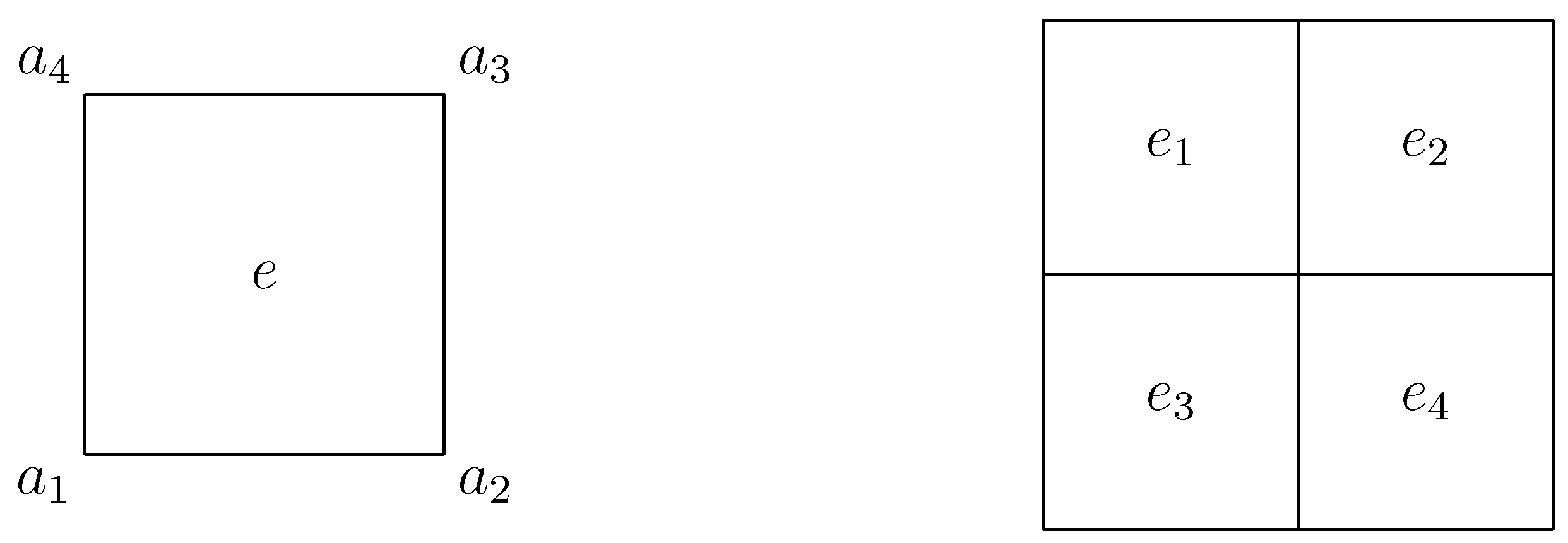
Let ${\mathcal{T}}_h=\left\{e\right\}$ be a uniform rectangular mesh over $\mathsf{\Omega }$ with mesh size h. For a given element $e\in {\mathcal{T}}_h$, its four vertices are denoted by $a_i(x_i,y_i),i=1,2,3,4$ in the counterclockwise order (see Figure 1 left). For the velocity, we choose ${\mathit{V}}_h$ as the general bilinear finite element space. For the pressure, we assume that the subdivision ${\mathcal{T}}_h$ is obtained from ${\mathcal{T}}_{2h}=\left\{\tau \right\}$ by dividing each element of ${\mathcal{T}}_{2h}$ into four small congruent rectangles. 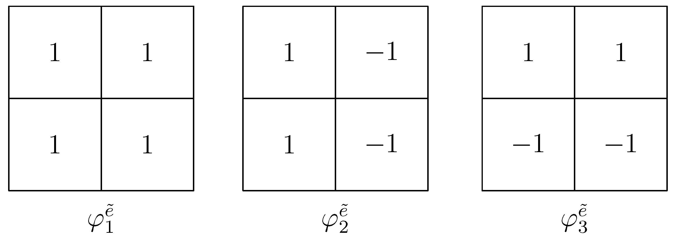Let $P_h^{{}^{\prime }}$ consist of piecewise constant functions with respect to ${\mathcal{T}}_h$ such that the local basis functions for $P_h^{{}^{\prime }}$ on a $2\times 2$-patch of $\tau$ (see Figure 1 right) are indicated in Figure 2. Then, the finite element space for pressure is defined by $P_h^{{}^{\prime }}\cap L_0^2\left(\mathsf{\Omega }\right)$. In the following discussion, we always assume that $\tau ={\cup }_{i=1}^4{e}_i\in {\mathcal{T}}_{2h}$ with $e_i\in {\mathcal{T}}_h(1\le i\le 4)$ (see Figure 1 right). Thus, the finite element approximation spaces ${\mathit{V}}_h$ and $M_h$ for the bilinear-constant scheme are described by ([1,29,30])

$$\begin{array}{cc}\hfill & {\mathit{V}}_h=\{\mathit{v}\in {\left(C\left(\overline{\mathsf{\Omega }}\right)\right)}^2{:\mathit{v}|}_e\in {\left(Q_{11}\left(e\right)\right)}^2,\mathit{v}{|}_{\partial \mathsf{\Omega }}=0,e\in {\mathcal{T}}_h\},\hfill \\ \hfill & M_h=\{p\in L_0^2\left(\mathsf{\Omega }\right):p{|}_{\tau }=\sum _{i=1}^3{\lambda }_i^{\tau }{\phi }_i^{\tau },\sum _{\tau \in {\mathcal{T}}_{2h}}{\lambda }_1^{\tau }=0,\tau \in {\mathcal{T}}_{2h}\},\hfill \end{array}$$

where $Q_{11}$ denotes the space of all polynomials of degree $\le 1$ with respect to each of the two variables, x and y. It is shown in [1,29,30] that the bilinear-constant scheme satisfies the Babuška–Brezzi condition, i.e.,

$$\begin{array}{c}\hfill \underset{0\ne {\mathit{v}}_h\in {\mathit{X}}_h}{sup}\frac{(q_h,\nabla ·{\mathit{v}}_h)}{\parallel {\mathit{v}}_h{\parallel }_1}\ge \beta {\parallel q_h\parallel }_0,\forall q_h\in M_h,\end{array}$$

(5)

where $\beta >0$ is a constant, independent of h.

Figure 1. The element $e$(left) and $\tilde{e}$(right).

Figure 2. Local basis functions of $P_h^{{}^{\prime }}$.

For the velocity, we use the Lagrange nodal interpolation operator $I_h:{\left(C\left(\overline{\mathsf{\Omega }}\right)\right)}^2\mapsto {\mathit{V}}_h$ as the corresponding interpolation operator. For the pressure, we first introduce the local $L^2$-projection $J_h^{{}^{\prime }}p$ of p by

$$\begin{array}{c}\hfill J_h^{{}^{\prime }}p=\frac{1}{\left|e\right|}{\int }_{e}pd{x}_{1}d{x}_2,\forall e\in {\mathcal{T}}_h,\end{array}$$

(6)

and then define the operator $J_h$ with respect to $\tilde{e}$ by

$$J_{h}p=\left\{\begin{array}{c}{J}_h^{{}^{\prime }}p-\frac{1}{4}{\alpha }_{\tilde{e}},i=1,4,\hfill \\ J_h^{{}^{\prime }}p+\frac{1}{4}{\alpha }_{\tilde{e}},i=2,3,\hfill \end{array}\right.$$

(7)

where ${\alpha }_{\tilde{e}}=p_1^{\tilde{e}}-p_2^{\tilde{e}}-p_3^{\tilde{e}}+p_4^{\tilde{e}}$ with the notations of $p_i^{\tilde{e}}=\frac{1}{|e_i|}{\int }_{e_i}pd{x}_{1}d{x}_2$, $(i=1,2,3,4)$. We can check that

$$\begin{array}{c}\hfill J_h{p|}_{\tilde{e}}=\frac{1}{4}\left[\left(\sum _{i=1}^4{p}_i^{\tilde{e}}\right){\phi }_1^{\tilde{e}}+(p_1^{\tilde{e}}-p_2^{\tilde{e}}+p_3^{\tilde{e}}-p_4^{\tilde{e}}){\phi }_2^{\tilde{e}}+(p_1^{\tilde{e}}+p_2^{\tilde{e}}-p_3^{\tilde{e}}-p_4^{\tilde{e}}){\phi }_3^{\tilde{e}}\right],\end{array}$$

which implies that $J_{h}p\in M_h$ for $p\in L_0^2\left(\mathsf{\Omega }\right)$.

Lemma 1

([29]). Suppose that $\mathit{u}\in {\left(H^3\left(\mathsf{\Omega }\right)\right)}^2$ and $p\in H^2\left(\mathsf{\Omega }\right)$, then there hold

$$\begin{array}{c}\hfill (\nabla (\mathit{u}-I_h\mathit{u}),\nabla {\mathit{v}}_h)\le C{h}^2{\parallel \mathit{u}\parallel }_3{\parallel \nabla {\mathit{v}}_h\parallel }_0,\forall {\mathit{v}}_h\in {\mathit{V}}_h,\end{array}$$

(8)

$$\begin{array}{c}\hfill (p-J_{h}p,\nabla ·{\mathit{v}}_h)\le C{h}^2{\parallel p\parallel }_2{\parallel \nabla {\mathit{v}}_h\parallel }_0,\forall {\mathit{v}}_h\in {\mathit{V}}_h,\end{array}$$

(9)

$$\begin{array}{c}\hfill (\nabla ·(\mathit{u}-I_h{\mathit{u}}_h),q_h)\le C{h}^2{\parallel \mathit{u}\parallel }_3{\parallel q_h\parallel }_0,\forall q_h\in P_h.\end{array}$$

(10)

Lemma 2.

Supposing that $u\in H^3\left(K\right)$ on element e, we have

$$\begin{array}{c}\hfill {({(u-I_{h}u)}_x,v)}_e+{({(u-I_{h}u)}_y,v)}_e\le C{h}_e^2{\parallel u\parallel }_{3,e}{\parallel v\parallel }_{0,e},\forall v\in P_h^{{}^{\prime }}.\end{array}$$

(11)

Furthermore, there holds for $u\in H^3\left(\mathsf{\Omega }\right)$

$$\begin{array}{c}\hfill ({(u-I_{h}u)}_x,v)+({(u-I_{h}u)}_y,v)\le C{h}^2{\parallel u\parallel }_3{\parallel v\parallel }_0\forall v\in P_h^{{}^{\prime }}.\end{array}$$

(12)

Proof. 

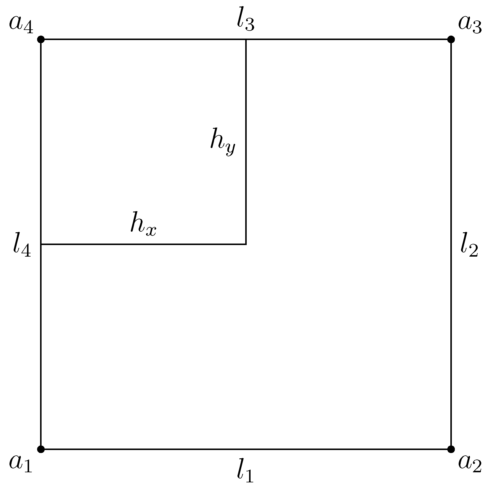
In order to obtain a second-order accuracy estimate, we adopt the high-accuracy integral technique developed in [32]. We introduce the following error function on an element e (see Figure 3):

$$\begin{array}{c}\hfill F\left(y\right)=\frac{1}{2}[{(y-y_e)}^2-h_y^2],\end{array}$$

(13)

where $(x_e,y_e)$ denotes the barycentric coordinate of element e. One can check that $F^{{}^{″}}\left(y\right)=1$, ${F\left(y\right)|}_{l_1,l_3}=0$. Note that v is constant on an element e, and we have

$$\begin{array}{cc}\hfill {({(u-I_{h}u)}_x,v)}_e& ={\int }_e{(u-I_{h}u)}_{x}vdxdy=v{\int }_e{(u-I_{h}u)}_{x}dxdy=v{\int }_e{(u-I_{h}u)}_x{F}^{{}^{″}}\left(y\right)dxdy\hfill \\ \hfill & =v\left[\left({\int }_{l_3}-{\int }_{l_1}\right){(u-I_{h}u)}_x{F}^{{}^{\prime }}\left(y\right)dx-{\int }_e{(u-I_{h}u)}_{xy}{F}^{{}^{\prime }}\left(y\right)dxdy\right]\hfill \\ \hfill & =-\left[\left({\int }_{l_3}-{\int }_{l_1}\right){(u-I_{h}u)}_{xy}F\left(y\right)dx-{\int }_e{(u-I_{h}u)}_{xyy}F\left(y\right)dxdy\right]\hfill \\ \hfill & ={\int }_{e}F\left(y\right)u_{xyy}vdxdy\le C{h}_e^2{\parallel u\parallel }_{3,e}{\parallel v\parallel }_{0,e},\hfill \end{array}$$

(14)

where we have that $(u-I_{h}u)\left(a_i\right)=0$, $(i=1,\dots ,4)$ and $F^{{}^{\prime }}{\left(y\right)|}_{l_1,l_3}$ are constants in the above estimate.

Figure 3. The element $\tilde{e}$.

In the same way, we also have

$$\begin{array}{cc}\hfill {({(u-I_{h}u)}_x,v)}_e& \le C{h}_e^2{\parallel u\parallel }_{3,e}{\parallel v\parallel }_{0,e}.\hfill \end{array}$$

(15)

Therefore, by adding (14) and (15), the desired result (11) is derived. Furthermore, summing up (11) with respect to $e\in {\mathcal{T}}_h$ gives the result (12). □

We present the discrete Gronwall’s inequality, which is useful in the following error analysis.

Lemma 3

([33,34]). Let τ, B and $a_k$, $b_k$, $c_k$, ${\gamma }_k$, for integers $k\ge 0$, be non-negative numbers such that

$$\begin{array}{c}\hfill a_n+\tau \sum _{k=0}^n{b}_k\le \tau \sum _{k=0}^n{\gamma }_k{a}_k+\tau \sum _{k=0}^n{c}_k+B,\mathrm{for}n\ge 0,\end{array}$$

suppose that $\tau {\gamma }_k<1$, for all k, and set ${\sigma }_k={(1-\tau {\gamma }_k)}^{-1}$. Then

$$\begin{array}{c}\hfill a_n+\tau \sum _{k=0}^n{b}_k\le \exp \left(\tau \sum _{k=0}^n{\gamma }_k{\sigma }_k\right)\left(\tau \sum _{k=0}^n{c}_k+B\right),\mathrm{for}n\ge 0.\end{array}$$

The Young inequality will be frequently used in the following analysis, and we present it here.

$$\begin{array}{c}\hfill ab\le \frac{a^2}{2ϵ}+\frac{ϵb^2}{2},\mathrm{f}\mathrm{o}\mathrm{r}ϵ>0.\end{array}$$

The weak formulation of (1)–(4) is as follows: find $(\mathit{u},p):[0,T]\to {\left(H_0^1\left(\mathsf{\Omega }\right)\right)}^2\times L_0^2\left(\mathsf{\Omega }\right)$, such that

$$\begin{array}{cc}\hfill ({\mathit{u}}_t,\mathit{v})+(\nabla \mathit{u},\nabla \mathit{v})+((\mathit{u}·\nabla )\mathit{u},\mathit{v})-(p,\nabla ·\mathit{v})& =(\mathit{f},\mathit{v}),\forall \mathit{v}\in {\left(H_0^1\left(\mathsf{\Omega }\right)\right)}^2,\hfill \end{array}$$

(16)

$$\begin{array}{cc}\hfill (\nabla ·\mathit{u},q)& =0,\forall q\in L_0^2\left(\mathsf{\Omega }\right).\hfill \end{array}$$

(17)

Moreover, in order to give the fully discrete scheme, let $0=t_0<t_1<\cdots <t_N=T$ be a given uniform partition of the time interval with time step $\tau =T/N$ and $t_n=n\tau$, $n=0,1,\dots ,N$. For a smooth function w defined on $[0,T]$, denote

$$\begin{array}{c}\hfill w^n=w\left(t_n\right),D_{\tau }{w}^n=\frac{(w^n-w^{n-1})}{\tau }.\end{array}$$

Then, the semi-implicit backward Euler low-order conforming mixed finite element scheme (bilinear-constant scheme) is as follows: for given $({\mathit{u}}_h^{n-1},p_h^{n-1})\in {\mathit{V}}_h\times M_h$, find $({\mathit{u}}_h^n,p_h^n)\in {\mathit{V}}_h\times M_h$ such that

$$\begin{array}{cc}\hfill (D_{\tau }{\mathit{u}}_h^n,{\mathit{v}}_h)+(\nabla {\mathit{u}}_h^n,\nabla {\mathit{v}}_h)+(({\mathit{u}}_h^{n-1}·\nabla ){\mathit{u}}_h^n,{\mathit{v}}_h)-(p_h^n,\nabla ·{\mathit{v}}_h)& =({\mathit{f}}^n,{\mathit{v}}_h),\forall {\mathit{v}}_h\in {\mathit{V}}_h,\hfill \end{array}$$

(18)

$$\begin{array}{cc}\hfill (\nabla ·{\mathit{u}}_h^n,q_h)& =0,\forall q_h\in M_h,\hfill \end{array}$$

(19)

with the initial approximation ${\mathit{u}}_h^0=I_h{\mathit{u}}_0=I_h\mathit{u}\left(0\right)$.

The unconditionally optimal error estimate for scheme (18)–(19) is shown in [20] by using the error splitting technique with the low-order conforming mixed finite element method, specifically, by introducing the following time-discrete system [18,20]:

$$\begin{array}{cc}\hfill D_{\tau }{\mathit{U}}^n-\Delta {\mathit{U}}^n+({\mathit{U}}^{n-1}·\nabla ){\mathit{U}}^n+\nabla P^n& ={\mathit{f}}^n,\hfill \end{array}$$

(20)

$$\begin{array}{cc}\hfill \nabla ·{\mathit{U}}^n& =0,\hfill \end{array}$$

(21)

$$\begin{array}{cc}\hfill {\mathit{U}}^n& =0,\hfill \end{array}$$

(22)

$$\begin{array}{cc}\hfill {\mathit{U}}^0& ={\mathit{u}}_0.\hfill \end{array}$$

(23)

Then, the error between the exact solution and the numerical solution comprises two parts, where one is the temporal error and the other is the spatial error. Therefore, the numerical solution in the $L^{\infty }$-norm can be bounded without any time-step restrictions. Here, we present a lemma to state the $\tau$-independent boundedness of the numerical solution.

Lemma 4

([20]). Suppose that $({\mathit{u}}^n,p^n)$ is the solution of (1)–(4) with suitable regularity and $({\mathit{U}}^n,P^n)$ and $({\mathit{u}}_h^n,p^n)$ are the solutions of (20)–(23) and (18)–(19). Then, there exist positive constants ${\tau }_0$ and $h_0$ such that when $\tau \le {\tau }_0$ and $h\le h_0$, we have the τ-independent boundedness of numerical solutions

$$\begin{array}{c}\hfill \parallel {\mathit{u}}_h^n{\parallel }_{0,\infty }\le K,n=0,1,\dots ,N,\end{array}$$

(24)

where K is a constant, which is not dependent on h, τ and n.

3. Superclose and Superconvergence Error Estimates

In this section, we firstly present the superclose error estimates for the velocity and pressure variables. Then, we give the superconvergence result in terms of the superclose error estimates as well as the interpolation technique.

Theorem 1.

Suppose that $(\mathit{u},p)$ and $({\mathit{u}}_h^n,p_h^n)$ are the solutions of (16)–(19) and $\mathit{u}\in L^{\infty }({\left(H^3\left(\mathsf{\Omega }\right)\right)}^2\cap {\left(H_0^1\left(\mathsf{\Omega }\right)\right)}^2)$, ${\mathit{u}}_t\in L^{\infty }\left({\left(H^3\left(\mathsf{\Omega }\right)\right)}^2\right)$, ${\mathit{u}}_{tt}\in L^2\left({\left(L^2\left(\mathsf{\Omega }\right)\right)}^2\right)$ and $p\in L^{\infty }\left(H^2\left(\mathsf{\Omega }\right)\right)$. Then, we have the following superclose estimates

$$\begin{array}{c}\hfill \parallel \nabla (I_h{\mathit{u}}^n-{\mathit{u}}_h^n){\parallel }_0\le C(h^2+\tau ),\tau \sum _{k=1}^n{\parallel J_h{p}^n-p_h^n\parallel }_0\le C(h^2+\tau ).\end{array}$$

(25)

Furthermore, we have the following optimal error estimates:

$$\begin{array}{c}\hfill \parallel {\mathit{u}}^n-{\mathit{u}}_h^n{\parallel }_0\le C(h^2+\tau ),\parallel \nabla ({\mathit{u}}^n-{\mathit{u}}_h^n){\parallel }_0\le C(h+\tau ),\tau \sum _{k=1}^n{\parallel p^n-p_h^n\parallel }_0\le C(h+\tau ).\end{array}$$

(26)

Proof. 

For simplicity, we split the errors $\mathit{u}-{\mathit{u}}_h$ and $p-p_h$ as follows:

$$\begin{array}{cc}\hfill & {\mathit{u}}^n-{\mathit{u}}_h^n={\mathit{u}}^n-I_h{\mathit{u}}^n+I_h{\mathit{u}}^n-{\mathit{u}}_h^n:={\mathbf{\rho }}^n+{\mathbf{\theta }}^n,\hfill \\ \hfill & p^n-p_h^n=p^n-J_h{p}^n+J_h{p}^n-p_h^n:={\xi }^n+{\eta }^n.\hfill \end{array}$$

At $t=t_n$, from (16)–(17), we have

$$\begin{array}{cc}\hfill (D_{\tau }{\mathit{u}}^n,{\mathit{v}}_h)+(\nabla {\mathit{u}}^n,\nabla {\mathit{v}}_h)& +(({\mathit{u}}^{n-1}·\nabla ){\mathit{u}}^n,{\mathit{v}}_h)-(\nabla ·{\mathit{v}}_h,p^n)=({\mathit{f}}^n,{\mathit{v}}_h)+(D_{\tau }{\mathit{u}}^n-{\mathit{u}}_t^n,{\mathit{v}}_h)\hfill \\ & +((({\mathit{u}}^{n-1}-{\mathit{u}}^n)·\nabla ){\mathit{u}}^n,{\mathit{v}}_h),\forall {\mathit{v}}_h\in {\mathit{V}}_h,\hfill \end{array}$$

(27)

$$\begin{array}{cc}\hfill & (\nabla ·{\mathit{u}}^n,q_h)=0,\forall q_h\in M_h.\hfill \end{array}$$

(28)

Subtracting (18)–(19) from (27)–(28) gives the following error equations:

$$\begin{array}{cc}\hfill (D_{\tau }{\mathbf{\theta }}^n,{\mathit{v}}_h)+(\nabla {\mathbf{\theta }}^n,\nabla {\mathit{v}}_h)& -(\nabla ·{\mathit{v}}_h,{\eta }^n)=-(D_{\tau }{\mathbf{\rho }}^n,{\mathit{v}}_h)-(\nabla {\mathbf{\rho }}^n,\nabla {\mathit{v}}_h)+(\nabla ·{\mathit{v}}_h,{\xi }^n)\hfill \\ \hfill & -(({\mathit{u}}^{n-1}·\nabla ){\mathit{u}}^n-({\mathit{u}}_h^{n-1}·\nabla ){\mathit{u}}_h^n,{\mathit{v}}_h)+(D_{\tau }{\mathit{u}}^n-{\mathit{u}}_t^n,{\mathit{v}}_h)\hfill \\ \hfill & +((({\mathit{u}}^{n-1}-{\mathit{u}}^n)·\nabla ){\mathit{u}}^n,{\mathit{v}}_h),\forall {\mathit{v}}_h\in {\mathit{V}}_h,\hfill \end{array}$$

(29)

$$\begin{array}{cc}\hfill (\nabla ·{\mathbf{\theta }}^n,q_h)& =-(\nabla ·{\mathbf{\rho }}^n,q_h),\forall q_h\in M_h.\hfill \end{array}$$

(30)

Alternatively, we have

$$\begin{array}{c}\hfill (\nabla ·D_{\tau }{\mathbf{\theta }}^n,q_h)=-(\nabla ·D_{\tau }{\mathbf{\rho }}^n,q_h),\forall q_h\in M_h.\end{array}$$

(31)

Taking ${\mathit{v}}_h=D_{\tau }{\mathbf{\theta }}^n$ in (29) and $q_h={\eta }^n$ in (31) yields that

$$\begin{array}{cc}\hfill \parallel D_{\tau }{\mathbf{\theta }}^n{\parallel }_0^2& +\frac{1}{2\tau }(\parallel \nabla {\mathbf{\theta }}^n{\parallel }_0^2-\parallel \nabla {\mathbf{\theta }}^{n-1}{\parallel }_0^2+\parallel \nabla ({\mathbf{\theta }}^n-{\mathbf{\theta }}^{n-1}){\parallel }_0^2)=-(D_{\tau }{\mathbf{\rho }}^n,D_{\tau }{\mathbf{\theta }}^n)\hfill \\ \hfill & -(\nabla {\mathbf{\rho }}^n,\nabla D_{\tau }{\mathbf{\theta }}^n)+({\xi }^n,\nabla ·D_{\tau }{\mathbf{\theta }}^n)-(\nabla ·D_{\tau }{\mathbf{\rho }}^n,{\eta }^n)\hfill \\ \hfill & -(({\mathit{u}}^{n-1}·\nabla ){\mathit{u}}^n-({\mathit{u}}_h^{n-1}·\nabla ){\mathit{u}}_h^n,D_{\tau }{\mathbf{\theta }}^n)\hfill \\ \hfill & +(D_{\tau }{\mathit{u}}^n-{\mathit{u}}_t^n,D_{\tau }{\mathbf{\theta }}^n)+((({\mathit{u}}^{n-1}-{\mathit{u}}^n)·\nabla ){\mathit{u}}^n,D_{\tau }{\mathbf{\theta }}^n):=\sum _{k=1}^7{E}_k.\hfill \end{array}$$

(32)

Now, we start to estimate $E_k$, $(k=1,\cdots ,7)$ term by term. By the Cauchy–Schwarz inequality and interpolation theory, we have

$$\begin{array}{cc}\hfill E_1& =-(D_{\tau }{\mathbf{\rho }}^n,D_{\tau }{\mathbf{\theta }}^n)\le C{h}^2\parallel {\mathit{u}}_t{\parallel }_{L^{\infty }\left({\left(H^2\left(\mathsf{\Omega }\right)\right)}^2\right)}{\parallel D_{\tau }{\mathbf{\theta }}^n\parallel }_0\hfill \\ \hfill & \le C{h}^2\parallel D_{\tau }{\mathbf{\theta }}^n{\parallel }_0\le C{h}^4+ϵ{\parallel D_{\tau }{\mathbf{\theta }}^n\parallel }_0^2.\hfill \end{array}$$

(33)

Applying the following equality

$$\begin{array}{c}\hfill (a^n,D_{\tau }{b}^n)=D_{\tau }(a^n,b^n)-(D_{\tau }{a}^n,b^{n-1}),\end{array}$$

(34)

we have

$$\begin{array}{cc}\hfill E_2& =-(\nabla {\mathbf{\rho }}^n,\nabla D_{\tau }{\mathbf{\theta }}^n)=-D_{\tau }(\nabla {\mathbf{\rho }}^n,\nabla {\mathbf{\theta }}^n)+(\nabla D_{\tau }{\mathbf{\rho }}^n,\nabla {\mathbf{\theta }}^{n-1})\hfill \\ \hfill & \le -D_{\tau }(\nabla {\mathbf{\rho }}^n,\nabla {\mathbf{\theta }}^n)+C{h}^2\parallel {\mathit{u}}_t{\parallel }_{L^{\infty }{\left(H^3\left(\mathsf{\Omega }\right)\right)}^2}{\parallel \nabla {\mathbf{\theta }}^{n-1}\parallel }_0\hfill \\ \hfill & \le -D_{\tau }(\nabla {\mathbf{\rho }}^n,\nabla {\mathbf{\theta }}^n)+C{h}^4+C{\parallel \nabla {\mathbf{\theta }}^{n-1}\parallel }_0^2,\hfill \end{array}$$

(35)

where we used (8) of Lemma 1 in the above estimate.

With an application of (34) again, it follows that

$$\begin{array}{cc}\hfill E_3& =({\xi }^n,\nabla ·D_{\tau }{\mathbf{\theta }}^n)=D_{\tau }({\xi }^n,\nabla ·{\mathbf{\theta }}^n)-(D_{\tau }{\xi }^n,\nabla ·{\mathbf{\theta }}^{n-1})\hfill \\ \hfill & \le D_{\tau }({\xi }^n,\nabla ·{\mathbf{\theta }}^n)+C{h}^2\parallel p_t{\parallel }_{L^{\infty }\left(H^2\left(\mathsf{\Omega }\right)\right)}{\parallel \nabla {\mathbf{\theta }}^{n-1}\parallel }_0\hfill \\ \hfill & \le D_{\tau }({\xi }^n,\nabla ·{\mathbf{\theta }}^n)+C{h}^4+C{\parallel \nabla {\mathbf{\theta }}^{n-1}\parallel }_0^2,\hfill \end{array}$$

(36)

where we used (9) of Lemma 1 in the above estimate.

According to (10) of Lemma 1, $E_4$ can be bounded by

$$\begin{array}{cc}\hfill E_4& =-(\nabla ·D_{\tau }{\mathbf{\rho }}^n,{\eta }^n)\le C{h}^2\parallel {\mathit{u}}_t{\parallel }_{L^{\infty }{\left(H^3\left(\mathsf{\Omega }\right)\right)}^2}\parallel {\eta }^n{\parallel }_0\le C{h}^2{\parallel {\eta }^n\parallel }_0.\hfill \end{array}$$

(37)

To bound $E_5$, we split $({\mathit{u}}^{n-1}·\nabla ){\mathit{u}}^n-({\mathit{u}}_h^{n-1}·\nabla ){\mathit{u}}_h^n$ as follows:

$$\begin{array}{cc}\hfill ({\mathit{u}}^{n-1}·\nabla ){\mathit{u}}^n& -({\mathit{u}}_h^{n-1}·\nabla ){\mathit{u}}_h^n=(({\mathit{u}}^{n-1}-{\mathit{u}}_h^{n-1})·\nabla ){\mathit{u}}^n+({\mathit{u}}_h^{n-1}·\nabla )({\mathit{u}}^n-{\mathit{u}}_h^n)\hfill \\ \hfill & =(({\mathit{u}}^{n-1}-I_h{\mathit{u}}^{n-1})·\nabla ){\mathit{u}}^n+((I_h{\mathit{u}}^{n-1}-{\mathit{u}}_h^{n-1})·\nabla ){\mathit{u}}^n\hfill \\ \hfill & +({\mathit{u}}_h^{n-1}·\nabla )({\mathit{u}}^n-I_h{\mathit{u}}^n)+({\mathit{u}}_h^{n-1}·\nabla )(I_h{\mathit{u}}^n-{\mathit{u}}_h^n)\hfill \\ \hfill & =(({\mathit{u}}^{n-1}-I_h{\mathit{u}}^{n-1})·\nabla ){\mathit{u}}^n+((I_h{\mathit{u}}^{n-1}-{\mathit{u}}_h^{n-1})·\nabla ){\mathit{u}}^n\hfill \\ \hfill & +(({\mathit{u}}_h^{n-1}-I_h{\mathit{u}}^{n-1})·\nabla )({\mathit{u}}^n-I_h{\mathit{u}}^n)+((I_h{\mathit{u}}^{n-1}-{\mathit{u}}^{n-1})·\nabla )({\mathit{u}}^n-I_h{\mathit{u}}^n)\hfill \\ \hfill & +({\mathit{u}}^{n-1}·\nabla )({\mathit{u}}^n-I_h{\mathit{u}}^n)+({\mathit{u}}_h^{n-1}·\nabla )(I_h{\mathit{u}}^n-{\mathit{u}}_h^n):=\sum _{k=1}^6{F}_k.\hfill \end{array}$$

(38)

In terms of the Cauchy–Schwarz inequality and interpolation theory, we have

$$\begin{array}{cc}\hfill -(F_1,D_{\tau }{\mathbf{\theta }}^n)-(F_2,D_{\tau }{\mathbf{\theta }}^n)& \le (\parallel {\mathbf{\rho }}^{n-1}{\parallel }_0+\parallel {\mathbf{\theta }}^{n-1}{\parallel }_0)\parallel \nabla {\mathit{u}}^n{\parallel }_{0,\infty }{\parallel D_{\tau }{\mathbf{\theta }}^n\parallel }_0\hfill \\ \hfill & \le C(h^2+\parallel \nabla {\mathbf{\theta }}^{n-1}{\parallel }_0)\parallel D_{\tau }{\mathbf{\theta }}^n{\parallel }_0\hfill \\ \hfill & \le C{h}^4+C\parallel \nabla {\mathbf{\theta }}^{n-1}{\parallel }_0^2+2ϵ{\parallel D_{\tau }{\mathbf{\theta }}^n\parallel }_0^2.\hfill \end{array}$$

(39)

Using inverse inequality and interpolation theory, we have

$$\begin{array}{cc}\hfill -(F_3,D_{\tau }{\mathbf{\theta }}^n)-(F_4,D_{\tau }{\mathbf{\theta }}^n)& \le (\parallel {\mathbf{\theta }}^{n-1}{\parallel }_0+\parallel {\mathbf{\rho }}^{n-1}{\parallel }_0)\parallel \nabla {\mathbf{\rho }}^n{\parallel }_0{\parallel D_{\tau }{\mathbf{\theta }}^n\parallel }_{0,\infty }\hfill \\ \hfill & \le C(\parallel \nabla {\mathbf{\theta }}^{n-1}{\parallel }_0+h^2\parallel {\mathit{u}}^{n-1}{\parallel }_2\left)\right(Ch\parallel {\mathit{u}}^n{\parallel }_2\left)\right(C{h}^{-1}\parallel D_{\tau }{\mathbf{\theta }}^n{\parallel }_0)\hfill \\ \hfill & \le C(h^2+\parallel \nabla {\mathbf{\theta }}^{n-1}{\parallel }_0)\parallel D_{\tau }{\mathbf{\theta }}^n{\parallel }_0\hfill \\ \hfill & \le C{h}^4+C\parallel \nabla {\mathbf{\theta }}^{n-1}{\parallel }_0^2+2ϵ{\parallel D_{\tau }{\mathbf{\theta }}^n\parallel }_0^2.\hfill \end{array}$$

(40)

With the aid of (35), one can check that

$$\begin{array}{cc}\hfill -(F_5,D_{\tau }{\mathbf{\theta }}^n)& =-(({\mathit{u}}^{n-1}·\nabla ){\mathbf{\rho }}^n,D_{\tau }{\mathbf{\theta }}^n)=-D_{\tau }(({\mathit{u}}^{n-1}·\nabla ){\mathbf{\rho }}^n,{\mathbf{\theta }}^n)+(D_{\tau }\left(({\mathit{u}}^{n-1}·\nabla ){\mathbf{\rho }}^n\right),{\mathbf{\theta }}^{n-1})\hfill \\ \hfill & =-D_{\tau }(({\mathit{u}}^{n-1}·\nabla ){\mathbf{\rho }}^n,{\mathbf{\theta }}^n)+((D_{\tau }{\mathit{u}}^{n-1}·\nabla ){\mathbf{\rho }}^n,{\mathbf{\theta }}^{n-1})+(({\mathit{u}}^{n-2}·\nabla )D_{\tau }{\mathbf{\rho }}^n,{\mathbf{\theta }}^{n-1}).\hfill \end{array}$$

(41)

In order to obtain a high-accuracy error estimate, i.e., second-order accuracy, we introduce the local $L^2$-projection defined as follows:

$$\begin{array}{c}\hfill {\mathcal{P}}_{e}u=\frac{1}{\left|e\right|}{\int }_{e}udxdy,\end{array}$$

(42)

where e is an element of the partition of ${\mathcal{T}}_h$ and $\left|e\right|$ is the measure of e. Then, we have

$$\begin{array}{c}\hfill \parallel {\mathcal{P}}_e{u\parallel }_{0,e}\le {\parallel u\parallel }_{0,e},\parallel u-{\mathcal{P}}_e{u\parallel }_{0,e}\le C{h}_e{\parallel u\parallel }_{1,e},\parallel u-{\mathcal{P}}_e{u\parallel }_{0,\infty ,e}\le C{h}_e{\parallel u\parallel }_{1,\infty ,e}.\end{array}$$

(43)

Therefore, we have

$$\begin{array}{cc}\hfill ((D_{\tau }{\mathit{u}}^{n-1}·\nabla ){\mathbf{\rho }}^n,{\mathbf{\theta }}^{n-1})& =\sum _{e\in {\mathcal{T}}_h}{((D_{\tau }{\mathit{u}}^{n-1}·\nabla ){\mathbf{\rho }}^n,{\mathbf{\theta }}^{n-1})}_e\hfill \\ \hfill & =\sum _{e\in {\mathcal{T}}_h}\left(((D_{\tau }{\mathit{u}}^{n-1}-{\mathcal{P}}_e{D}_{\tau }{\mathit{u}}^{n-1})·\nabla )\right){\mathbf{\rho }}^n,{\mathbf{\theta }}^{n-1}{)}_e\hfill \\ \hfill & +\sum _{e\in {\mathcal{T}}_h}\left(({\mathcal{P}}_e{D}_{\tau }{\mathit{u}}^{n-1}·\nabla )\right){\mathbf{\rho }}^n,{\mathbf{\theta }}^{n-1}-{\mathcal{P}}_e{\mathbf{\theta }}^{n-1}{)}_e\hfill \\ \hfill & +\sum _{e\in {\mathcal{T}}_h}\left(({\mathcal{P}}_e{D}_{\tau }{\mathit{u}}^{n-1}·\nabla )\right){\mathbf{\rho }}^n,{\mathcal{P}}_e{\mathbf{\theta }}^{n-1}{)}_e\hfill \\ \hfill & \le \sum _{e\in {\mathcal{T}}_h}\parallel D_{\tau }{\mathit{u}}^{n-1}-{\mathcal{P}}_e{D}_{\tau }{\mathit{u}}^{n-1}{\parallel }_{0,\infty ,e}\parallel \nabla {\mathbf{\rho }}^n{\parallel }_{0,e}{\parallel {\mathbf{\theta }}^{n-1}\parallel }_{0,e}\hfill \\ \hfill & +C\sum _{e\in {\mathcal{T}}_h}\parallel \nabla {\mathbf{\rho }}^n{\parallel }_{0,e}\parallel {\mathbf{\theta }}^{n-1}-{\mathcal{P}}_e{\mathbf{\theta }}^{n-1}{\parallel }_{0,e}+C{h}^2\sum _{e\in {\mathcal{T}}_h}\parallel {\mathit{u}}^n{\parallel }_{3,e}{\parallel {\mathcal{P}}_e{\mathbf{\theta }}^{n-1}\parallel }_{0,e}\hfill \\ \hfill & \le C{h}^2\sum _{e\in {\mathcal{T}}_h}\parallel {\mathit{u}}^n{\parallel }_{2,e}\parallel {\mathbf{\theta }}^{n-1}{\parallel }_{0,e}+C{h}^2\sum _{e\in {\mathcal{T}}_h}\parallel {\mathit{u}}^n{\parallel }_{2,e}{\parallel {\mathbf{\theta }}^{n-1}\parallel }_{1,e}\hfill \\ \hfill & +C{h}^2\sum _{e\in {\mathcal{T}}_h}\parallel {\mathit{u}}^n{\parallel }_{3,e}\parallel {\mathbf{\theta }}^{n-1}{\parallel }_{0,e}\le C{h}^2\parallel {\mathit{u}}^n{\parallel }_3\parallel {\mathbf{\theta }}^{n-1}{\parallel }_1\le C{h}^2\parallel {\mathit{u}}^n{\parallel }_3{\parallel \nabla {\mathbf{\theta }}^{n-1}\parallel }_0\hfill \\ \hfill & \le C{h}^4+C{\parallel \nabla {\mathbf{\theta }}^{n-1}\parallel }_0^2,\hfill \end{array}$$

(44)

where we used Lemma 2 in the above estimate.

In the same way, we also have

$$\begin{array}{cc}\hfill (({\mathit{u}}^{n-2}·\nabla )D_{\tau }{\mathbf{\rho }}^n,{\mathbf{\theta }}^{n-1})& \le C{h}^2\parallel \nabla {\mathbf{\theta }}^{n-1}{\parallel }_0\le C{h}^4+C{\parallel \nabla {\mathbf{\theta }}^{n-1}\parallel }_0^2.\hfill \end{array}$$

(45)

Hence, there holds

$$\begin{array}{cc}\hfill -(F_5,D_{\tau }{\mathbf{\theta }}^n)& =-D_{\tau }(({\mathit{u}}^{n-1}·\nabla ){\mathbf{\rho }}^n,{\mathbf{\theta }}^n)+C{h}^4+C{\parallel \nabla {\mathbf{\theta }}^{n-1}\parallel }_0^2.\hfill \end{array}$$

(46)

By (24) of Lemma 4, the numerical solution ${\mathit{u}}_h^n$ is bounded unconditionally in $L^{\infty }$-norm, and we have

$$\begin{array}{cc}\hfill -(F_6,D_{\tau }{\mathbf{\theta }}^n)& \le \parallel {\mathit{u}}_h^n{\parallel }_{0,\infty }\parallel \nabla {\mathbf{\theta }}^n{\parallel }_0\parallel D_{\tau }{\mathbf{\theta }}^n{\parallel }_0\le C\parallel \nabla {\mathbf{\theta }}^n{\parallel }_0{\parallel D_{\tau }{\mathbf{\theta }}^n\parallel }_0\hfill \\ \hfill & \le C\parallel \nabla {\mathbf{\theta }}^n{\parallel }_0^2+ϵ{\parallel D_{\tau }{\mathbf{\theta }}^n\parallel }_0^2.\hfill \end{array}$$

(47)

Based on the above estimates $(F_k,D_{\tau }{\mathbf{\theta }}^n)$, $(k=1,\dots ,6)$, $E_5$ reduces to

$$\begin{array}{cc}\hfill E_5& \le C{h}^4+C(\parallel \nabla {\mathbf{\theta }}^n{\parallel }_0^2+\parallel \nabla {\mathbf{\theta }}^{n-1}{\parallel }_0^2)+5ϵ\parallel D_{\tau }{\mathbf{\theta }}^n{\parallel }_0^2-D_{\tau }(({\mathit{u}}^{n-1}·\nabla ){\mathbf{\rho }}^n,{\mathbf{\theta }}^n).\hfill \end{array}$$

(48)

Moreover, by Taylor expansion, we have

$$\begin{array}{cc}\hfill E_6+E_7& \le C\tau \parallel {\mathit{u}}_{tt}{\parallel }_{L^{\infty }\left(L^2\left(\mathsf{\Omega }\right)\right)}\parallel D_{\tau }{\mathbf{\theta }}^n{\parallel }_0+C\tau \parallel {\mathit{u}}_t{\parallel }_{L^{\infty }\left(L^2\left(\mathsf{\Omega }\right)\right)}{\parallel \nabla \mathit{u}\parallel }_{L^{\infty }\left(L^{\infty }\left(\mathsf{\Omega }\right)\right)}{\parallel D_{\tau }{\mathbf{\theta }}^n\parallel }_0\hfill \\ \hfill & \le C\tau \parallel D_{\tau }{\mathbf{\theta }}^n{\parallel }_0\le C{\tau }^2+ϵ{\parallel D_{\tau }{\mathbf{\theta }}^n\parallel }_0^2.\hfill \end{array}$$

(49)

With the estimates $E_k$, $(k=1,\dots ,6)$, we obtain

$$\begin{array}{cc}\hfill \parallel D_{\tau }{\mathbf{\theta }}^n{\parallel }_0^2+\frac{1}{2\tau }(\parallel \nabla {\mathbf{\theta }}^n{\parallel }_0^2-\parallel \nabla {\mathbf{\theta }}^{n-1}{\parallel }_0^2)& \le C(h^4+{\tau }^2)+C(\parallel \nabla {\mathbf{\theta }}^n{\parallel }_0^2+\parallel \nabla {\mathbf{\theta }}^{n-1}{\parallel }_0^2)\hfill \\ \hfill & +7ϵ\parallel D_{\tau }{\mathbf{\theta }}^n{\parallel }_0^2+C{h}^2{\parallel {\eta }^n\parallel }_0-D_{\tau }(\nabla {\mathbf{\rho }}^n,\nabla {\mathbf{\theta }}^n)\hfill \\ \hfill & +D_{\tau }({\xi }^n,\nabla ·{\mathbf{\theta }}^n)-D_{\tau }(({\mathit{u}}^{n-1}·\nabla ){\mathbf{\rho }}^n,{\mathbf{\theta }}^n).\hfill \end{array}$$

(50)

On the other hand, from (29), it follows that

$$\begin{array}{cc}\hfill (\nabla ·{\mathit{v}}_h,{\eta }^n)& =(D_{\tau }{\mathbf{\theta }}^n,{\mathit{v}}_h)+(D_{\tau }{\mathbf{\rho }}^n,{\mathit{v}}_h)+(\nabla {\mathbf{\theta }}^n,\nabla {\mathit{v}}_h)+(\nabla {\mathbf{\rho }}^n,\nabla {\mathit{v}}_h)-(\nabla ·{\mathit{v}}_h,{\xi }^n)\hfill \\ \hfill & +(({\mathit{u}}^{n-1}·\nabla ){\mathit{u}}^n-({\mathit{u}}_h^{n-1}·\nabla ){\mathit{u}}_h^n,{\mathit{v}}_h)-(D_{\tau }{\mathit{u}}^n-{\mathit{u}}_t^n,{\mathit{v}}_h)\hfill \\ \hfill & -((({\mathit{u}}^{n-1}-{\mathit{u}}^n)·\nabla ){\mathit{u}}^n,{\mathit{v}}_h),\forall {\mathit{v}}_h\in {\mathit{V}}_h.\hfill \end{array}$$

(51)

Then, one can check that by the Cauchy–Schwarz inequality and interpolation theory,

$$\begin{array}{cc}\hfill (D_{\tau }{\mathbf{\theta }}^n,{\mathit{v}}_h)+(D_{\tau }{\mathbf{\rho }}^n,{\mathit{v}}_h)& \le (\parallel D_{\tau }{\mathbf{\theta }}^n{\parallel }_0+\parallel D_{\tau }{\mathbf{\rho }}^n{\parallel }_0)\parallel {\mathit{v}}_h{\parallel }_0\hfill \\ \hfill & \le C(h^2+\parallel D_{\tau }{\mathbf{\theta }}^n{\parallel }_0)\parallel \nabla {\mathit{v}}_h{\parallel }_0\hfill \end{array}$$

(52)

and

$$\begin{array}{cc}\hfill (\nabla {\mathbf{\theta }}^n,\nabla {\mathit{v}}_h)& \le \parallel \nabla {\mathbf{\theta }}^n{\parallel }_0{\parallel \nabla {\mathit{v}}_h\parallel }_0.\hfill \end{array}$$

(53)

By Lemma 1, we have

$$\begin{array}{cc}\hfill (\nabla {\mathbf{\rho }}^n,\nabla {\mathit{v}}_h)-(\nabla ·{\mathit{v}}_h,{\xi }^n)& \le C{h}^2{\parallel \nabla {\mathit{v}}_h\parallel }_0.\hfill \end{array}$$

(54)

Using a similar estimate process as $E_5$, there holds

$$\begin{array}{cc}\hfill (({\mathit{u}}^{n-1}·\nabla ){\mathit{u}}^n-({\mathit{u}}_h^{n-1}·\nabla ){\mathit{u}}_h^n,{\mathit{v}}_h)& \le C(h^2+\parallel \nabla {\mathbf{\theta }}^n{\parallel }_0+\parallel \nabla {\mathbf{\theta }}^{n-1}{\parallel }_0)\parallel \nabla {\mathit{v}}_h{\parallel }_0.\hfill \end{array}$$

(55)

As an application of the Taylor expansion, we have

$$\begin{array}{cc}\hfill -(D_{\tau }{\mathit{u}}^n-{\mathit{u}}_t^n,{\mathit{v}}_h)-((({\mathit{u}}^{n-1}-{\mathit{u}}^n)·\nabla ){\mathit{u}}^n,{\mathit{v}}_h)& \le C\tau \parallel \nabla {\mathit{v}}_h{\parallel }_0.\hfill \end{array}$$

(56)

Therefore, we conclude that

$$\begin{array}{cc}\hfill (\nabla ·{\mathit{v}}_h,{\eta }^n)& \le C(h^2+\tau +\parallel \nabla {\mathbf{\theta }}^n{\parallel }_0+\parallel \nabla {\mathbf{\theta }}^{n-1}{\parallel }_0+\parallel D_{\tau }{\mathbf{\theta }}^n{\parallel }_0)\parallel \nabla {\mathit{v}}_h{\parallel }_0.\hfill \end{array}$$

(57)

Then, thanks to the discrete LBB condition ($\beta$ is a positive constant independent of mesh-size h), we have

$$\begin{array}{c}\hfill \beta \parallel {\eta }^n{\parallel }_0\le \underset{0\ne {\mathit{v}}_h\in {\mathit{V}}_h}{sup}\frac{(\nabla ·{\mathit{v}}_h,{\eta }^n)}{\parallel \nabla {\mathit{v}}_h{\parallel }_0}\le C(h^2+\tau +\parallel \nabla {\mathbf{\theta }}^n{\parallel }_0+\parallel \nabla {\mathbf{\theta }}^{n-1}{\parallel }_0+\parallel D_{\tau }{\mathbf{\theta }}^n{\parallel }_0).\end{array}$$

(58)

Substituting (58) into (50) and using the Young inequality, (50) reduces to

$$\begin{array}{cc}\hfill \parallel D_{\tau }{\mathbf{\theta }}^n{\parallel }_0^2+\frac{1}{2\tau }(\parallel \nabla {\mathbf{\theta }}^n{\parallel }_0^2-\parallel \nabla {\mathbf{\theta }}^{n-1}{\parallel }_0^2)& \le C(h^4+{\tau }^2)+C(\parallel \nabla {\mathbf{\theta }}^n{\parallel }_0^2+\parallel \nabla {\mathbf{\theta }}^{n-1}{\parallel }_0^2)\hfill \\ \hfill & +8ϵ\parallel D_{\tau }{\mathbf{\theta }}^n{\parallel }_0^2-D_{\tau }(\nabla {\mathbf{\rho }}^n,\nabla {\mathbf{\theta }}^n)\hfill \\ \hfill & +D_{\tau }({\xi }^n,\nabla ·{\mathbf{\theta }}^n)-D_{\tau }(({\mathit{u}}^{n-1}·\nabla ){\mathbf{\rho }}^n,{\mathbf{\theta }}^n).\hfill \end{array}$$

(59)

Choosing $ϵ=\frac{1}{16}$ in (59) and summing up the resulting inequality, we have

$$\begin{array}{cc}\hfill \frac{\tau }{2}\sum _{k=1}^n\parallel D_{\tau }{\mathbf{\theta }}^k{\parallel }_0^2+\frac{1}{2}{\parallel \nabla {\mathbf{\theta }}^n\parallel }_0^2& \le C(h^4+{\tau }^2)+C\tau \sum _{k=1}^n{\parallel \nabla {\mathbf{\theta }}^k\parallel }_0^2-(\nabla {\mathbf{\rho }}^n,\nabla {\mathbf{\theta }}^n)\hfill \\ \hfill & +({\xi }^n,\nabla ·{\mathbf{\theta }}^n)-(({\mathit{u}}^{n-1}·\nabla ){\mathbf{\rho }}^n,{\mathbf{\theta }}^n),\hfill \\ \hfill & \le C(h^4+{\tau }^2)+C\tau \sum _{k=1}^n\parallel \nabla {\mathbf{\theta }}^k{\parallel }_0^2+C{h}^2\parallel {\mathit{u}}^n{\parallel }_3{\parallel \nabla {\mathbf{\theta }}^n\parallel }_0\hfill \\ \hfill & +C{h}^2\parallel p^n{\parallel }_3\parallel \nabla {\mathbf{\theta }}^n{\parallel }_0+C{h}^2\parallel {\mathit{u}}^n{\parallel }_3{\parallel \nabla {\mathbf{\theta }}^n\parallel }_0\hfill \\ \hfill & \le C(h^4+{\tau }^2)+C\tau \sum _{k=1}^n\parallel \nabla {\mathbf{\theta }}^k{\parallel }_0^2+\frac{1}{4}{\parallel \nabla {\mathbf{\theta }}^n\parallel }_0^2,\hfill \end{array}$$

(60)

where we used ${\mathbf{\theta }}^0=0$, Lemma 1 and the same estimate process (44) for $-(({\mathit{u}}^{n-1}·\nabla ){\mathbf{\rho }}^n,{\mathbf{\theta }}^n)$.

Hence, from (60), there holds

$$\begin{array}{cc}\hfill \tau \sum _{k=1}^n\parallel D_{\tau }{\mathbf{\theta }}^k{\parallel }_0^2+{\parallel \nabla {\mathbf{\theta }}^n\parallel }_0^2& \le C(h^4+{\tau }^2)+C\tau \sum _{k=1}^n{\parallel \nabla {\mathbf{\theta }}^k\parallel }_0^2.\hfill \end{array}$$

(61)

Then, an application of the Gronwall lemma (see Lemma 3) yields

$$\begin{array}{c}\hfill \tau \sum _{k=1}^n\parallel D_{\tau }{\mathbf{\theta }}^k{\parallel }_0^2+{\parallel \nabla {\mathbf{\theta }}^n\parallel }_0^2\le C(h^4+{\tau }^2).\end{array}$$

(62)

Putting (62) into (58) gives that

$$\begin{array}{cc}\hfill \tau \sum _{k=1}^n{\parallel \eta \parallel }_0& \le C(h^2+\tau )+\tau \sum _{k=1}^n{\parallel D_{\tau }{\mathbf{\theta }}^n\parallel }_0\hfill \\ \hfill & \le C(h^2+\tau )+C{\left(\tau \sum _{k=1}^n{\parallel D_{\tau }{\mathbf{\theta }}^k\parallel }_0^2\right)}^{\frac{1}{2}}\hfill \\ \hfill & \le C(h^2+\tau ).\hfill \end{array}$$

(63)

The desired results are obtained, and the proof is complete. □

With the aid of the superclose error estimate in Theorem 1, we adopt the interpolation post-processing approach to improve the accuracy of the numerical solution $({\mathit{u}}_h^n,p_h^n)$ on the whole domain. Let $I_{2h}$ be the piecewise biquadratic nodal interpolation operator for the velocity associated with ${\mathcal{T}}_{2h}$. Moreover, for the pressure, the postprocessing operator $J_{2h}$ is defined as

$$\left\{\begin{array}{c}{J}_{2h}p\in Q_{11}\left(\tilde{e}\right),\hfill \\ \frac{1}{|e_i|}{\int }_{e_i}(J_{2h}p-p)d{x}_1{x}_2=0,i=1,2,3,4.\hfill \end{array}\right.$$

The following properties are shown in [29]:

$$\left\{\begin{array}{c}{I}_{2h}{I}_h=I_{2h},\hfill \\ \parallel I_{2h}{\mathit{v}\parallel }_1\le C{\parallel \mathit{v}\parallel }_1,\forall \mathit{v}\in {\mathit{V}}_h,\hfill \\ \parallel I_{2h}{\mathit{u}-\mathit{u}\parallel }_1\le C{h}^2{\parallel \mathit{u}\parallel }_3,\hfill \end{array}\right.\left\{\begin{array}{c}{J}_{2h}{J}_h^{{}^{\prime }}=J_{2h},\hfill \\ \parallel J_{2h}{q\parallel }_0\le C{\parallel q\parallel }_0,\forall q\in P_h,\hfill \\ \parallel J_{2h}{p-p\parallel }_0\le C{h}^2{\parallel p\parallel }_2.\hfill \end{array}\right.$$

(64)

Moreover, we also have from [29] that for $p\in H^2\left(\mathsf{\Omega }\right)$,

$$\begin{array}{c}\hfill \parallel p-J_{2h}{J}_h{p\parallel }_0\le C{h}^2{\parallel p\parallel }_2.\end{array}$$

(65)

Now, we state the global superonvergence result in the following theorem:

Theorem 2.

Under the condition of Theorem 1, there holds

$$\begin{array}{c}\hfill \parallel {\mathit{u}}^n-I_{2h}{\mathit{u}}_h^n{\parallel }_1+{\parallel p^n-J_{2h}{p}_h^n\parallel }_0\le C(h^2+\tau ).\end{array}$$

(66)

Proof. 

By (64) and (65), we have

$$\begin{array}{cc}\hfill \parallel {\mathit{u}}^n-I_{2h}{\mathit{u}}_h^n{\parallel }_1+{\parallel p^n-J_{2h}{p}_h^n\parallel }_0& \le \parallel {\mathit{u}}^n-I_{2h}{I}_h{\mathit{u}}^n{\parallel }_1+{\parallel I_{2h}{I}_h{\mathit{u}}^n-I_{2h}{\mathit{u}}_h^n\parallel }_1\hfill \\ \hfill & +\parallel p^n-J_{2h}{J}_h{p}^n{\parallel }_0+{\parallel J_{2h}{J}_h{p}^n-J_{2h}{p}_h^n\parallel }_0\hfill \\ \hfill & \le C{h}^2\parallel {\mathit{u}}^n{\parallel }_3+C\parallel I_h{\mathit{u}}^n-{\mathit{u}}_h^n{\parallel }_1+C{h}^2\parallel p^n{\parallel }_2+C{\parallel J_h{p}^n-p_h^n\parallel }_0\hfill \\ \hfill & \le C(h^2+\tau ).\hfill \end{array}$$

The proof is complete. □

4. Numerical Experiment

In this section, we present some numerical results to confirm the correctness of the theoretical analysis. The software we used is MATLAB 2018a with a 3.20 GHz Intel Core i5-6500 CPU processor and 8 GB memory.

Example 1.

Let $\mathsf{\Omega }={(0,1)}^2$, and divide $\mathsf{\Omega }$ into $m\times n$ uniform rectangles. Moreover, the function $\mathit{f}$ and the initial and boundary conditions are chosen corresponding to the exact solution [35]:

$$\begin{array}{cc}\hfill & u_1=e^{-t}(x_1^4-2x_1^3+x_1^2)(4x_2^3-6x_2^2+2x_2),\hfill \\ \hfill & u_2=-e^{-t}(x_2^4-2x_2^3+x_2^2)(4x_1^3-6x_1^2+2x_1),\hfill \\ \hfill & p=10e^{-t}(2x_1-1)(2x_2-1).\hfill \end{array}$$

We set the final time $T=1.0$ in the computation. In order to confirm the error estimates in Theorems 1 and 2, we present the numerical errors in Table 1, Table 2, Table 3, Table 4, Table 5 and Table 6 at $t=0.1,0.6,1.0$, respectively. Obviously, it can be seen that the numerical results are in agreement with the theoretical analysis, i.e., the errors $\parallel {\mathit{u}}^n-{\mathit{u}}_h^n{\parallel }_0$, $\parallel {\mathit{u}}^n-{\mathit{u}}_h^n{\parallel }_1$, $\parallel I_h{\mathit{u}}^n-{\mathit{u}}_h^n{\parallel }_1$ and $\parallel {\mathit{u}}^n-I_{2h}{\mathit{u}}_h^n{\parallel }_1$ for the velocity $\mathit{u}$ are of order $O\left(h^2\right)$, $O\left(h\right)$, $O\left(h^2\right)$ and $O\left(h^2\right)$, respectively. 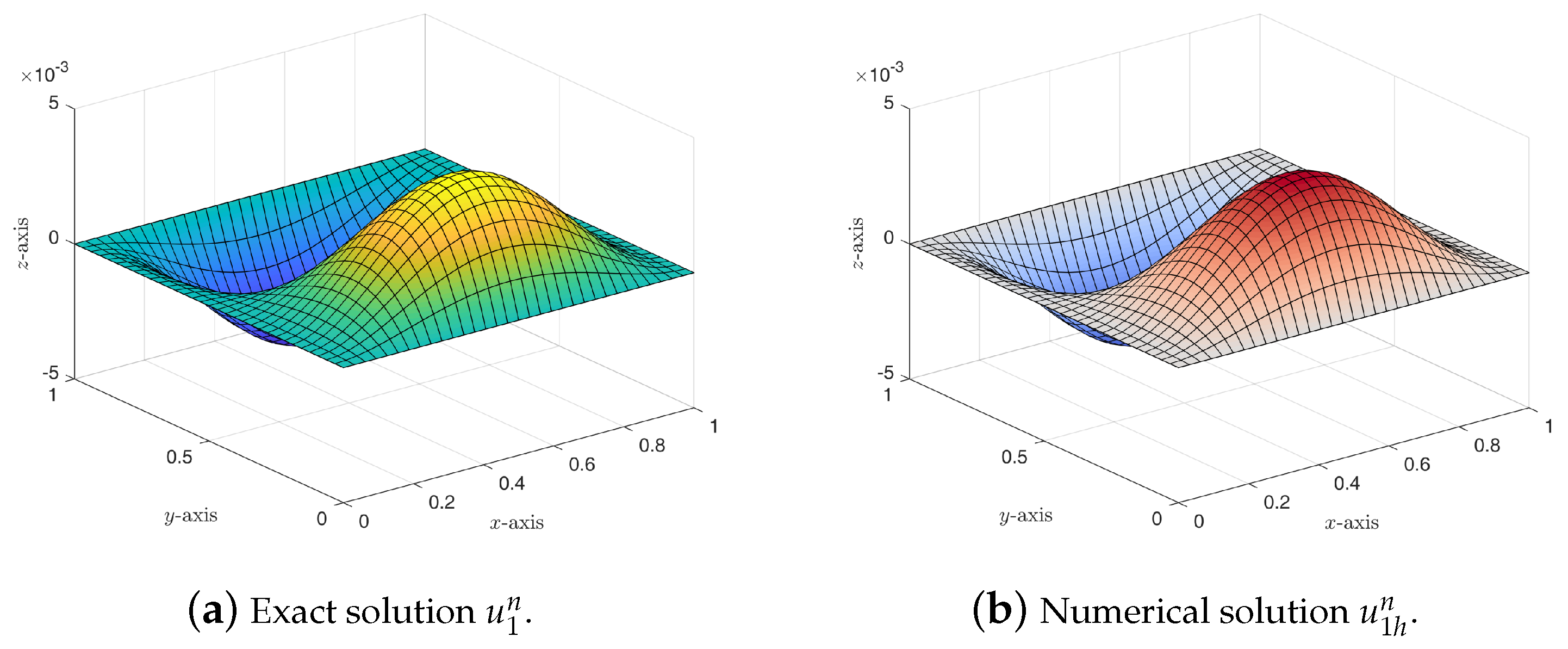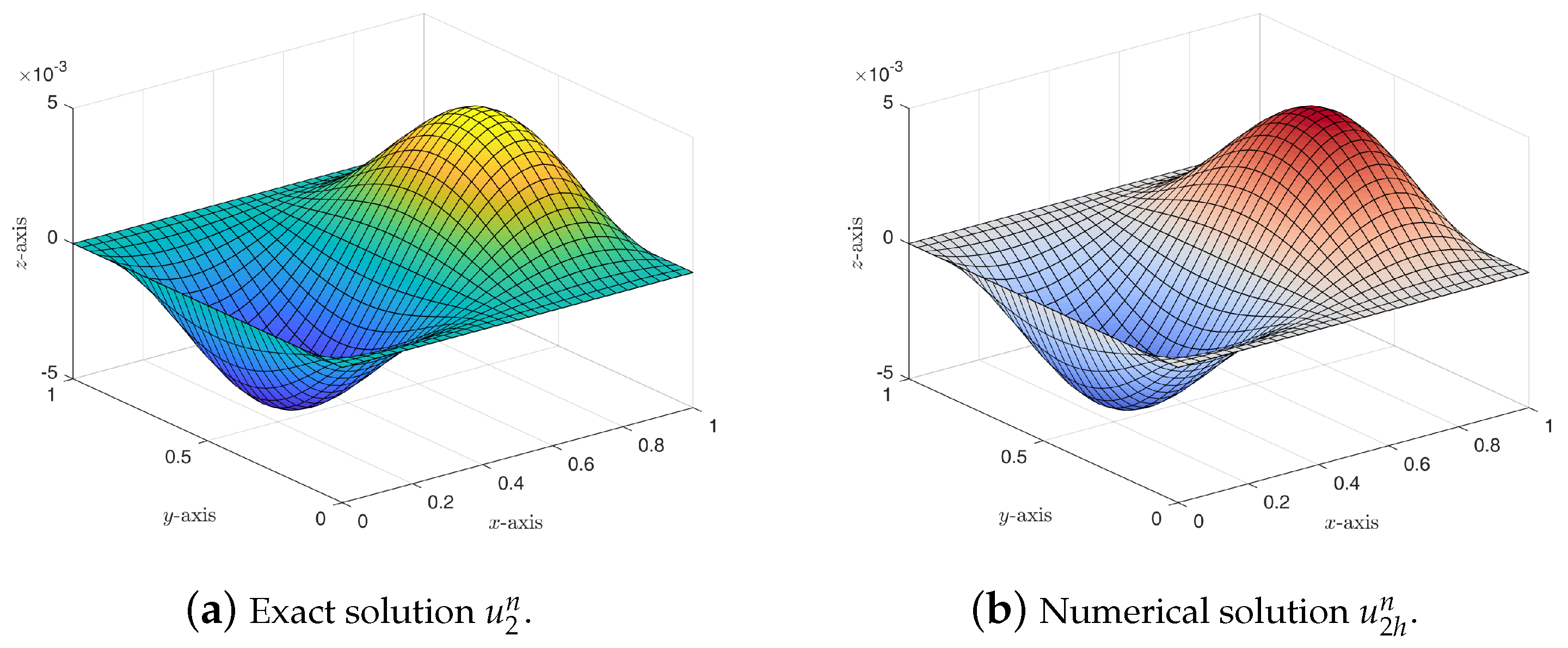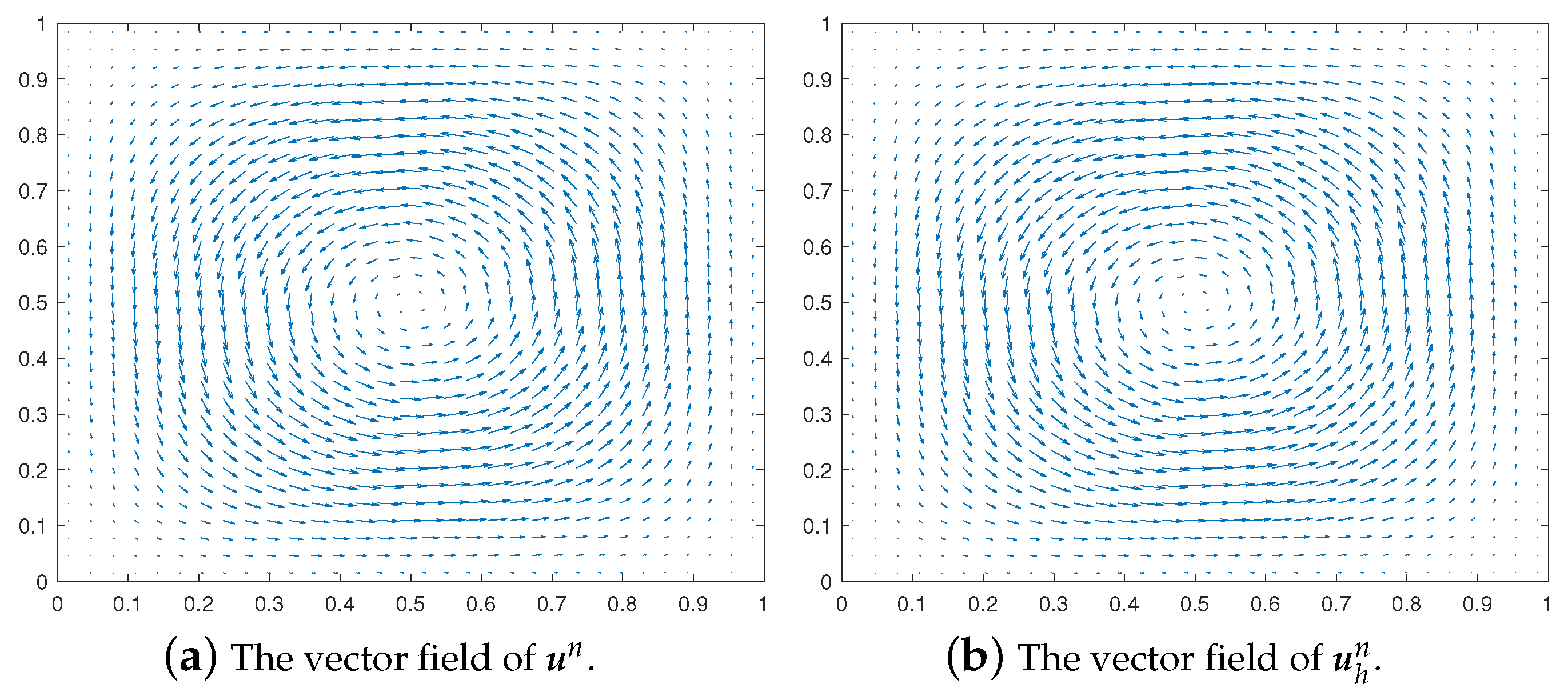In addition, the errors $\parallel p^n-p_h^n{\parallel }_0$, $\parallel J_h{p}^n-p_h^n{\parallel }_0$ and $\parallel p^n-J_{2h}{p}_h^n{\parallel }_0$ for the pressure p are of orders $O\left(h\right)$, $O\left(h^2\right)$ and $O\left(h^2\right)$, respectively. At the same time, we also give the graphics of the exact solutions ($\mathit{u},p$) and finite element solutions (${\mathit{u}}_h,p_h$) at $t=1.0$ on mesh $32\times 32$ (see Figure 4, Figure 5, Figure 6 and Figure 7), respectively. It can be seen that the numerical results are also in good agreement with the theoretical analysis.

Example 2.

Let $\mathsf{\Omega }={(0,1)}^2$ and divide $\mathsf{\Omega }$ into $m\times n$ uniform rectangles. Moreover, the function $\mathit{f}$ and the initial and boundary conditions are chosen corresponding to the exact solution [14]:

$$\begin{array}{cc}\hfill & u_1=-e^{-2t}{sin}^2\left(\pi x\right)sin\left(\pi y\right)cos\left(\pi y\right),\hfill \\ \hfill & u_2=e^{-2t}sin\left(\pi x\right)cos\left(\pi x\right){sin}^2\left(\pi y\right),\hfill \\ \hfill & p=e^{-4t}sin\left(\pi x\right)sin\left(\pi y\right).\hfill \end{array}$$

Table 1. The numerical errors and convergence orders at $t=0.1$ of $\mathit{u}$.

$\mathit{m}\times \mathit{n}$	$4\times 4$	$8\times 8$	$16\times 16$	$32\times 32$
$\parallel {\mathit{u}}^n-{\mathit{u}}_h^n{\parallel }_0$	6.9832 × 10${}^{-4}$	1.7443 × 10${}^{-4}$	4.0642 × 10${}^{-5}$	1.0779 × 10${}^{-5}$
Order	/	2.0012	2.1016	1.9147
$\parallel {\mathit{u}}^n-{\mathit{u}}_h^n{\parallel }_1$	2.7565 × 10${}^{-2}$	1.3929 × 10${}^{-2}$	6.9778 × 10${}^{-3}$	3.4900 × 10${}^{-3}$
Order	/	0.98469	0.99730	0.99953
$\parallel I_h{\mathit{u}}^n-{\mathit{u}}_h^n{\parallel }_1$	5.1545 × 10${}^{-3}$	1.7229 × 10${}^{-3}$	4.9365 × 10${}^{-4}$	1.1691 × 10${}^{-4}$
Order	/	1.5810	1.8033	2.0780
$\parallel {\mathit{u}}^n-I_{2h}{\mathit{u}}_h^n{\parallel }_1$	1.6546 × 10${}^{-2}$	4.4691 × 10${}^{-3}$	1.1290 × 10${}^{-3}$	2.7815 × 10${}^{-4}$
Order	/	1.8884	1.9849	2.0211

Table 2. The numerical errors and convergence orders at $t=0.1$ of p.

$\mathit{m}\times \mathit{n}$	$8\times 8$	$16\times 16$	$32\times 32$	$64\times 64$
$\parallel p-p_h{\parallel }_0$	1.1969×10${}^{+0}$	5.4990×10${}^{-1}$	2.6876×10${}^{-1}$	1.3356×10${}^{-1}$
Order	/	1.1221	1.0329	1.0088
$\parallel J_{h}p-p_h{\parallel }_0$	5.7535×10${}^{-1}$	1.4260×10${}^{-1}$	3.6042×10${}^{-2}$	8.9144×10${}^{-3}$
Order	/	2.0125	1.9842	2.0154
$\parallel p-J_{2h}{p}_h{\parallel }_0$	7.6225×10${}^{-1}$	1.8945×10${}^{-1}$	4.7655×10${}^{-2}$	1.1841×10${}^{-2}$
Order	/	2.0084	1.9911	2.0089

Table 3. The numerical errors and convergence orders at $t=0.6$ of $\mathit{u}$.

$\mathit{m}\times \mathit{n}$	$4\times 4$	$8\times 8$	$16\times 16$	$32\times 32$
$\parallel {\mathit{u}}^n-{\mathit{u}}_h^n{\parallel }_0$	2.4270×10${}^{-4}$	6.3566×10${}^{-5}$	1.4898×10${}^{-5}$	3.9554×10${}^{-6}$
Order	/	1.9329	2.0931	1.9132
$\parallel {\mathit{u}}^n-{\mathit{u}}_h^n{\parallel }_1$	1.6737×10${}^{-}$	8.4489×10${}^{-3}$	4.2323×10${}^{-3}$	2.1168×10${}^{-3}$
Order	/	0.98623	0.99734	0.99953
$\parallel I_h{\mathit{u}}^n-{\mathit{u}}_h^n{\parallel }_1$	3.5044e×10${}^{-3}$	1.0579×10${}^{-3}$	3.0068×10${}^{-4}$	7.1119×10${}^{-5}$
Order	/	1.7279	1.8149	2.0799
$\parallel {\mathit{u}}^n-I_{2h}{\mathit{u}}_h^n{\parallel }_1$	1.0152×10${}^{-2}$	2.7162×10${}^{-3}$	6.8536×10${}^{-4}$	1.6879×10${}^{-4}$
Order	/	1.9022	1.9867	2.0216

Table 4. The numerical errors and convergence orders at $t=0.6$ of p.

$\mathit{m}\times \mathit{n}$	$8\times 8$	$16\times 16$	$32\times 32$	$64\times 64$
$\parallel p-p_h{\parallel }_0$	7.2597×10${}^{-1}$	3.3353×10${}^{-1}$	1.6301×10${}^{-1}$	8.1008×10${}^{-2}$
Order	/	1.1221	1.0329	1.0088
$\parallel J_{h}p-p_h{\parallel }_0$	3.4897×10${}^{-1}$	8.6491×10${}^{-2}$	2.1860×10${}^{-2}$	5.4069×10${}^{-3}$
Order	/	2.0125	1.9842	2.0154
$\parallel p-J_{2h}{p}_h{\parallel }_0$	4.6233×10${}^{-1}$	1.1491×10${}^{-1}$	2.8905×10${}^{-2}$	7.1817×10${}^{-3}$
Order	/	2.0084	1.9911	2.0089

Table 5. The numerical errors and convergence orders at $t=1.0$ of $\mathit{u}$.

$\mathit{m}\times \mathit{n}$	$4\times 4$	$8\times 8$	$16\times 16$	$32\times 32$
$\parallel {\mathit{u}}^n-{\mathit{u}}_h^n{\parallel }_0$	1.2510×10${}^{-4}$	3.2199×10${}^{-5}$	8.0816×10${}^{-6}$	2.0220×10${}^{-6}$
Order	/	1.9580	1.9943	1.9989
$\parallel {\mathit{u}}^n-{\mathit{u}}_h^n{\parallel }_1$	1.1202×10${}^{-2}$	5.6624×10${}^{-3}$	2.8366×10${}^{-3}$	1.4189×10${}^{-3}$
Order	/	0.98430	0.99724	0.99938
$\parallel I_h{\mathit{u}}^n-{\mathit{u}}_h^n{\parallel }_1$	1.7780×10${}^{-3}$	6.0911×10${}^{-4}$	1.6246×10${}^{-4}$	4.1252×10${}^{-5}$
Order	/	1.5455	1.9066	1.9775
$\parallel {\mathit{u}}^n-I_{2h}{\mathit{u}}_h^n{\parallel }_1$	6.6492×10${}^{-3}$	1.7801×10${}^{-3}$	4.4318×10${}^{-4}$	1.1058×10${}^{-4}$
Order	/	1.9012	2.0060	2.0029

Table 6. The numerical errors and convergence orders at $t=1.0$ of p.

$\mathit{m}\times \mathit{n}$	$8\times 8$	$16\times 16$	$32\times 32$	$64\times 64$
$\parallel p-p_h{\parallel }_0$	4.8472×10${}^{-1}$	2.2345×10${}^{-1}$	1.0923×10${}^{-1}$	5.4300×10${}^{-2}$
Order	/	1.1172	1.0325	1.0084
$\parallel J_{h}p-p_h{\parallel }_0$	2.2993×10${}^{-1}$	5.7482×10${}^{-2}$	1.4370×10${}^{-2}$	3.5926×10${}^{-3}$
Order	/	2.0000	2.0000	2.0000
$\parallel p-J_{2h}{p}_h{\parallel }_0$	3.0657×10${}^{-1}$	7.6642×10${}^{-2}$	1.9160×10${}^{-3}$	4.7901×10${}^{-3}$
Order	/	2.0000	2.0000	2.0000

Figure 4. The graphics of $u_1^n$ and $u_{1h}^n$ on mesh $32\times 32$.

Figure 5. The graphics of $u_2^n$ and $u_{2h}^n$ on mesh $32\times 32$.

Figure 6. The graphics of the vector fields on mesh $32\times 32$.

Figure 7. The graphics of $p^n$ and $p_h^n$ on mesh $32\times 32$.

We set the final time $T=10$ in the computation. In order to confirm the error estimates in Theorems 1 and 2, we present the numerical errors in Table 7 and Table 8 at $t=10$. Obviously, it can be seen that numerical results are in agreement with the theoretical analysis.

Table 7. The numerical errors and convergence orders at $t=10$ of $\mathit{u}$.

$\mathit{m}\times \mathit{n}$	$4\times 4$	$8\times 8$	$16\times 16$	$32\times 32$
$\parallel {\mathit{u}}^n-{\mathit{u}}_h^n{\parallel }_0$	3.9072×10${}^{-18}$	9.6945×10${}^{-19}$	2.4129×10${}^{-19}$	6.0248×10${}^{-20}$
Order	/	2.0109	2.0064	2.0018
$\parallel {\mathit{u}}^n-{\mathit{u}}_h^n{\parallel }_1$	2.0623×10${}^{-9}$	1.0366×10${}^{-9}$	5.1886×10${}^{-10}$	2.5950×10${}^{-10}$
Order	/	0.99241	0.99839	0.99959
$\parallel I_h{\mathit{u}}^n-{\mathit{u}}_h^n{\parallel }_1$	3.0875×10${}^{-10}$	1.0500×10${}^{-10}$	2.8119×10${}^{-11}$	7.1483×10${}^{-12}$
Order	/	1.5560	1.9008	1.9759
$\parallel {\mathit{u}}^n-I_{2h}{\mathit{u}}_h^n{\parallel }_1$	1.2562×10${}^{-9}$	4.2567×10${}^{-10}$	1.0848×10${}^{-10}$	2.7240×10${}^{-11}$
Order	/	1.5612	1.9723	1.9937

Table 8. The numerical errors and convergence orders at $t=10$ of p.

$\mathit{m}\times \mathit{n}$	$8\times 8$	$16\times 16$	$32\times 32$	$64\times 64$
$\parallel p-p_h{\parallel }_0$	2.4684×10${}^{-10}$	7.9753×10${}^{-11}$	2.0617×10${}^{-11}$	5.1913×10${}^{-12}$
Order	/	1.6300	1.9517	1.9896
$\parallel J_{h}p-p_h{\parallel }_0$	2.4684×10${}^{-10}$	7.9753×10${}^{-11}$	2.0617×10${}^{-11}$	5.1913×10${}^{-12}$
Order	/	1.6300	1.9517	1.9896
$\parallel p-J_{2h}{p}_h{\parallel }_0$	2.8503×10${}^{-10}$	8.7022×10${}^{-11}$	2.1086×10${}^{-11}$	5.2215×10${}^{-12}$
Order	/	1.7117	2.0451	2.0138

5. Conclusions

In this paper, a low-order conforming mixed finite element method is investigated for time-dependent Navier–Stokes equations with the semi-implicit Euler scheme. With the help of the error splitting technique and the high-accuracy error estimates of the element pair on the rectangular mesh, the numerical solution in $L^{infty}$-norm is obtained without any time-step restrictions. Furthermore, the unconditionally superclose error estimates are derived by treating the trilinear term rigorously and skillfully. Moreover, the global superconvergence results are acquired in terms of the interpolation post-processing approach. It should be pointed out there are many interesting topics to study in future works, such as high-order time (e.g., Crank–Nicolson scheme and BDF2 scheme), low-order nonconforming mixed finite element methods, and fast computing for discretized linear system. We will study these topics in the future.