Stability and Neimark–Sacker Bifurcation of a Delay Difference Equation

Abstract

In this paper, we revisit a delay differential equation. By using the semidiscretization method, we derive its discrete model. We mainly deeply dig out a Neimark–Sacker bifurcation of the discrete model. Namely, some results for the existence and stability of Neimark–Sacker bifurcation are derived by using the center manifold theorem and bifurcation theory. Some numerical simulations are also given to validate the existence of the Neimark–Sacker bifurcation derived.

1. Introduction

Delay differential equations are primarily used to describe dynamical systems that depend on current and past historical states and have important applications in physics, chemistry, engineering, economics, biology and other fields. Due to the extensive use of delay differential equations in real life, the study of their stability theory has received much attention [1,2,3,4].

Recently, Li et al. [5] studied the chaotic behavior of the following delay difference equation:

$$x(n+1)=\alpha x\left(n\right)+\beta x(n-k)(1-x^2(n-k)),$$

(1)

where $\alpha$ and $\beta$ are nonzero real parameters and k is a positive integer.

Equation (1) can be viewed as a discrete analogue of the following one-dimensional (or 1D) delay differential equation using the forward Euler scheme [6,7]

$$\frac{dw}{dt}=-aw\left(t\right)+bw(t-\tau )(1-w^2(t-\tau )),$$

(2)

where $a>0$, b is a real parameter and $\tau >0$ is a delay. Equation (4) is a special case of the following Mackey–Glass equation

$$\frac{dw}{dt}=-aw\left(t\right)+f\left(w(t-\tau )\right),$$

(3)

where $a>0$, $\tau >0$ is the delay and f is a 1D nonlinear function. Many applications of Equation (5) have been found in physics [8], population dynamics [9], physiology [1], medicine [2], neural control [3] and economics [4].

For the discrete equations of Equation (4), there should be many different forms. Correspondingly, there are also many problems to be considered. Although some good results about the chaotic behavior of discrete Equation (1) have been presented in [5], some other problems of the discrete version of Equation (4), such as bifurcation problems, have not been considered yet. In this paper, we will mainly study the bifurcation problems of its discrete version.

For a complicated ordinary differential equation, generally speaking, it is impossible to solve it accurately. Therefore, one often considers using a computer to derive its numerical solutions, which leads one to consider its corresponding discrete model. There are many different discrete methods and ways for an ordinary differential equation. We will utilize the method of semidiscretization to Equation (4) instead of the forward Euler scheme used in [5,6,7]. For related results for the method of discretization, refer to [8,9].

First, without loss of generality, we can assume $\tau =1$ in Equation (1). In fact, by taking $s=\frac{t}{\tau }$, and letting $w\left(t\right)=w\left(s\tau \right)\stackrel{▵}{=}\eta \left(s\right)$, Equation (1) is transformed into

$$\frac{d\eta }{ds}=-a\tau \eta \left(s\right)+b\tau \eta (s-1)(1-{\eta }^2(s-1)).$$

(4)

By resetting a and b by $\frac{a}{\tau }$ and $\frac{b}{\tau }$ respectively, Equation (4) can be rewritten as

$$\frac{d\eta }{ds}=-a\eta \left(s\right)+b\eta (s-1)(1-{\eta }^2(s-1)).$$

(5)

This is just (1) in the case of $\tau =1$.

Suppose that $\left[s\right]$ denotes the greatest integer not exceeding s. Consider the following change rate of (5) at the integer point

$$\frac{d\eta }{ds}=-a\eta \left(\left[s\right]\right)+b\eta \left([s-1]\right)(1-{\eta }^2\left([s-1]\right)).$$

(6)

Obviously, the system (6) has piecewise constant arguments. For $s\in [0,+\infty )$, a solution $\eta \left(s\right)$ of (6) possesses the following features:

(1)

$\eta \left(s\right)$ is continuous on $[0,+\infty )$;

(2)

$\frac{d\eta \left(s\right)}{ds}$ exists everywhere when $s\in [0,\infty )$ except for the points $s\in \{0,1,2,3,\cdots \}$.

For any $s\in [n,n+1)$ with $n=0,1,2,\cdots$, integrating (6) from n to t, one obtains the following equation:

$$\eta \left(s\right)-\eta \left(n\right)=\left(-a\eta \left(n\right)+b\eta (n-1)(1-{\eta }^2(n-1))\right)(s-n).$$

(7)

Letting $s\to {(n+1)}^{-}$ in (7) leads to

$$\eta (n+1)=(1-a)\eta \left(n\right)+b\eta (n-1)(1-{\eta }^2(n-1)),$$

(8)

which can be viewed as a discrete form of (5), a delay difference equation.

We are now in a position to change the delay difference Equation (8) into a discrete system. Using the transformation

$$\left\{\begin{array}{c}{x}_n=\eta (n-1),\hfill \\ y_n=\eta \left(n\right),\hfill \end{array}\right.$$

(9)

one has

$$\left\{\begin{array}{c}{x}_{n+1}=y_n,\hfill \\ y_{n+1}=(1-a)y_n+b{x}_n(1-x_n^2),\hfill \end{array}\right.$$

(10)

which is a discrete version of system (1), and where the parameters

$$(a,b)\in \Omega =\{(a,b)\in R^2|a>0,b\in (-\infty ,\infty )\}.$$

In this paper, our main aim is to consider the dynamics of the discrete system (10), namely, for its bifurcation problems except its stability. There have been some studies that consider Neimark–Sacker bifurcation in discrete mathematical models [8,9], whereas less is known about Neimark–Sacker bifurcation occurring in delay difference equations. In order to study the stability and local bifurcation of fixed points, we need a definition [8] and a key lemma [6]. For readers’ convenience, we list them in the Appendix A.

The rest of this paper is organized as follows. In Section 2, we analyze the existence and stability of fixed points of system (10). In Section 3, we discuss its Neimark–Sacker bifurcation. In Section 4, we present some numerical simulations to illustrate the corresponding theoretical analysis results. Finally, we discuss and draw some conclusions in Section 5.

2. Existence and Stability of Fixed Points

In this section, we study the existence and stability of fixed points of system (10).

For the existence of fixed points of system (10), one can easily derive the following results.

Theorem 1.

For the existence of fixed points of system (10), the following statements are valid.

1. 

If $b<0$, then system (10) has three fixed points $E_0=(0,0)$, $E_{-}=(-\sqrt{1-\frac{a}{b}},-\sqrt{1-\frac{a}{b}})$ and $E_{+}=(\sqrt{1-\frac{a}{b}},\sqrt{1-\frac{a}{b}})$;

2. 

If $0\le b\le a,$ then system (10) has a unique fixed point $E_0=(0,0)$;

3. 

If $b>a$, then system (10) has three fixed points $E_0=(0,0)$, $E_{-}=(-\sqrt{1-\frac{a}{b}},-\sqrt{1-\frac{a}{b}})$ and $E_{+}=(\sqrt{1-\frac{a}{b}},\sqrt{1-\frac{a}{b}})$.

The Jacobian matrix of system (10) at a fixed point $E(x,y)$ is

$$J\left(E\right)=\left(\begin{array}{cc}0& 1\\ b(1-3x^2)& 1-a\end{array}\right).$$

The characteristic polynomial of the Jacobian matrix $J\left(E\right)$ reads as

$$F\left(\lambda \right)={\lambda }^2-p\lambda +q\mathrm{with}p=1-a,q=b(3x^2-1).$$

(11)

Because of the symmetry of $E_{+}$ and $E_{-}$, it follows from the characteristic polynomial (11) that their characteristic polynomials are the same. Thus, in the sequel, it suffices for one to only consider the properties of $E_0$ and $E_{+}$. Now, we formulate some results for the stability of the fixed points $E_0$ and $E_{+}$ in the following theorems.

Theorem 2.

The following statements about the fixed point $E_0=(0,0)$ of system (10) are true.

1. 

If $a>b$, then,

(a) 

for $a<2-b$,

i. 

when $b<-1$, $E_0$ is a sink;

ii. 

when $b=-1$, $E_0$ is non-hyperbolic;

iii. 

when $b>-1$, $E_0$ is a a source;

(b) 

for $a=2-b$, $E_0$ is non-hyperbolic;

(c) 

for $a>2-b$, $E_0$ is a saddle;

2. 

If $a=b$, then $E_0$ is non-hyperbolic;

3. 

If $a<b,$ then,

(a) 

for $a<2-b$, $E_0$ is a saddle;

(b) 

for $a=2-b$, $E_0$ is non-hyperbolic;

(c) 

for $a>2-b$, $E_0$ is a source.

Proof. 

The Jacobian matrix of system (10) at $E_0=(0,0)$ is

$$J\left(E_0\right)=\left(\begin{array}{cc}0& 1\\ b& 1-a\end{array}\right).$$

The characteristic polynomial of the Jacobian matrix $J\left(E_0\right)$ can be written as

$$F\left(\lambda \right)={\lambda }^2-p\lambda +q\mathrm{with}p=Tr\left(J\left(E_0\right)\right)=1-a,q=Det\left(J\left(E_0\right)\right)=-b.$$

Note that $F\left(1\right)=a-b$ and $F(-1)=2-a-b.$

When $a>b$, $F\left(1\right)>0.$ When $a<2-b$, $F(-1)>0.$ Therefore, for $b<-1$, $q>1$. It follows from Lemma A1 (i.1) that $|{\lambda }_1|<1$ and $|{\lambda }_2|<1$, so $E_0$ is a sink. For $b=-1$, $q=1$. Lemma A1 (i.5) reads $|{\lambda }_1|=|{\lambda }_2|=1$; therefore, $E_0$ is non-hyperbolic. For $b>-1$, $q<1$, which reads $|{\lambda }_1|>1$ and $|{\lambda }_2|>1$ by Lemma A1 (i.4), so $E_0$ is a source. When $a=2-b,$$F(-1)=0$, meaning $-1$ is one root of the characteristic polynomial; therefore, $E_0$ is non-hyperbolic. For $a>2-b,$$F(-1)<0$, Lemma A1 (i.3) tells us that $|{\lambda }_1|<1$ and $|{\lambda }_2|>1$, so $E_0$ is a saddle.

When $a=b,$ then $F\left(1\right)=0,$ meaning 1 is a root of the characteristic equation; therefore, $E_0$ is non-hyperbolic.

When $a<b$, $F\left(1\right)<0.$ If $a<2-b,$ then $F(-1)>0$, meaning $|{\lambda }_1|>1$ and $|{\lambda }_2|<1$ by Lemma A1 (iii.2), so $E_0$ is a saddle; if $a=2-b,$ then $F(-1)=0$, meaning $-1$ is a root of the characteristic equation; hence, $E_0$ is non-hyperbolic. If $a>2-b,$ then $F(-1)<0$. In view of Lemma A1 (iii.1), $|{\lambda }_1|>1$ and $|{\lambda }_2|>1$, so $E_0$ is a source. The proof is complete. □

Theorem 3.

For $b\in (-\infty ,0)\bigcup (a,+\infty )$, the positive fixed point $E_{+}=(\sqrt{1-\frac{a}{b}},\sqrt{1-\frac{a}{b}})$ of system (10) occurs. Moreover, the following statements are valid about the positive fixed point $E_{+}$.

1. 

If $b<0,$ then,

(a) 

for $a<\frac{b+1}{2}$, $E_{+}$ is a saddle;

(b) 

for $a=\frac{b+1}{2}$, $E_{+}$ is non-hyperbolic;

(c) 

for $a>\frac{b+1}{2}$, $E_{+}$ is a source.

2. 

If $b>a$, then,

(a) 

for $a<\frac{b+1}{2}$,

i. 

when $a<\frac{2b-1}{3}$, $E_{+}$ is a sink;

ii. 

when $a=\frac{2b-1}{3}$, $E_{+}$ is non-hyperbolic;

iii. 

when $a>\frac{2b-1}{3}$, $E_{+}$ is a source;

(b) 

for $a=\frac{b+1}{2}$, $E_1$ is non-hyperbolic;

(c) 

for $a>\frac{b+1}{2}$, $E_1$ is a saddle.

Proof. 

The Jacobian matrix of system (10) at $E_{+}$ is given by

$$J\left(E_1\right)=\left(\begin{array}{cc}0& 1\\ 3a-2b& 1-a\end{array}\right).$$

We can express the characteristic equation of $J\left(E_1\right)$ as

$$F\left(\lambda \right)={\lambda }^2-p\lambda +q\mathrm{where}p=1-a,q=-3a+2b.$$

Obviously, $F\left(1\right)=2(b-a)$ and $F(-1)=2(b-2a+1)=4(\frac{b+1}{2}-a).$

When $b<0$, $F\left(1\right)<0.$ If $a<\frac{b+1}{2},$ then $F(-1)>0$, meaning $|{\lambda }_1|>1$ and $|{\lambda }_2|<1$ by Lemma A1 (iii.2), so $E_{+}$ is a saddle; if $a=\frac{b+1}{2},$ then $F(-1)=0$, meaning $-1$ is a root of the characteristic equation; hence, $E_{+}$ is non-hyperbolic. If $a>\frac{b+1}{2},$ then $F(-1)<0$. In view of Lemma A1 (iii.1), $|{\lambda }_1|>1$ and $|{\lambda }_2|>1$, so $E_{+}$ is a source.

When $b>a$, $F\left(1\right)>0.$ For $a<\frac{b+1}{2}$, $F(-1)>0.$ Thus, for $a<\frac{2b-1}{3}$, $q>1$. It follows from Lemma A1 (i.1) that $|{\lambda }_1|<1$ and $|{\lambda }_2|<1$, so $E_{+}$ is a sink. For $a=\frac{2b-1}{3}$, $q=1$. Lemma A1 (i.5) reads $|{\lambda }_1|=|{\lambda }_2|=1$; therefore, $E_{+}$ is non-hyperbolic. For $a>\frac{2b-1}{3}$, $q<1$, which reads $|{\lambda }_1|>1$ and $|{\lambda }_2|>1$ by Lemma A1 (i.4), so $E_{+}$ is a source.

For $a=\frac{b+1}{2},$$F(-1)=0$, meaning $-1$ is a root of the characteristic polynomial; therefore, $E_{+}$ is non-hyperbolic.

For $a>\frac{b+1}{2},$$F(-1)<0$, Lemma A1 (i.3) tells us that $|{\lambda }_1|<1$ and $|{\lambda }_2|>1$, so $E_{+}$ is a saddle.

The proof is over. □

3. Bifurcation Analysis

In this section, we focus on the bifurcation problem of system (10), namely, for its Neimark–Sacker bifurcation by using the center manifold theorem and bifurcation theory in [1,2,3,4]. For the discrete bifurcation results, also refer to [10,11,12,13,14] and the references cited therein. It suffices for us to study system (10) at the positive fixed point $E_{+}$. The conclusion for system (10) at the negative fixed point $E_{-}$ is the same.

Suppose the parameters

$$(a,b)\in {\Omega }_{+}=\{(a,b)\in \Omega |b\in (-\infty ,0)\bigcup (a,\infty )\},$$

ensuring the existence of the positive fixed point $E_{+}$. Now let us consider $(a,b)\in {\Omega }_{+}$ and $a\in (0,b).$ Let $a_0=\frac{2b-1}{3}$.

When the parameter a goes through the critical value $a_0,$ it follows from Theorem 3 1(b) that the dimensions of the unstable manifold and stable manifold of system (10) at fixed point $E_{+}$ change. Therefore, system (10) may undergo a bifurcation at the fixed point $E_{+}$. Furthermore, at this time, system (10) has a pair of conjugate complex roots ${\lambda }_1$ and ${\lambda }_2$ satisfying $|{\lambda }_1|=|{\lambda }_2|=1$. Thus, a phenomenon of Neimark–Sacker bifurcation may occur. Now we analyze the process.

Take $l_n=x_n-\sqrt{1-\frac{a}{b}}$ and $m_n=y_n-\sqrt{1-\frac{a}{b}}$. Then, system (10) reads as

$$\left\{\begin{array}{c}{l}_{n+1}=m_n,\hfill \\ m_{n+1}=(3a-2b)l_n+(1-a)m_n-3b\sqrt{1-\frac{a}{b}}{l}_n^2-b{l}_n^3.\hfill \end{array}\right.$$

(12)

Choose the parameter a as bifurcation parameter. Give a small perturbation $a^{\ast }$ of the parameter a around $a_0$, i.e., $a^{\ast }=a-a_0$, with $0<|a^{\ast }|\ll 1$. Then system (12) is perturbed into

$$\left(\begin{array}{c}{l}_{n+1}\\ m_{n+1}\end{array}\right)=\left(\begin{array}{cc}0& 1\\ -1+3a^{\ast }& \frac{4-2b}{3}-a^{\ast }\end{array}\right)\left(\begin{array}{c}{l}_n\\ m_n\end{array}\right)+\left(\begin{array}{c}0\\ -\sqrt{3b(b+1-3a^{\ast })}{l}_n^2-b{l}_n^3\end{array}\right).$$

(13)

Denote the characteristic polynomial of the Jacobian matrix of the linearized equation associated with system (13) as $F\left(\lambda \right)={\lambda }^2-p\left(a^{\ast }\right)\lambda +q\left(a^{\ast }\right)$, where

$$\begin{array}{cc}\hfill p\left(a^{\ast }\right)=& \frac{4-2b}{3}-a^{\ast },q\left(a^{\ast }\right)=1-3a^{\ast }.\hfill \end{array}$$

Then the two roots of $F\left(\lambda \right)=0$ are

$${\lambda }_{1,2}\left(a^{\ast }\right)=\frac{p\left(a^{\ast }\right)\pm \sqrt{p^2\left(a^{\ast }\right)-4q\left(a^{\ast }\right)}}{2}.$$

Noticing the parameter vector $(a,b)\in {\Omega }_{+}$, it is not hard to derive $4q\left(a^{\ast }\right)-p^2\left(a^{\ast }\right)>0$ when $a^{\ast }=0$ and $b<5$ ( $a^{\ast }=0$ means $0<a=a_0=\frac{2b-1}{3}$. So, $b>\frac{1}{2}$). Therefore,

$${\lambda }_{1,2}\left(0\right)=\frac{p\left(0\right)\pm i\sqrt{4q\left(0\right)-p^2\left(0\right)}}{2}=\frac{2-b\pm i\sqrt{(b+1)(5-b)}}{3}.$$

It is easy to obtain, for $0<|a^{\ast }|\ll 1$,

$$|{\lambda }_1\left(a^{\ast }\right)|=|{\lambda }_2\left(a^{\ast }\right)|=\sqrt{q\left(a^{\ast }\right)},$$

and hence,

$$\left(\frac{d|{\lambda }_1\left(a^{\ast }\right)|}{d{a}^{\ast }}\right){|}_{a^{\ast }=0}=\left(\frac{d|{\lambda }_2\left(a^{\ast }\right)|}{d{a}^{\ast }}\right){|}_{a^{\ast }=0}=-\frac{3}{2}<0.$$

Moreover, it is obvious that ${\lambda }_{1,2}^m\left(0\right)\ne 1$ for all $m=1,2,3,4$ for $b\ne 2.$ Thus, all of the conditions for Neimark–Sacker bifurcation to happen are satisfied.

Now we are in a position to look for the normal form of system (13) when $a^{\ast }=0$. Then system (13) can be regarded as

$$\left(\begin{array}{c}{l}_{n+1}\\ m_{n+1}\end{array}\right)=\left(\begin{array}{cc}0& 1\\ -1& \frac{4-2b}{3}\end{array}\right)\left(\begin{array}{c}{l}_n\\ m_n\end{array}\right)+\left(\begin{array}{c}0\\ G(l_n,m_n)\end{array}\right),$$

(14)

where

$$\begin{array}{cc}\hfill G(l_n,m_n)=& -\sqrt{3b(b+1)}{l}_n^2-b{l}_n^3.\hfill \end{array}$$

It is easy to derive the two eigenvalues of the matrix $A=\left(\begin{array}{cc}0& 1\\ -1& \frac{4-2b}{3}\end{array}\right)$ to be ${\lambda }_1\left(0\right)$ and ${\lambda }_2\left(0\right)$ with corresponding eigenvectors ${\xi }_1=\left(\begin{array}{c}1\\ \frac{2-b}{3}\end{array}\right)$ and ${\xi }_2=\left(\begin{array}{c}0\\ -\frac{1}{3}\sqrt{(b+1)(5-b)}\end{array}\right)$. Let $T=({\xi }_1,{\xi }_2),$ i.e.,

$$T=\left(\begin{array}{cc}1& 0\\ \frac{2-b}{3}& -\frac{1}{3}\sqrt{(b+1)(5-b)}\end{array}\right),\mathrm{then}{T}^{-1}=\left(\begin{array}{cc}1& 0\\ \frac{2-b}{\sqrt{(b+1)(5-b)}}& \frac{-3}{\sqrt{(b+1)(5-b)}}\end{array}\right).$$

The transformation $\left(\begin{array}{c}{l}_n\\ m_n\end{array}\right)=T\left(\begin{array}{c}{u}_n\\ v_n\end{array}\right)$ brings system (14) to

$$\left(\begin{array}{c}{u}_{n+1}\\ v_{n+1}\end{array}\right)=\left(\begin{array}{cc}\frac{2-b}{3}& -\frac{1}{3}\sqrt{(b+1)(5-b)}\\ \frac{1}{3}\sqrt{(b+1)(5-b)}& \frac{2-b}{3}\end{array}\right)\left(\begin{array}{c}{u}_n\\ v_n\end{array}\right)+\left(\begin{array}{c}\overline{f}(u_n,v_n)\\ \overline{g}(u_n,v_n)\end{array}\right),$$

(15)

where

$$\begin{array}{cc}\hfill \overline{f}(u_n,v_n)=& 0,\hfill \\ \hfill \overline{g}(u_n,v_n)=& \frac{-3}{\sqrt{(b+1)(5-b)}}G(u_n,\frac{2-b}{3}{u}_n-\frac{1}{3}\sqrt{(b+1)(5-b)}{v}_n)\hfill \\ \hfill =& \frac{3b}{\sqrt{(b+1)(5-b)}}\left(3\sqrt{\frac{b+1}{3b}}{u}_n^2-u_n^3\right).\hfill \end{array}$$

Furthermore,

$$\begin{array}{cc}\hfill {\overline{f}}_{uu}=& {\overline{f}}_{uv}={\overline{f}}_{vv}={\overline{f}}_{uuu}={\overline{f}}_{uuv}={\overline{f}}_{uvv}={\overline{f}}_{vvv}=0,\hfill \\ \hfill {\overline{g}}_{uv}=& {\overline{g}}_{vv}={\overline{g}}_{uuv}={\overline{g}}_{uvv}={\overline{g}}_{vvv}=0,\hfill \\ \hfill {\overline{g}}_{uu}=& \frac{18b}{\sqrt{3b(5-b)}},{\overline{g}}_{uuu}=\frac{18b}{\sqrt{(b+1)(5-b)}}.\hfill \end{array}$$

Next, compute the quantity L that is used to judge the stability and direction of a Neimark–Sacker bifurcation (see [1,2,3,4]):

$$L=-Re\left(\frac{(1-2{\lambda }_1){\lambda }_2^2}{1-{\lambda }_1}{\xi }_{20}{\xi }_{11}\right)-\frac{1}{2}|{\xi }_{11}{|}^2-{\left|{\xi }_{02}\right|}^2+Re\left({\lambda }_2{\xi }_{21}\right),$$

where

$${\xi }_{20}=\frac{1}{8}[{\overline{f}}_{uu}-{\overline{f}}_{vv}+2{\overline{g}}_{uv}+i({\overline{g}}_{uu}-{\overline{g}}_{vv}-2{\overline{f}}_{uv})],$$

$${\xi }_{11}=\frac{1}{4}[{\overline{f}}_{uu}+{\overline{f}}_{vv}+i({\overline{g}}_{uu}+{\overline{g}}_{vv})],$$

$${\xi }_{02}=\frac{1}{8}[{\overline{f}}_{uu}-{\overline{f}}_{vv}-2{\overline{g}}_{uv}+i({\overline{g}}_{uu}-{\overline{g}}_{vv}+2{\overline{f}}_{uv})],$$

$${\xi }_{21}=\frac{1}{16}[{\overline{f}}_{uuu}+{\overline{f}}_{vvv}+{\overline{g}}_{uuv}+{\overline{g}}_{vvv}+i({\overline{g}}_{uuu}+{\overline{g}}_{uvv}-{\overline{f}}_{uuv}-{\overline{f}}_{vvv})].$$

Some calculations display

$$\begin{array}{cc}\hfill {\xi }_{20}=& \frac{9bi}{4\sqrt{3b(5-b)}},{\xi }_{11}=\frac{9bi}{2\sqrt{3b(5-b)}},\hfill \\ \hfill {\xi }_{02}=& \frac{9bi}{4\sqrt{-3b(5-b)}},{\xi }_{21}=\frac{9bi}{8\sqrt{(b+1)(5-b)}},\hfill \\ \hfill L=& \frac{-3(b^2+4b+5)}{8(b+1)}<0.\hfill \end{array}$$

Summarizing the above analysis, we have the following consequence.

Theorem 4.

Assume the parameters $a,b\in \Omega$ satisfy $b\in (\frac{1}{2},2)\bigcup (2,5)$ and $a\in (0,b)$. Denote $a_0=\frac{2b-1}{3}$. Then system (10) undergoes a Neimark–Sacker bifurcation at the positive fixed point $E_{+}$ and the negative fixed point $E_{-}$, respectively, when the parameter a varies in a small neighborhood of $a_0$. Moreover, an attracting invariant closed curve bifurcates from the positive fixed point $E_{+}$ and the negative fixed point $E_{-}$, respectively, for $a>a_0$.

4. Numerical Simulations

In this section, to illustrate our theoretical results obtained and reveal some new dynamical behaviors in the system (10), we present the bifurcation diagrams, phase portraits and Lyapunov exponents for specific parameter values using Matlab software (R2023a). For similar numerical simulation work, we refer readers to [6,8,9,10,11,12,13,14].

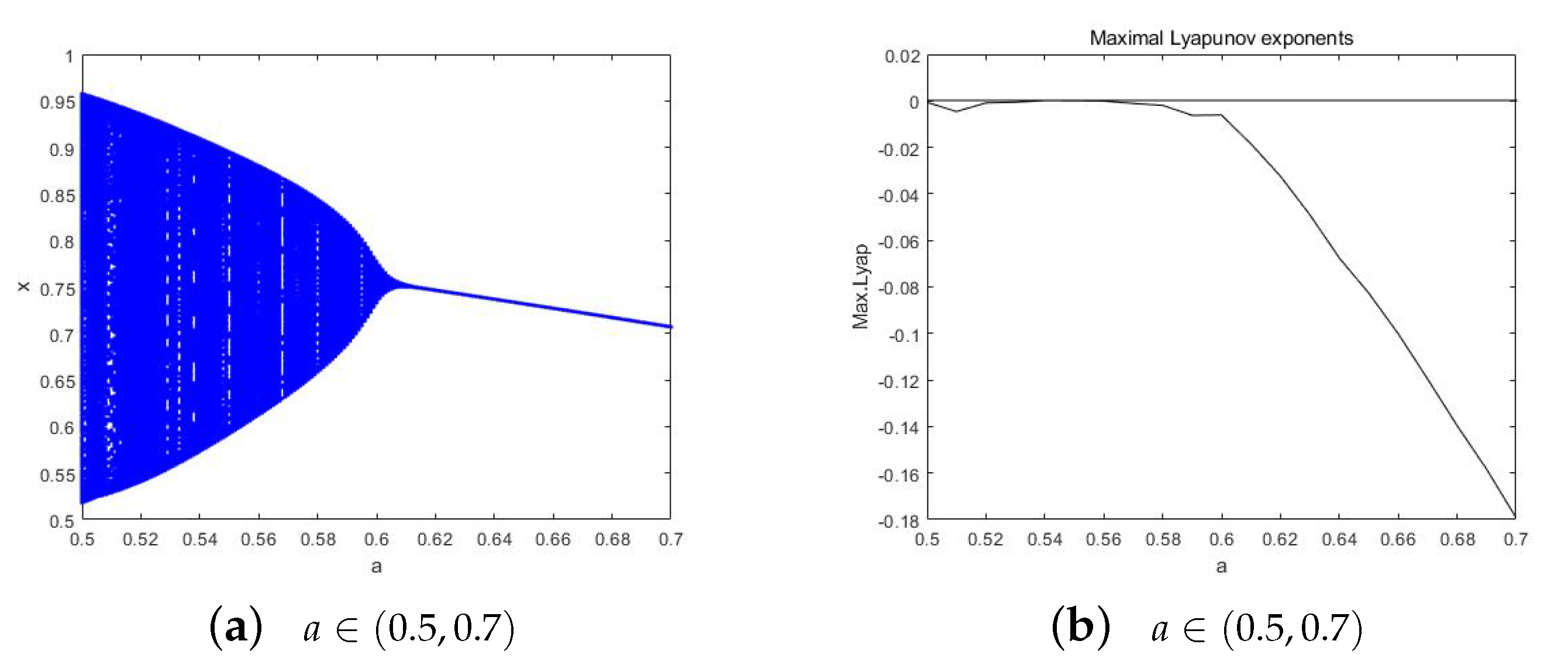
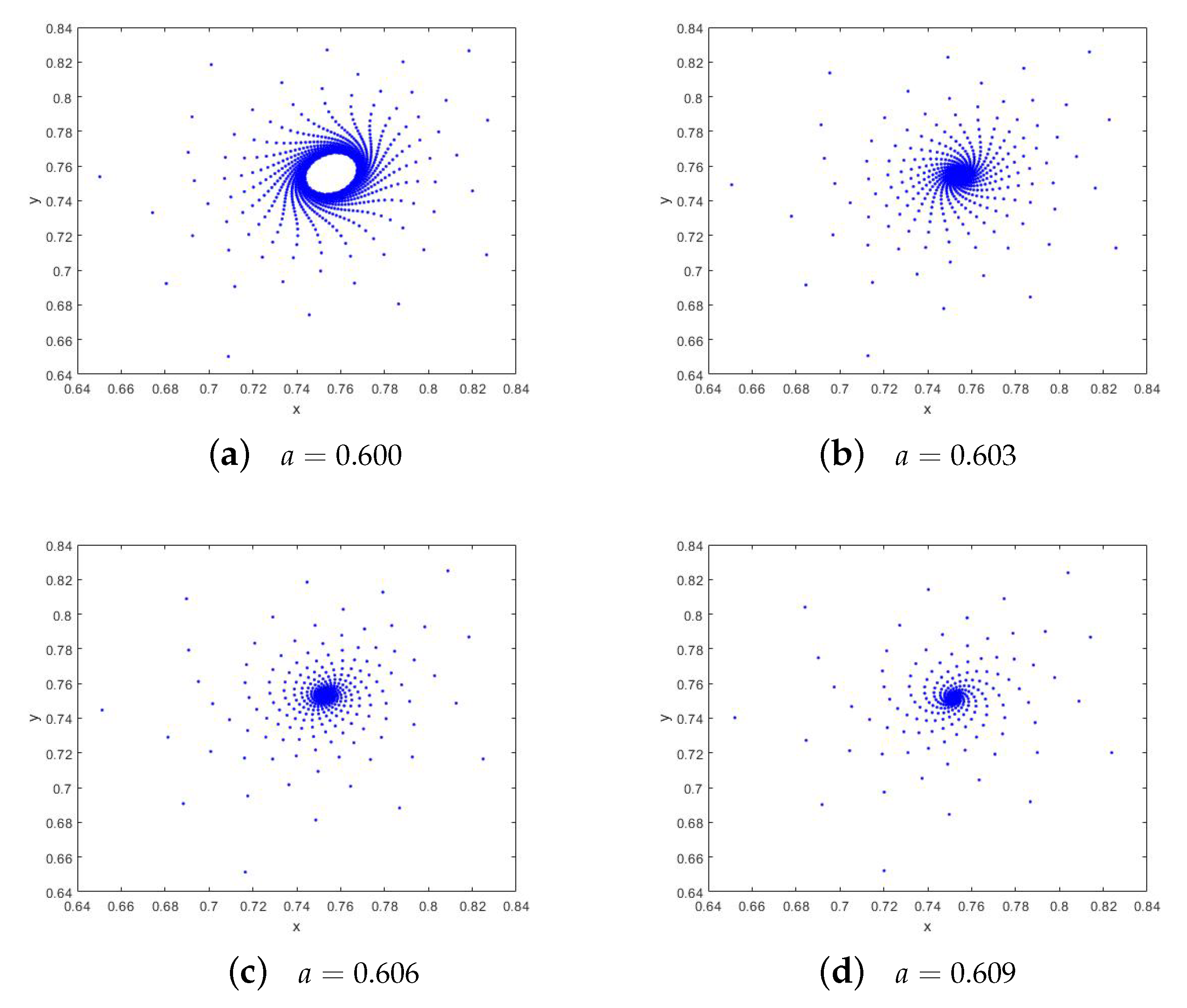
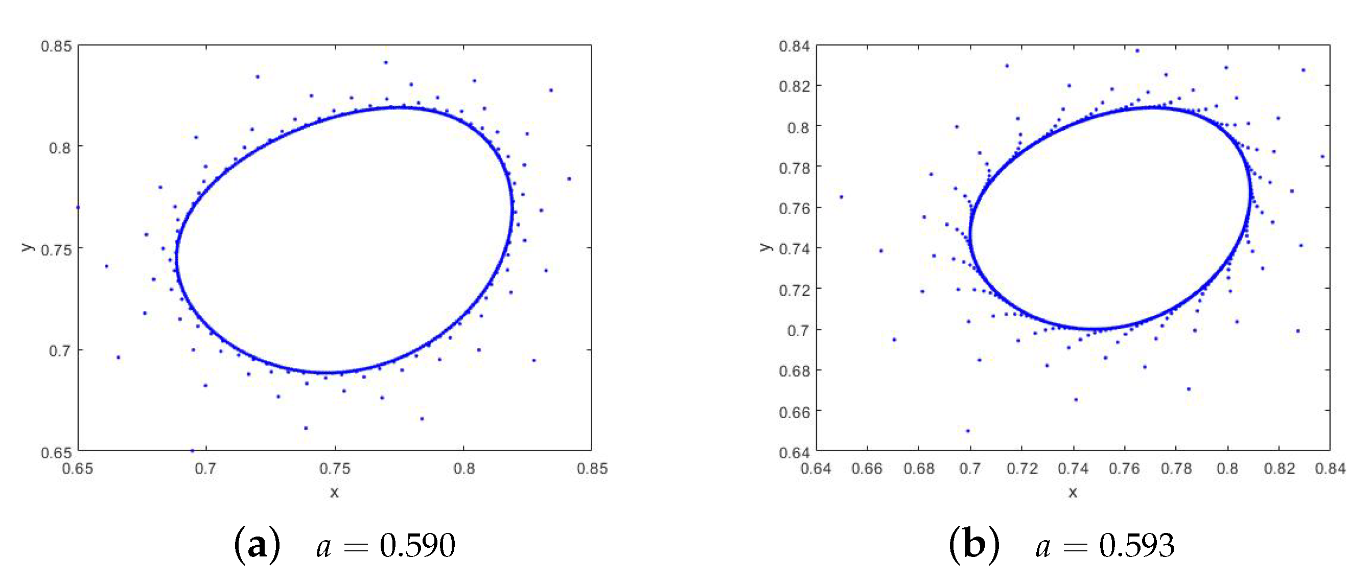
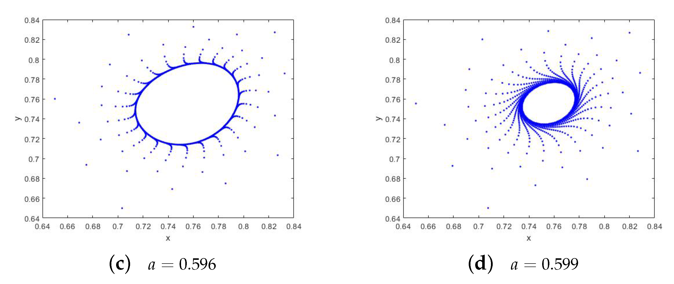
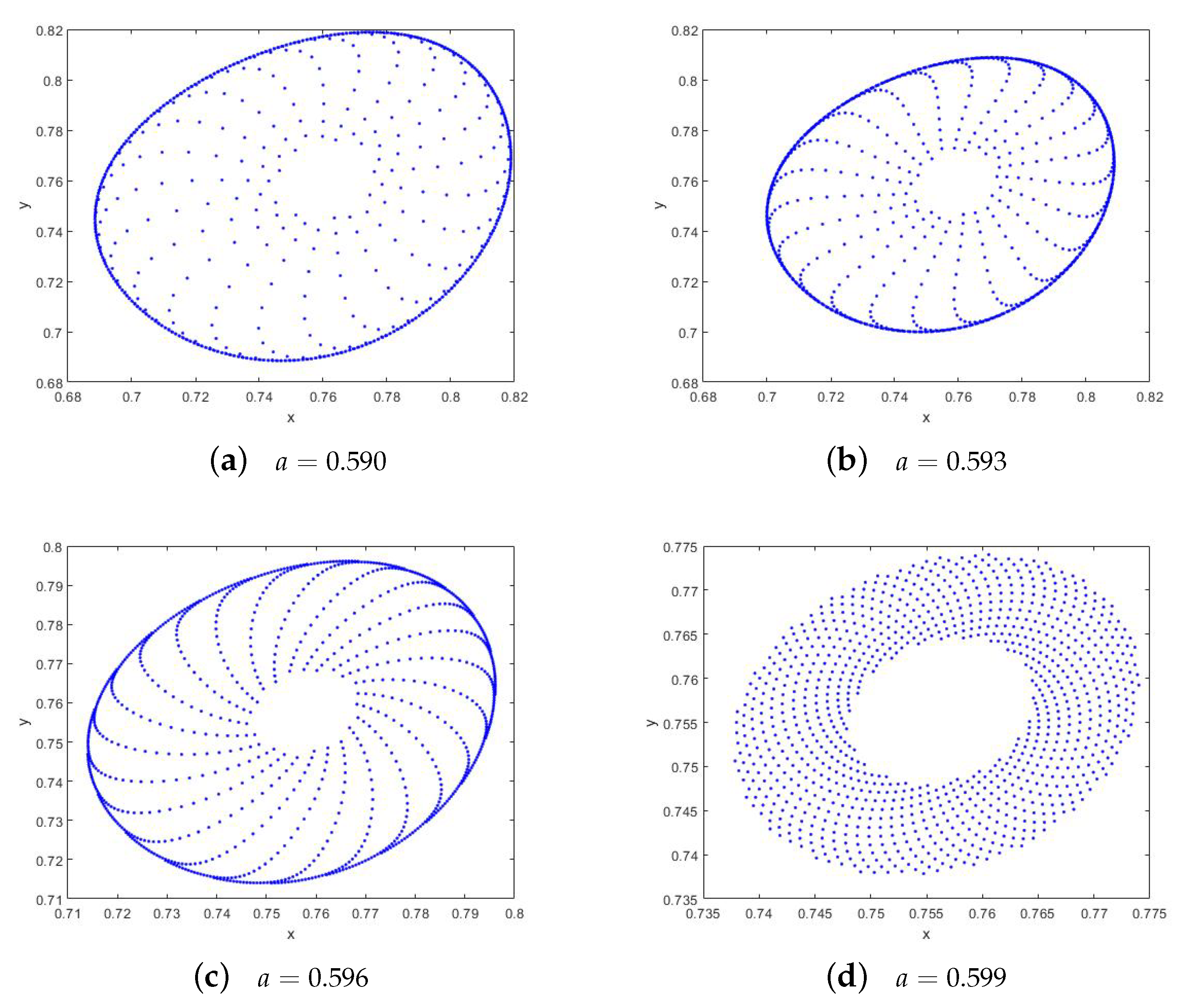
For the fixed point $E_{+},$ choose the parameters $a\in (0.5,0.7),b=1.4$ and the initial values $(x_0,y_0)=(0.05,0.05),(0.75,0.75).$ From Figure 1a we can find that when $a=a_0=0.6$ the system (10) undergoes a Neimark–Sacker bifurcation. In order to bear out it, we take a near $0.6$ and obtain Figure 1, Figure 2, Figure 3 and Figure 4a–d, which illustrate the existence of Neimark–Sacker bifurcation at the fixed point $E_{+}(\sqrt{4/7},\sqrt{4/7})\approx (0.756,0.756).$ Figure 2a–d mean that the fixed point $E_{+}$ is a stable attractor when $a\to 0.6^{+}$. Moreover, Figure 2a,b and Figure 3a show the occurrence of Neimark–Sacker bifurcation when $a\to 0.6^{-}$. Figure 3 and Figure 4a–d illustrate that increasing the value of a leads to a change of stability of the fixed point $E_{+}$ and the occurrence of an invariant closed curve around $E_{+}$, which fits the results in Theorem 4. The spectrum of the maximum Lyapunov exponent with respect to the parameter $a\in (0.5,0.7)$ when $b=1.4$ is presented in Figure 1b.

Remark 1. 

Figure 3a–d show that the bifurcated closed orbit is stable outside whereas Figure 4a–d show that the bifurcated closed orbit is stable inside. Thus, the closed orbit bifurcated from $E_{+}$ is stable. This is in accord with our Theorem 4.

5. Conclusions

In this paper, we apply the semidiscretization method to a delay differential equation considered in [5] and derive a delay difference equation. By using the bifurcation theory, we mainly obtain some results for the Neimark–Sacker bifurcation of the discrete model.

Neimark–Sacker bifurcation is an important mechanic for one system to produce complicated dynamical behaviors. The occurrence of a Neimark–Sacker bifurcation often causes the system to jump from a stable window to chaotic states through periodic and quasi-periodic states and triggers a route to chaos. We find this mechanic in the delay difference equation. Whether or not there are other similar bifurcation problems, such as flip bifurcation, fold bifurcation, etc., in other delay difference equations, and how to find such bifurcations, will be an interesting and important topic and a direction worth future study.