Efficient Solution of Burgers’, Modified Burgers’ and KdV–Burgers’ Equations Using B-Spline Approximation Functions

Abstract

This paper discusses the application of the orthogonal collocation on finite elements (OCFE) method using quadratic and cubic B-spline basis functions on partial differential equations. Collocation is performed at Gaussian points to obtain an optimal solution, hence the name orthogonal collocation. The method is used to solve various cases of Burgers’ equations, including the modified Burgers’ equation. The KdV–Burgers’ equation is considered as a test case for the OCFE method using cubic splines. The results compare favourably with existing results. The stability and convergence of the method are also given consideration. The method is unconditionally stable and second-order accurate in time and space.

1. Introduction

Collocation methods have been preferred to other numerical methods, such as the finite difference and Galerkin methods, because they are simple and easy to implement, the evaluation of integrals is not required, their collocation matrix has a small band width [1] and they yield global approximations. Spline collocation employs a linear combination of piecewise polynomials called spline basis functions to solve differential equations. Using a B-spline representation, the basis functions do not show spurious oscillations as do higher-order polynomial approximations [2]. Improvements on approximations with B-splines have been made through partitioning the required intervals into smaller intervals called finite elements [3]. A unique property of orthogonal collocation on finite elements (OCFE) is that the nodes are roots of orthogonal polynomials [4]. OCFE often yields optimal approximate solutions; hence, the application of spline collocation on each element taking Gaussian points as nodes is an example of OCFE. This method has been used to solve various problems in the literature, e.g., Burgers’ equation, the KdV equation and so on.

Burgers’ equation is a popular nonlinear time-dependent partial differential equation which describes different physical phenomena. It is the simplified form of the famous Navier–Stokes equation in fluid dynamics [1]. It is an important mathematical model that has applications in fluid dynamics, the theory of shock waves, elasticity, heat conduction and traffic flow [1]. It has known exact solutions in the literature. Many numerical methods have been applied to solve Burgers’ equation. The list includes the homotopy perturbation method [5], the homotopy analysis method [6], finite difference [7], the Adomian decomposition method [8,9], spline collocation [1] and the variational iteration method [10], just to mention a few.

The authors in [11] examined optimal error bounds for cubic spline interpolation. In [12], a cubic B-spline collocation method to solve convection–diffusion equations with different Dirichlet boundary conditions was discussed. The authors concluded that their method was unconditionally stable and compared favourably with earlier results in the literature. A detailed analysis and application of orthogonal spline collocation (OSC) to partial differential equations and initial-boundary value problems (IBVPs) was presented in [13]. A numerical scheme to solve Burgers’ equation using quintic Hermite spline collocation on finite elements was proposed in [1]. Cubic B-spline collocation on finite elements was used to obtain the solution of Burgers’ equation in [14]. A modified cubic spline quadrature method was used to solve Burgers’ equation in [15]. The modification produced a diagonally dominant coefficient matrix, which is also tridiagonal and easily solved using the Thomas algorithm. Reference [16] discussed the convergence analysis of orthogonal spline collocation for Burgers’ equation using the extrapolated Crank–Nicholson method for discretization in time. It was found that the error at every time step is of order two in time and $s+1$ in space for splines whose degree is $s\ge 3$. In [17], a Dirichlet biharmonic problem was approximated via the quadratic spline collocation method. An extensive review of the properties and application of B-splines to fluid dynamics was discussed in [2]. Similarly, the author of [4] reviewed the development of the method of weighted residuals and showed the equivalence of orthogonal collocation, the pseudospectral method and the differential quadrature method. Paper [18] discussed the approximate solutions of ordinary differential equations of any order using collocation at Gaussian points together with the global error associated with the solution. It was shown in [19] that the quadratic spline collocation method performed better than cubic splines in terms of the accuracy of the numerical solution of two-point boundary value problems when collocating at equally spaced points. Based on the quadratic spline basis, [20] solved the regularized long-wave equation. In addition, [3] applied collocation based on quintic Hermite basis functions on finite elements at Gaussian points to solve third-order ordinary differential equations and time-dependent partial differential equations.

Burgers’ equation has received much attention to the extent that the generalized form of Burgers’ equation is now being considered. The modified Burgers’ equation has applications in ion reflection at quasi-perpendicular shocks, transport of pollutants and nonlinear waves in a medium with low-frequency absorption [21]. It has been studied by many researchers applying different methods to obtain its numerical solutions. Burgers’ equation and the modified Burgers’ equation were examined in [22] using the sextic B-spline collocation approach. The authors in [21] provided error bounds for septic Hermite splines with orthogonal collocation. They applied quasilinearization and the Crank–Nicolson method for time integration to achieve an unconditionally stable scheme. A second-order exponential time differencing scheme was used by [23] to solve Burgers’ equation and its modified form. A discussion on quintic spline collocation for the modified Burgers’ equation was carried out in [24], while [25] examined the modified Burgers’ equation using the quintic B-spline collocation method.

Of great interest is the Korteweg–de Vries–Burgers’ (KdVB) equation, which consists of both KdV and Burgers’ equations. It has applications in modelling shallow water waves and nonlinear systems due to the presence of dispersion and damping terms [26]. The He’s variational iteration method was used in [27] to obtain the solution of the KdVB equation. Among others who have worked on the KdVB equation are [26,28], who applied quintic B-spline collocation and the Adomian decomposition (ADM) method, respectively. The work by the authors of [29] compared the solutions of KdVB using the finite difference and Adomian decomposition methods. In [30], the exact travelling wave solution of the KdVB equation was studied, and that of a compound KdV–Burgers’ equation was presented in [31] using the homogeneous balanced method. It was suggested in [31] that some particular variations of the KdV–Burgers’ equation can be solved using the homogeneous balance method. Exact solutions to the KdV–Burgers’ equation were constructed in [32] using two different methods, one of which is based on the series approach and is typically an extension of Hirota’s method. In [33], both KdV and KdV–Burgers’ equations were solved using the modified tanh–coth method, and new multiple travelling wave solutions were obtained. The work in paper [34] showed that the new multiple solutions obtained in [33] were actually not new but transformed known solutions of the KdV and KdV–Burgers’ equations. A new approach to solve the extended KdV equation was discussed in [35] via the Galerkin finite element method with quintic B-spline functions as weight functions.

In this paper, we propose the OCFE method using quadratic and cubic B-splines and quasilinearization. Subsequently, the OCFE method is applied to solve Burgers’ equation and the modified Burgers’ and KdV–Burgers’ equations. The main advantages of the proposed method as compared to other methods mentioned above are as follows: (1) there is no need to solve large nonlinear systems of equations; (2) the boundary conditions are enforced strongly, so there is no need to introduce fictional points (knots) or additional equations; (3) the solution values are readily available at the grid points; (4) the OCFE method yields better convergence rates than the classical B-spline collocation method; and (5) the OCFE method can be adapted to dynamically track the profile of rapidly varying transients using an adaptive grid (placing more elements) where the solution is changing rapidly. However, we do not pursue the latter here.

The arrangement of the remaining sections of this paper are as follows: we describe quadratic spline collocation in Section 2 and Section 3; application of quadratic B-spline collocation to Burgers’ equation is discussed in Section 4; a linearization approach to fix errors arising from temporal variations and nonlinearity of Burgers’ equation is presented in Section 5; stability of the method is considered in Section 6; convergence of the method is discussed in Section 7; and numerical examples and simulations for Burgers’ equation are given in Section 8. In Section 9, the OCFE method is applied to the modified Burgers’ equation, and the numerical results are reported in Section 10. Section 11, Section 12 and Section 13 are dedicated to using the OCFE method, employing cubic B-splines to solve the KdV–Burgers’ equation. In Section 14, we treat a special case of Kdv–Burgers’ equation that has no exact solution. Finally, Section 15 concludes the paper.

2. B-Spline Basis

Consider a non-decreasing sequence of knots,

$$z_1\le z_2\le \cdots \le z_k\le z_{k+1}\cdots \le z_{N+1}$$

Each B-spline curve has the form $p\left(z\right)={\displaystyle \sum _{i=1}^{N+1}}{\beta }_i{B}_{i,k}\left(z\right)$ where ${\beta }_i$ is the constant and $B_{i,k}\left(z\right)$ is a normalized basis function. The order of the basis function is k, and the degree of the polynomial is $k-1$. Some properties of B-spline curves are listed below

• $p\left(z\right)$ is a polynomial of degree $k-1$ on $z_i\le z<z_{i+1}$.
• $p\left(z\right)\in C^{k-2}(z_1,z_{N+1})$.
• The sum of the basis functions are identical unity or ${\displaystyle \sum _{i=1}^k}{B}_{i,k}\left(z\right)=1$.
• Each $B_{i,k}\left(z\right)>0$ on $(z_i,z_{i+k})$.
• Each basis function has one maximum value, except in the case of $k=1$.

In order to calculate the basis functions, we need the knot vectors, which are usually written as $[z_i,z_{i+1},\cdots ,z_{i+p}]$ where $p+1$ denotes the number of knots. There are three types of knot vectors: (1) uniform knots, which are evenly spaced; (2) non-uniform knots, which are irregularly spaced; and (3) open uniform knots. The multiplicities of the knots at the ends are equal to the order of the basis, and the knots are equally spaced. We shall consider only the third type and only two distinct knots. Once the knots have been chosen, the basis is calculated using the Cox–de Boor recursion formula [18],

$$B_{i,1}\left(z\right)=\left\{\begin{array}{cc}1,\hfill & [z_i,z_{i+1}),\hfill \\ 0,\hfill & \mathrm{otherwise},\hfill \end{array}\right.$$

(1)

$$B_{i,k}\left(z\right)=\frac{z-z_i}{z_{i+k-1}-z_i}{B}_{i,k-1}\left(z\right)-\frac{z-z_{i+k}}{z_{i+k}-z_{i+1}}{B}_{i+1,k-1}\left(z\right).$$

(2)

Here, for the recursion to work, we adopt the notation $0/0=0.$

3. Quadratic Basis and Orthogonal Collocation on Finite Elements

In this case, $k=3$, and we use the knots $[z_1,z_2,z_3,z_4,z_5,z_6]=[0,0,0,1,1,1]$. The multiplicity at the end points 0 and 1 is three, and there are two distinct knots.

From the recursion Formula (2), it is evident that in order to determine $B_{i,3}\left(z\right),i=1,2,3$, we require $B_{i,2}\left(z\right),i=1,2,3,4$ as well as $B_{i,1}\left(z\right),i=1,2,3,4,5.$ From the definition of $B_{i,1}\left(z\right)$, it follows that $B_{1,1}\left(z\right)=B_{2,1}\left(z\right)=B_{4,1}\left(z\right)=B_{5,1}\left(z\right)=0$ and $B_{3,1}\left(z\right)=1$ in $[z_3,z_4]=[0,1]$. One can also confirm from the recurrence relation that $B_{1,2}\left(z\right)=B_{4,2}\left(z\right)=0,B_{2,2}\left(z\right)=1-z$ and $B_{3,2}\left(z\right)=z^2$. Hence, the recurrence relation gives

$$B_{1,3}\left(z\right)={(1-z)}^2,B_{2,3}=2z(1-z)\mathrm{and}{B}_{3,3}\left(z\right)=z^2.$$

We observed that if we expand ${[z+(1-z)]}^{k-1}$ using the binomial theorem, then we can recover the quadratic basis $B_{i,k},i=1,2,3$, where k is the order of the spline. Let $B_1\left(z\right)={(1-z)}^2$, $B_2\left(z\right)=2z(1-z)$, $B_3\left(z\right)=z^2$, where we have dropped the subscript.

For ease of explanation of the OCFE method, we solve a second-order ODE given via

$$a_2\left(x\right)y^{″}\left(x\right)+a_1\left(x\right)y^{\prime }\left(x\right)+a_0\left(x\right)y\left(x\right)=f\left(x\right),x\in (a,b),$$

(3)

with the boundary conditions

$$y\left(a\right)=\theta ,y\left(b\right)=\Theta .$$

(4)

Suppose we partition the interval $[a,b]$ into N elements with nodes given via $x_i=a+(i-1)h$, $i=1,2,\dots ,N+1$, where $h=\frac{b-a}{N}$ is the uniform step size. The transformation $z=\frac{x-x_i}{x_{i+1}-x_i}=\frac{x-x_i}{h}$ maps the $i_{th}$ interval $\left[x_i{x}_{i+1}\right]$ to $[0,1]$. The collocation solution in interval i and interval $(i+1)$ is respectively assumed to be $Y^i\left(x\right)={\displaystyle \sum _{k=1}^3}{b}_k^i{B}_k\left(x\right)$ and $Y^{i+1}\left(x\right)={\displaystyle \sum _{k=1}^3}{b}_k^{i+1}{B}_k\left(x\right).$ To enforce continuity at internal boundaries, we write

$$Y^{i+1}\left(x_{i+1}\right)=Y^i\left(x_{i+1}\right),{\left.\frac{d{Y}^{i+1}}{dx}\right|}_{x_{i+1}}={\left.\frac{d{Y}^i}{dx}\right|}_{x_{i+1}}.$$

(5)

$$\Rightarrow Y^{i+1}\left(0\right)=Y^i\left(1\right),{\left.\frac{d{Y}^{i+1}}{dz}\right|}_{z=0}={\left.\frac{d{Y}^i}{dz}\right|}_{z=1},i=1,2,\dots ,N-1.$$

(6)

$$\Rightarrow b_1^{i+1}=b_3^i,b_2^{i+1}=2b_3^i-b_2^i.$$

(7)

Then, for each element i, we may write

$$Y\left(z\right)={\displaystyle \sum _{k=1}^3}{b}_{k+2(i-1)}{B}_k\left(z\right),i=1,2,\dots ,N.,$$

(8)

Discretization of (3) into finite elements, and substitution of (8) in (3) together with (4), yields

$${\displaystyle \sum _{k=1}^3}\left[\frac{a_2\left(z\right)}{h^2}{B}_k^{″}\left(z\right)+\frac{a_1\left(z\right)}{h}{B}_k^{\prime }\left(z\right)+a_0\left(z\right)B_k\left(z\right)\right]b_{k+2(i-1)}=f(x_i+hz),i=1,2,\dots ,N$$

(9)

and

$$y\left(0\right)=b_1=\theta ,y\left(1\right)=b_{2N+1}=\Theta .$$

(10)

Equation (9) contains $2N+1$ unknowns; hence, we require $2N+1$ conditions. In order to achieve this, we use one collocation point per element, namely $z=0.5$ in (9), which, together with the two boundary conditions and $N-1$ continuity equations from (7), results in a closed linear system of the form $A\mathbf{b}=\mathbf{g}$. The coefficient matrix A has the form

$$A=\left[\begin{array}{ccccccccccccc}{M}_1& M_2& M_3& 0& 0& 0& 0& 0& 0& \cdots & 0& 0& 0\\ 0& 0& M_1& M_2& M_3& 0& 0& 0& 0& \cdots & 0& 0& 0\\ 0& 0& 0& 0& M_1& M_2& M_3& 0& 0& \cdots & 0& 0& 0\\ 0& 0& 0& 0& 0& 0& M_1& M_2& M_3& \cdots & 0& 0& 0\\ ⋮& ⋮& ⋮& ⋮& ⋮& ⋮& ⋮& ⋮& ⋮& \cdots & ⋮& ⋮& ⋮\\ 0& 0& 0& 0& 0& 0& 0& 0& 0& \cdots & M_1& M_2& M_3\\ 0& -1& 2& -1& 0& 0& 0& 0& 0& \cdots & 0& 0& 0\\ 0& 0& 0& -1& 2& -1& 0& 0& 0& \cdots & 0& 0& 0\\ 0& 0& 0& 0& 0& -1& 2& -1& 0& \cdots & 0& 0& 0\\ ⋮& ⋮& ⋮& ⋮& ⋮& ⋮& ⋮& ⋮& ⋮& \cdots & ⋮& ⋮& ⋮\\ 0& 0& 0& 0& 0& 0& 0& 0& 0& \cdots & 2& -1& 0\\ 1& 0& 0& 0& 0& 0& 0& 0& 0& \cdots & 0& 0& 0\\ 0& 0& 0& 0& 0& 0& 0& 0& 0& \cdots & 0& 0& 1\end{array}\right],$$

(11)

$$M_j=\frac{a_2\left(0.5\right)}{h^2}{B}_j^{″}\left(0.5\right)+\frac{a_1\left(0.5\right)}{h}{B}_j^{\prime }\left(0.5\right)+a_0\left(0.5\right)B_j\left(0.5\right),j=1,2,3$$

(12)

and vector of unknowns $\mathbf{b}={[b_1,b_2,b_3,\cdots ,b_{2N+1}]}^T$, where T represents the transpose and

$$g_i=\left\{\begin{array}{cc}f(x_i+0.5h)\hfill & i=1,\dots ,N,\hfill \\ 0\hfill & i=N+1,\dots ,2N-1,\hfill \\ \theta \hfill & i=2N,\hfill \\ \Theta \hfill & i=2N+1.\hfill \end{array}\right.$$

(13)

Numerical Example

As a test case of (3) and (4), we consider the following BVP [19]:

$$y^{″}-100y=0,y\left(0\right)=y\left(1\right)=1.$$

The exact solution is given via

$$y=cosh(10x-5)/cosh\left(5\right).$$

Table 1 belowshows the order of convergence using the OCFE method and the classical collocation method using quadratic splines studied in [19]. As expected, the OCFE method converges faster than the classical quadratic spline collocation method.

Table 1. Orderof Convergence.

h	Khalifa [19]	OCFE
$\frac{1}{20}$	1.76	2.12
$\frac{1}{40}$	1.93	2.03
$\frac{1}{80}$	1.96	2.00

Here, the order of convergence is given via ${log}_2\frac{\left|\right|{\mathbf{e}}_i{\left|\right|}_{\infty }^h}{\left|\right|{\mathbf{e}}_i{\left|\right|}_{\infty }^{h/2}}$ where ${\mathbf{e}}_i=\mathbf{y}\left({\mathbf{x}}_i\right)-\mathbf{Y}\left({\mathbf{x}}_i\right)$ is the error vector at the nodes.

We study the OCFE method in greater detail in the following sections. We begin with the application of the OCFE method to Burgers’ equation.

4. Application to Burgers’ Equation

Consider Burgers’ equation

$$u_t=\nu u_{xx}-u{u}_x,a<x<b,t\ge t_0,$$

(14)

with the boundary conditions

$$u(a,t)=\theta ,u(b,t)=\Theta$$

(15)

and initial condition

$$u_0\left(x\right)=u(x,t_0).$$

(16)

For a partial differential equation (PDE) in space and time, we write the trial solution as

$$u(z,t)={\displaystyle \sum _{k=1}^3}{b}_{k+2(i-1)}\left(t\right)B_k\left(z\right).$$

(17)

Discretization of (14) into finite elements and substitution of (17) in (14) yields

$$\begin{array}{cc}\hfill & {\displaystyle \sum _{k=1}^3}{b}_{k+2(i-1)}^{\prime }\left(t\right)B_k\left(z\right)=\frac{\nu }{h^2}{\displaystyle \sum _{k=1}^3}{b}_{k+2(i-1)}\left(t\right)B_k^{″}\left(z\right)\hfill \\ & -\frac{1}{h}\left({\displaystyle \sum _{k=1}^3}{b}_{k+2(i-1)}\left(t\right)B_k\left(z\right)\right)\left({\displaystyle \sum _{k=1}^3}{b}_{k+2(i-1)}\left(t\right)B_k^{\prime }\left(z\right)\right),i=1,2,\dots ,N.\hfill \end{array}$$

(18)

The boundary conditions (15) (for simplicity, choosing $a=0,b=1$) yield

$$b_1\left(t\right)=\theta ,b_{2N+1}\left(t\right)=\Theta .$$

(19)

Equations (18) and (19) give a system of differential-algebraic equations (DAEs) which has to be solved in time. Unfortunately, for large N, solving this system could prove to be computationally challenging. A common alternative used in the literature, which avoids dealing with DAEs, is to use the Crank–Nicolson method with quasi-linearization to accomplish time integration. Furthermore, the stability and convergence of the method is easily established. In the next section, we apply the quasilinearization method to Burgers’ equation.

5. Application of Quazilinearization to Burgers’ Equation

Applying linearization and the trapezoid rule to Burgers’ equation yields

$$\begin{array}{cc}\hfill \left[1+\frac{\Delta t}{2}{u}_x(x,t_j)\right]u(x,t_{j+1})& -\frac{\nu \Delta t}{2}{u}_{xx}(x,t_{j+1})+\frac{\Delta t}{2}u(x,t_j)u_x(x,t_{j+1})\hfill \\ & =u(x,t_j)+\frac{\nu \Delta t}{2}{u}_{xx}(x,t_j).\hfill \end{array}$$

(20)

Since

$$u(x,t_j)={\displaystyle \sum _{k=1}^3}{b}_{k+2(i-1)}\left(t_j\right)B_k\left(x\right),$$

(21)

using the transformation $z=\frac{x-x_i}{h}$ in (20), we have

$$\begin{array}{cc}\hfill & {\displaystyle \sum _{k=1}^3}\left(\left[1+\frac{\Delta t}{2h}{\displaystyle \sum _{k=1}^3}{b}_{k+2(i-1)}\left(t_j\right)B_k^{\prime }\left(z\right)\right]B_k\left(z\right)-\frac{\Delta t}{2h^2}\nu B_k^{″}\left(z\right)\right.\hfill \\ & \left.+\frac{\Delta t}{2h}\left[{\displaystyle \sum _{k=1}^3}{b}_{k+2(i-1)}\left(t_j\right)B_k\left(z\right)\right]B_k^{\prime }\left(z\right)\right)b_{k+2(i-1)}\left(t_{j+1}\right)\hfill \\ & ={\displaystyle \sum _{k=1}^3}\left[B_k\left(z\right)+\frac{\Delta t}{2h^2}\nu B_k^{″}\left(z\right)\right]b_{k+2(i-1)}\left(t_j\right),i=1,2,\dots ,N.\hfill \end{array}$$

(22)

Substituting one collocation point per interval for z in Equation (22) and using the boundary conditions will give a system of equations of the form $Q\mathbf{b}\left(t_{j+1}\right)=P\mathbf{b}\left(t_j\right).$

6. Stability of the Quadratic B-Spline Collocation Method

The von Neumann analysis technique is used to determine the stability of a numerical method for linear initial value problems and linearized nonlinear boundary value problems.

Let $K=max\left\{u\right\}$ be a local constant representing u in the nonlinear term of Equation (14), and use the Crank–Nicolson method for discretization. We have

$$u^{n+1}+\frac{\Delta tK}{2}{u}_x^{n+1}-\frac{\Delta t}{2}{u}_{xx}^{n+1}=u^n-\frac{\Delta tK}{2}{u}_x^n+\frac{\Delta t}{2}{u}_{xx}^n,$$

(23)

where $\Delta t$ is the time step. Suppose $\alpha =\frac{\Delta tK}{h}$ and $\beta =\frac{\Delta t\nu }{h^2}$. We have

$$u^{n+1}+\frac{\alpha }{2}{u}_z^{n+1}-\frac{\beta }{2}{u}_{zz}^{n+1}=u^n-\frac{\alpha }{2}{u}_z^n+\frac{\beta }{2}{u}_{zz}^n.$$

(24)

Since

$$u^n\left(z\right)={\displaystyle \sum _{l=1}^3}{b}_{l+2(m-1)}^n{B}_l\left(z\right),$$

(25)

Equation (24) can be written as

$${\displaystyle \sum _{l=1}^3}{b}_{l+2(m-1)}^{n+1}\left[B_l\left(z\right)+\frac{\alpha }{2}{B}_l^{\prime }\left(z\right)-\frac{\beta }{2}{B}_l^{″}\left(z\right)\right]={\displaystyle \sum _{l=1}^3}{b}_{l+2(m-1)}^n\left[B_l\left(z\right)-\frac{\alpha }{2}{B}_l^{\prime }\left(z\right)+\frac{\beta }{2}{B}_l^{″}\left(z\right)\right].$$

(26)

Then, at the collocation point $z=\frac{1}{2}$,

$$b_{2m-1}^{n+1}{\sigma }_1+b_{2m}^{n+1}{\sigma }_2+b_{2m+1}^{n+1}{\sigma }_3=b_{2m-1}^n{\rho }_1+b_{2m}^n{\rho }_2+b_{2m+1}^n{\rho }_3,$$

(27)

where

$$\begin{array}{ll}{\rho }_1=\frac{1}{4}-\frac{\alpha }{2}+\beta ,& {\sigma }_1=\frac{1}{4}+\frac{\alpha }{2}-\beta ,\\ {\rho }_2=\frac{1}{2}-2\beta ,& {\sigma }_2=\frac{1}{2}+2\beta ,\\ {\rho }_3=\frac{1}{4}+\frac{\alpha }{2}+\beta ,& {\sigma }_3=\frac{1}{4}-\frac{\alpha }{2}-\beta .\end{array}$$

Let $b_l^n={\lambda }^n{e}^{ilhk}$, k= mode and $i=\sqrt{-1}$, then (27) gives

$$\begin{array}{cc}\hfill & {\lambda }^{n+1}\left[e^{i(2m-1)hk}{\sigma }_1+e^{i2mhk}{\sigma }_2+e^{i(2m+1)hk}{\sigma }_3\right]={\lambda }^n\left[e^{i(2m-1)hk}{\rho }_1+e^{i2mhk}{\rho }_2+e^{i(2m+1)hk}{\rho }_3\right],\hfill \end{array}$$

(28)

$$\Rightarrow \lambda =\frac{E_1+i{F}_1}{E_2+i{F}_2},$$

(29)

where $E_1=2{\rho }_{1}coshk+{\rho }_2+\alpha cos\left(hk\right)$, $E_2=2{\sigma }_{1}coshk+{\sigma }_2-\alpha cos\left(hk\right)$, $F_1=\alpha sin\left(hk\right)$, and $F_2=-\alpha sin\left(hk\right).$ It is easy to show that $\left|\lambda \right|\le 1$. This shows that orthogonal quadratic spline collocation on finite elements using Gauss points for Burgers’ equation is unconditionally stable.

7. Convergence of the Method

We assume that the exact solution of Equation (14) is $\overline{u}(x,t)\in C^4[a,b]\times C^2[t_0,t_f]$, where $t_0$ and $t_f$ are initial and final times, respectively. From the trapezoid rule, the local error is given using $\frac{\Delta t^3}{12}{u}_{tt}(x,{\xi }_j),{\xi }_j\in [t_j,t_{j+1}].$

Let $u_L(x,t_{j+1})$ be the exact solution of (20), and assume that $u_L(x,t_{j+1})\in C^4[a,b].$ At time $t_{j+1}$, the global error is $t_{j+1}{K}^{\prime }\Delta t^2$ for constant $K^{\prime }$. Hence

$$\left|\right|\overline{u}(x,t_{j+1})-u_L(x,t_{j+1}){\left|\right|}_{\infty }\le K\Delta t^2$$

(30)

for some constants $K.$

We let $u(x,t_j)=u^j\left(x\right)$, then Equation (20) becomes

$$u_{xx}^{j+1}\left(x\right)-a_1\left(x\right)u_x^{j+1}\left(x\right)-a_0\left(x\right)u^{j+1}\left(x\right)=f\left(x\right).$$

(31)

We assume that $a_0\left(x\right),a_1\left(x\right)\in C^2[a,b].$ Let $u_c(x,t)\in P_3\cap C^1[a,b]$ be the collocation solution to (31), where $P_3$ denotes polynomials of degree < 3. From de Boor [18],

$$|D^{\left(i\right)}(u_L^{j+1}-u_c^{j+1})\left(x_p\right)|\le C_1{h}^2,$$

(32)

and

$$\left|\right|D^{\left(i\right)}(u_L^{j+1}-u_c^{j+1})\left(x_p\right){\left|\right|}_{\infty }\le C_1{h}^{1+min(1,2-i)},i=0,1,2.$$

(33)

Inequalities (30) and (32) imply

$$\left|\right|\overline{u}(x,t_{j+1})-u_c(x,t_{j+1}){\left|\right|}_{\infty }\le K\Delta t^2+C_1{h}^2.$$

(34)

We now show that the collocation matrix system of Equation (31) has a unique solution for any number of finite elements N. The resulting coefficient matrix is a square matrix of the order $2N+1$. It may be shown using elementary row and column operations that the coefficient matrix is equivalent to a block upper triangular matrix. Hence the determinant ${\Delta }_N$ can be deduced to be given via (see Appendix A).

$${\Delta }_N=\frac{-M_2}{2^N\sqrt{{\alpha }^2-4M_1{M}_3}}\left[{\left(\alpha +\sqrt{{\alpha }^2-4M_1{M}_3}\right)}^N-{\left(\alpha -\sqrt{{\alpha }^2-4M_1{M}_3}\right)}^N\right],$$

(35)

where $\alpha =2M_2+M_1+M_3.$

The matrix is non-singular if $M_2\ne 0$ and ${\alpha }^2\ne 4M_1{M}_3$. In this case, a unique solution to the system of equations exists. Hence, the method converges to the solution.

8. Numerical Examples and Simulations for Burgers’ Equation

In this section, we consider various examples and present various numerical simulations to demonstrate the efficiency of the OCFE method.

1.

We compare the results of our method with the work of Raslan [36] on Burgers’ Equation (14). The exact solution to (14) is

$$u(x,t)=\frac{x}{t\left(1+\sqrt{\frac{t}{\tau }}{e}^{\frac{x^2}{4\nu t}}\right)},$$

(36)

where $\tau =exp\left(\frac{1}{8\nu }\right)$, and the initial condition is

$$u_0\left(x\right)=u(x,1).$$

(37)

The boundary conditions are $u(0,t)=0$ and $u(1,t)=0$. Results of our method are presented in Table 2, Table 3 and Table 4 when the number of partitions of the space interval [0, 1] is $N=50$, the number of time steps is $NT=50$ and the final time is $Tf=2$.

Table 2. Error norms at $N=NT=50,Tf=2.$

		${\mathit{L}}_{\mathit{\infty }}$			${\mathit{L}}_2$
t	Present	Raslan [36]	CN	Present	Raslan [36]	CN
1.2	0.002389	0.009445	0.002455	0.003594	0.014613	0.003630
1.4	0.002140	0.009192	0.002201	0.003779	0.019857	0.003762
1.6	0.001868	0.008531	0.001905	0.003589	0.024209	0.003546
1.8	0.001653	0.010477	0.001667	0.003310	0.027808	0.003258
2	0.001431	0.012058	0.001426	0.003025	0.030687	0.002972

Table 3. Invariant at $N=NT=50,Tf=2.$

t	Present	Raslan [36]	CN
1	0.124967	0.124817	0.124967
1.2	0.124059	0.124317	0.124059
1.4	0.123291	0.123954	0.123291
1.6	0.122626	0.123602	0.122626
1.8	0.122039	0.123264	0.122039
2	0.121513	0.122940	0.000000

Table 4. Comparison of $u(x,2)$ at some points $x.$

x	Present	Exact	Raslan [36]
0.365	0.182978	0.182473	0.185924
0.415	0.206938	0.207419	0.215954
0.465	0.232783	0.232227	0.235308
0.605	0.289358	0.288192	0.293358
0.645	0.274683	0.274869	0.279174
0.695	0.181949	0.180506	0.150321
0.725	0.095053	0.098406	0.096996
0.765	0.028298	0.029633	0.030028
0.805	0.006413	0.006911	0.007348
0.845	0.001254	0.001413	0.001598
0.915	6.11 × 10${}^{-5}$	7.05 × 10${}^{-5}$	0.000140

In Table 2, the present results performed better than those of Raslan [36], since both the $L_{\infty }$ and the $L_2$ norm values are better. It is also clear from the table that the $L_{\infty }$ norm of the present work is better than that of the Crank–Nicolson method (CN) based on [36].

The CN based on [36] performed better than Raslan [36], as shown in the table. Hence, both CN and the present method, quadratic B-spline collocation using Gauss points on finite elements, compare favourably.

In Table 3, the invariants for the present work, Raslan [36] and CN based on [36] are compared and found to agree with one another.

Exact solutions of $u(x,2)$ for some values of x are compared in Table 4. The Table shows that the present method converges to the exact solution faster than that of Raslan [36].

In Figure 1, a 3D plot of the exact solution is overlaid onto that of the approximate solution of Burgers’ equation in example 1. It is evident that the approximate and exact solutions match perfectly on the computational domain. Furthermore, in Figure 2, the convergence of the different methods and the CPU times for Raslan [36], the Crank–Nicolson method based on Raslan, and quadratic spline collocation on Gauss points for computation of this example are shown. It is clear that the OCFE method has order-two convergence, and the present method is the fastest of the three methods and nearly five times faster than Raslan [36] and four times faster than CN.

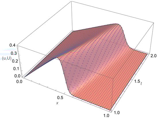
Figure 1. 3D Plot: $N=NT=50.$

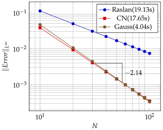
Figure 2. Convergence plot.

2.

A travelling wave solution of Burgers’ Equation (14), which is of the form

$$u(x,t)=\frac{\mu +\alpha +\left(\mu -\alpha \right)e^{\frac{\alpha \xi }{\nu }}}{1+e^{\frac{\alpha \xi }{\nu }}}$$

(38)

with the initial condition

$$u_0\left(x\right)=u(x,0)$$

(39)

and the boundary conditions $u(0,t)=1,u(1,t)=0.2$, where $\xi =x-\mu t-\beta$, $\mu$ and $\alpha$ are constants, is considered. We compare the norms of the errors at various times when the number of partitions of the space interval [0, 1] is $N=50$, the number of time steps is $NT=50$ and the final time is $Tf=2$. Figure 3 shows the profiles at some values of t for all x. The graph of the exact solution is overlaid onto that of the approximate solution in Figure 4. The exact and approximate solutions match perfectly on the computational domain. It is clearly shown in Figure 5 that our method has convergence order two and is three times faster than CN.

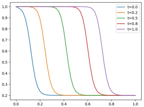Figure 3. Final profiles at different times when $N=NT=50.$

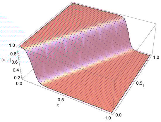Figure 4. 3D plot: $N=NT=50.$

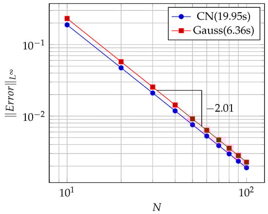Figure 5. Convergence plot.

9. Modified Burgers’ Equation

We apply the OCFE method with a quadratic basis to the modified Burgers’ equation [21,22,23,25]

$$u_t+u^{\delta }{u}_x-\nu u_{xx}=0,\delta \ge 2.$$

(40)

Consider the case of $\delta =2$, $\nu =0.005$ with the initial condition

$$u(x,1)=\frac{x}{1+2e^{\frac{x^2}{4\nu }}}$$

(41)

and boundary conditions

$$u(0,t)=0,u(1,t)=0.$$

(42)

The exact solution is

$$u(x,t)=\frac{x}{t\left(1+2\sqrt{t}{e}^{\frac{x^2}{4\nu t}}\right)}.$$

(43)

Substituting (17) into (40), we get the nonlinear system of equations

$$\begin{array}{cc}\hfill {\displaystyle \sum _{k=1}^3}{b}_{k+2(i-1)}^{\prime }\left(t\right)B_k\left(x\right)& =\frac{\nu }{h^2}{\displaystyle \sum _{k=1}^3}{b}_{k+2(i-1)}\left(t\right)B_k^{″}\left(x\right)\hfill \\ & -\frac{1}{h}{\left({\displaystyle \sum _{k=1}^3}{b}_{k+2(i-1)}\left(t\right)B_k\left(x\right)\right)}^{\delta }\left({\displaystyle \sum _{k=1}^3}{b}_{k+2(i-1)}\left(t\right)B_k^{\prime }\left(x\right)\right).\hfill \end{array}$$

(44)

To simplify the work further, we apply the trapezoidal rule in time, linearize the nonlinear term of Equation (40) and substitute (21) in (40):

$$\begin{array}{cc}\hfill & {\displaystyle \sum _{k=0}^3}\left(\left[1+\frac{\Delta t\delta }{2h}{\left({\displaystyle \sum _{k=0}^3}{b}_{k+2(i-1)}\left(t_j\right)B_k\left(z\right)\right)}^{\delta -1}{\displaystyle \sum _{k=0}^3}{b}_{k+2(i-1)}\left(t_j\right)B_k^{\prime }\left(z\right)\right]B_k\left(z\right)\right.\hfill \\ & \left.-\frac{\Delta t}{2h^2}\nu B_k^{″}\left(z\right)+\frac{\Delta t}{2h}{\left[{\displaystyle \sum _{k=0}^3}{b}_{k+2(i-1)}\left(t_j\right)H_k\left(z\right)\right]}^{\delta }{B}_k^{\prime }\left(z\right)\right)b_{k+2(i-1)}\left(t_{j+1}\right)\hfill \\ & ={\displaystyle \sum _{k=0}^3}\left[B_k\left(z\right)+\frac{\Delta t}{2h^2}\nu B_k^{″}\left(z\right)+\frac{\Delta t}{2h}(\delta -1){\left({\displaystyle \sum _{k=0}^3}{b}_{k+2(i-1)}\left(t_j\right)B_k\left(z\right)\right)}^{\delta }{B}_k^{\prime }\left(z\right)\right]b_{k+2(i-1)}\left(t_j\right).\hfill \end{array}$$

(45)

The boundary conditions become

$$\left\{\begin{array}{c}u(0,t)=b_1=0,\hfill \\ u(1,t)=b_{2N+1}=0.\hfill \end{array}\right.$$

(46)

The system comprising (7), (45) and (46) can now be solved to obtain $u(x,t)$. Clearly, the stability and convergence analysis are very similar to the previous case of the classical Burgers’ equation and are not repeated.

10. Numerical Simulations for the Modified Burgers’ Equation

A 3D plot of the numerical solution and error for $N=50$ are given in Figure 6 and Figure 7, respectively. The orthogonal collocation of finite elements based on quadratic B-spline basis functions gives good results when compared with the exact solution of the modified Burgers’ equation as shown in Figure 7.

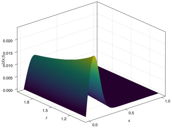
Figure 6. 3D plot of approximated $u(x,t).$

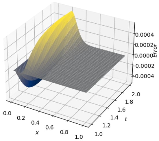
Figure 7. 3D plot of error.

In Figure 8, Figure 9 and Figure 10, time profiles of the solution are shown for various values of $\nu$ and N. It is seen that the OCFE method is capable of tracking the shock propagation of the solution for extremely small values of $\nu$ and moderate values of N.

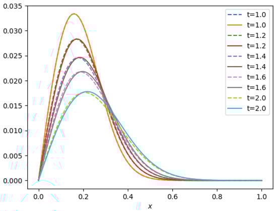
Figure 8. Shock propagation $\nu =0.01$ and $N=100$.

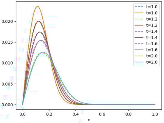
Figure 9. Shock propagation $\nu =0.005$ and $N=100$.

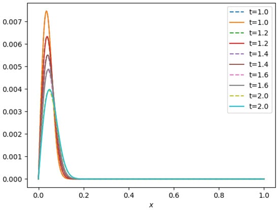
Figure 10. Shock propagation $\nu =0.0005$ and $N=400$.

In the previous sections, we applied quadratic B-splines in conjunction with finite elements (OCFE method) to solve second-order PDEs. It is seen that the OCFE method using quasilinearization is optimal in efficiency for solving Burgers’ and modified Burgers’ equations. In particular, there is no need to impose additional boundary conditions, and the method matches the second-order method used for time integration. Hence, the overall method is second-order in space and time. In the next section, we present the cubic splines OCFE method and demonstrate it’s efficiency for solving third-order PDEs and focus on the KdV–Burgers’ equation. Various numerical experiments are performed to demonstrate the suitability of the cubic B-splines OCFE method.

11. Cubic B-Splines

A spline of order $k=4$, which is a linear combination of third-degree polynomial bases, is called a cubic B-spline. Hence, the required cubic B-spline basis are

$$B_1={(1-z)}^3,B_2=3t{(1-z)}^2,B_3=3z^2(1-z)\mathrm{and}{B}_4=z^3.$$

(47)

Let

$$Y^i\left(x\right)={\displaystyle \sum _{j=1}^4}{b}_j{B}_j\left(x\right)$$

(48)

Consider solving a linear differential equation in one spatial variable x on $(a,b)$. Suppose the interval $[a,b]$ is partitioned into N finite elements. For every element $x\in [x_i,x_{i+1}]$, we transform x into $z\in [0,1]$ via

$$z=\frac{x-x_i}{x_{i+1}-x_i}=\frac{x-x_i}{h}$$

(49)

such that

$$Y^i\left(x\right)=Y^i\left(z\right)={\displaystyle \sum _{j=1}^4}{b}_j{B}_j^i\left(z\right),i=1,2,\dots ,N+1$$

(50)

on the ith element. We now require continuity at the internal boundaries such that

$$\begin{array}{cc}\hfill Y^i\left(x_{i+1}\right)& =Y^{i+1}\left(x_{i+1}\right)\hfill \end{array}$$

(51)

$$\begin{array}{cc}\hfill {\left.\frac{d{Y}^i}{dx}\right|}_{x_{i+1}}& ={\left.\frac{Y^{i+1}}{dx}\right|}_{x_{i+1}}\hfill \end{array}$$

(52)

$$\begin{array}{cc}\hfill {\left.\frac{d^2{Y}^i}{d{x}^2}\right|}_{x_{i+1}}& ={\left.\frac{d^2{Y}^{i+1}}{d{x}^2}\right|}_{x_{i+1}}\hfill \end{array}$$

(53)

Equations (51)–(53) lead to

$$\begin{array}{cc}\hfill g_{4(j-1)}& =g_{4j-3}\hfill \end{array}$$

(54)

$$\begin{array}{cc}\hfill g_{3j-1}& =2g_{3j-2}-g_{3j-3}\hfill \end{array}$$

(55)

$$\begin{array}{cc}\hfill g_{3j}& =g_{3j-4}-4g_{3j-3}+4g_{3j-2}\hfill \end{array}$$

(56)

where $j=2,3,\dots ,N$. At the nodes i,

$$Y\left(x_i\right)=Y^i(z=0)=g_{3i-2}$$

(57)

This implies that the boundary conditions $y\left(a\right)=\alpha$ and $y\left(b\right)=\beta$ become

$$\begin{array}{cc}\hfill g_1& =\alpha \hfill \end{array}$$

(58)

$$\begin{array}{cc}\hfill g_{3N+1}& =\beta .\hfill \end{array}$$

(59)

Therefore, we can write

$$Y\left(z\right)={\displaystyle \sum _{k=1}^4}{g}_{k+3(i-1)}{H}_k\left(z\right).$$

(60)

Substitute (60) into the differential equation, evaluate at the collocation point $z=0.5$ together with Equations (55), (56), (58) and (59) to get a $3N+1$ linear system of equations that contain $3N+1$ unknowns. The solution of this system will be used to compute the solution to the differential equation. The solution at nodes $x_i$ is given via $u\left(x_i\right)=g_{3i-2}.$

12. Application of the Cubic B-Spline OCFE Method to KdV–Burgers’ Equation

The third-order KdV–Burgers’ equation [27] combines KdV [24] and Burgers’ equations. As an example, we consider

$$u_t+\epsilon u{u}_x+\mu u_{xxx}-\nu u_{xx}=0$$

(61)

with the exact solution

$$-\frac{6{\nu }^2}{25\mu }\left(1+tanh\left(\frac{\nu }{10\mu }\left(x+\frac{6{\nu }^{2}t}{25\mu }\right)\right)-\frac{1}{2}{\left(\mathrm{sech}\left(\frac{\nu }{10\mu }\left(x+\frac{6{\nu }^{2}t}{25\mu }\right)\right)\right)}^2\right),$$

(62)

the initial condition

$$u(x,0)=-\frac{6{\nu }^2}{25\mu }\left(1+tanh\left(\frac{\nu x}{10\mu }\right)-\frac{1}{2}{\left(\mathrm{sech}\left(\frac{\nu x}{10\mu }\right)\right)}^2\right)$$

(63)

and the boundary conditions

$$u(-50,t)=0,u(50,t)=0\mathrm{and}{u}_x(50,t)=0$$

(64)

obtained directly from the exact solution when $\epsilon =1.$ Equation (61) becomes

$$\begin{array}{cc}\hfill & {\displaystyle \sum _{k=1}^4}{g}_{k+3(i-1)}^{\prime }\left(t\right)H_k\left(z\right)+\frac{\mu }{h^3}{\displaystyle \sum _{k=1}^4}{g}_{k+3(i-1)}\left(t\right)H_k^{‴}\left(z\right)-\frac{\nu }{h^2}{\displaystyle \sum _{k=1}^4}{g}_{k+3(i-1)}\left(t\right)H_k^{″}\left(z\right)\hfill \\ & +\frac{\epsilon }{h}\left({\displaystyle \sum _{k=1}^4}{g}_{k+3(i-1)}\left(t\right)H_k\left(z\right)\right)\left({\displaystyle \sum _{k=1}^4}{g}_{k+3(i-1)}\left(t\right)H_k^{\prime }\left(z\right)\right)=0,i=1,2,\dots ,N.\hfill \end{array}$$

(65)

The linearized version of (65) is

$$\begin{array}{cc}\hfill & {\displaystyle \sum _{k=1}^4}\left(\left[1+\frac{\epsilon \Delta t}{2h}{\displaystyle \sum _{k=1}^4}{g}_{k+3(i-1)}\left(t_j\right)H_k^{\prime }\left(z\right)\right]H_k\left(z\right)+\frac{\mu \Delta t}{2h^3}{H}_k^{‴}\left(z\right)\right.\hfill \\ & \left.+\frac{\epsilon \Delta t}{2h}\left[{\displaystyle \sum _{k=1}^4}{g}_{k+3(i-1)}\left(t_j\right)H_k\left(z\right)\right]H_k^{\prime }\left(z\right)-\frac{\nu \Delta t}{2h^2}{H}_k^{″}\left(z\right)\right)g_{k+3(i-1)}\left(t_{j+1}\right)\hfill \\ & ={\displaystyle \sum _{k=1}^4}\left[H_k\left(z\right)-\frac{\mu \Delta t}{2h^3}{H}_k^{‴}\left(z\right)+\frac{\nu \Delta t}{2h^2}{H}_k^{″}\left(z\right)\right]g_{k+3(i-1)}\left(t_j\right),i=1,2,\dots ,N.\hfill \end{array}$$

(66)

13. Numerical Simulations for KdV–Burgers’ Equation

A 3D plot of the numerical solution is depicted in Figure 11. The error is shown for various values of $N=50,100,200,300,400,500$. It is seen that the OCFE method using cubic splines produces a highly accurate solution for moderate values of N. This shows that this method gives a good approximation of the exact solution.

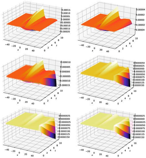
Figure 11. 3D plot of error of KdV–Burgers when $N=Nt=50,100$ (top: left to right), $N=Nt=200,300$ (middle: left to right) and $N=Nt=400,500$ (bottom: left to right).

14. A Case of KdV–Burgers’ Equation That Does Not Have an Exact Solution

In this section, a case of the KdV–Burgers’ equation whose exact solution is not known in the literature is considered. We use $\epsilon =0.2$, $\nu =0.2$ and $\mu =0.1$ with the initial condition [28]

$$u(x,0)=\frac{1}{2}\left(1-tanh\left(\frac{\left|x\right|-x_0}{d}\right)\right),$$

(67)

and boundary conditions

$$u_x(-50,t)=u_x(150,t)=u_{xx}(150,t)=0.$$

(68)

We solve the problem using the OCFE method with $N=300$ and compare the solution with the results obtained using the Mathematica v13.1 NDSolve built-in solver. We note that the value of $N=300$ is much smaller than the value of $N=4000$ used in [28]. The results are presented graphically in Figure 12 and Figure 13.

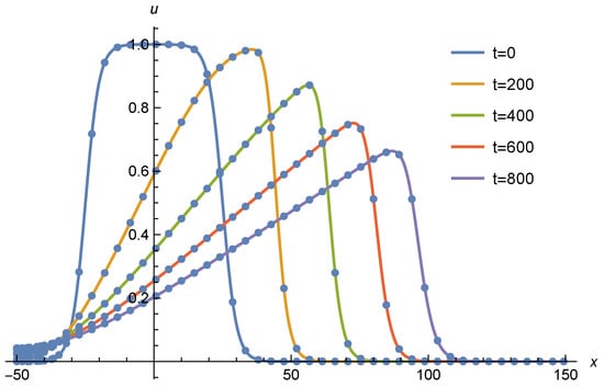
Figure 12. Comparison of OCFE solution (dots) and Mathematica built-in solver (solid line) at different times.

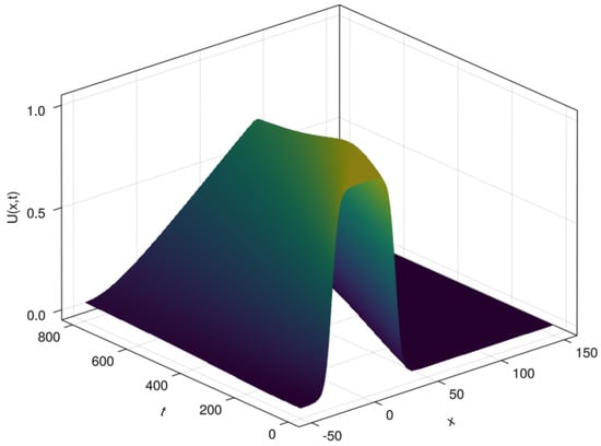
Figure 13. 3D plot for $N=300,t=800.$

The results in Figure 12 demonstrate that the OCFE method produces results which match the solution produced in Mathematica very closely.

15. Conclusions

We used the orthogonal collocation on finite elements method with quadratic B-spline and cubic spline bases to solve partial differential equations. In particular, Burgers’ equation was extensively explored to show the effectiveness of the method. It is easy to implement, unconditionally stable and convergent. Our results performed better than earlier results based on other forms of quadratic splines in the literature. We also demonstrated that the OCFE method is suitable for solving modified Burgers’ and KdV–Burgers’ equations.

In addition, a travelling wave solution of Burgers’ equation was considered in order to show the applicability of OCFE based on a quadratic B-spline basis. Velocity profiles were examined at various times and found to be consistent with existing results in the literature. Furthermore, we extended the OCFE method to cubic B-spline basis functions for solving third-order PDEs. This required two extra sets of equations to ensure that our solution is second-order continuously differentiable and requires three boundary conditions to solve the resulting system of linear equations. This method is suitable for differential equations of orders one to three and was used to find the solution of the KdV–Burgers’ equation. The approximate solution is highly accurate to second-order, both in time and space.

In conclusion, we found that orthogonal collocation based on quadratic and cubic B-spline bases performed well and produced accurate results that are second-order in time and space.

References

- Arora, S.; Kaur, I.; Tilahun, W. An exploration of quintic Hermite splines to solve Burgers’ equation. Arab. J. Math. 2020, 9, 19–36. [Google Scholar] [CrossRef]
- Botella, O.; Shariff, K. B-spline methods in fluid dynamics. Int. J. Comput. Fluid Dyn. 2003, 17, 133–149. [Google Scholar] [CrossRef]
- Singh, P.; Parumasur, N.; Bansilal, C. Orthogonal collocation on finite elements Using quintic Hermite basis. Aust. J. Math. Anal. Appl. 2021, 18, 1–12. [Google Scholar]
- Young, L.C. Orthogonal collocation revisited. Comput. Methods Appl. Mech. Engrg. 2019, 345, 1033–1076. [Google Scholar] [CrossRef]
- Biazar, J.; Ghazvini, H. Exact solutions for nonlinear Burgers’ equation by homotopy perturbation method. Numer. Methods Partial Differ. Equ. 2009, 25, 833–842. [Google Scholar] [CrossRef]
- Inc, M. On numerical solution of Burgers’ equation by homotopy analysis method. Phys. Lett. A 2008, 372, 356–360. [Google Scholar] [CrossRef]
- Hassanien, I.A.; Salama, A.A.; Hosham, H.A. Fourth-order finite difference method for solving Burgers’ equation. Appl. Math. Comput. 2005, 170, 781–800. [Google Scholar] [CrossRef]
- Zeidan, D.; Chau, C.K.; Lu, T.T.; Zheng, W.Q. Mathematical studies of the solution of Burgers’ equations by Adomian decomposition method. Math. Methods Appl. Sci. 2020, 43, 2171–2188. [Google Scholar] [CrossRef]
- Abbasbandy, S.; Darvishi, M.T. A numerical solution of Burgers’ equation by modified Adomian method. Appl. Math. Comput. 2005, 163, 1265–1272. [Google Scholar] [CrossRef]
- Moghimi, M.; Hejazi, F.S. Variational iteration method for solving generalized Burgers’–Fisher and Burgers’ Equations. Chaos Solit. Fractals 2007, 33, 1756–1761. [Google Scholar] [CrossRef]
- Hall, C.A.; Meyer, W.W. Optimal error bounds for cubic spline interpolation. J. Approx. Theory 1976, 16, 105–122. [Google Scholar] [CrossRef]
- Mittal, R.C.; Jain, R.K. Redefined cubic B-splines collocation method for solving convection–diffusion equations. Appl. Math. Model. 2012, 36, 5555–5573. [Google Scholar] [CrossRef]
- Bialecki, B.; Fairweather, G. Orthogonal spline collocation method for partial differential equations. J. Comput. Appl. Math. 2001, 128, 55–82. [Google Scholar] [CrossRef]
- Ali, A.H.A.; Gardner, G.A.; Gardner, L.R.T.A. Collocation Solution for Burgers’ Equation Using Cubic B-Spline Finite Elements. Comput. Methods Appl. Mech. Eng. 1992, 100, 325–337. [Google Scholar] [CrossRef]
- Arora, G.; Singh, B.K. Numerical solution of Burgers’ equation with modified cubic B-spline differential quadrature method. Appl. Math. Comput. 2013, 22, 166–177. [Google Scholar] [CrossRef]
- Bialecki, B.; Fisher, N. Maximum norm convergence analysis of extrapolated Crank-Nicolson orthogonal spline collocation for Burgers’ equation in one space variable. J. Differ. Equ. Appl. 2018, 24, 1621–1642. [Google Scholar] [CrossRef]
- Bialecki, B.; Fairweather, G.; Karageorghis, A.; Maack, J. A quadratic spline collocation method for the Dirichlet biharmonic problem. Numer. Algorithms 2020, 83, 165–199. [Google Scholar] [CrossRef]
- De Boor, C.; Swartz, B. Collocation at Gaussian points. SIAM J. Numer. Anal. 1973, 10, 582–606. [Google Scholar] [CrossRef]
- Khalifa, A.K.A.; Eilbeck, J.C. Collocation with quadratic and cubic splines. IMA J. Numer. Anal. 1982, 2, 111–121. [Google Scholar] [CrossRef]
- Soliman, A.A.; Raslan, K.R. Collocation Method Using Quadratic B-Spline for the Rlw Equation. Int. J. Comput. Math. 2001, 78, 399–412. [Google Scholar] [CrossRef]
- Kumari, A.; Kukreja, V. Error bounds for septic Hermite interpolation and its implementation to study modified Burgers’ equation. Numer. Algorithms 2022, 89, 1799–1821. [Google Scholar] [CrossRef]
- Irk, D. Sextic b-spline collocation method for the modified Burgers’ equation. Kybernetes 2009, 38, 1599–1620. [Google Scholar] [CrossRef]
- Bratsos, A.G.; Khaliq, A.Q. An exponential time differencing method of lines for the Burgers’ and the modified Burgers’ equations. Numer. Methods Partial Differ. Equ. 2018, 34, 2024–2039. [Google Scholar] [CrossRef]
- Ramadan, M.A.; El-Danaf, T.S. Numerical treatment for the modified Burgers’ equation. Math. Comput. Simul. 2005, 70, 90–98. [Google Scholar] [CrossRef]
- Lakshmi, C.; Awasthi, A. Robust numerical scheme for nonlinear modified Burgers’ equation. Int. J. Comput. Math. 2018, 95, 1910–1926. [Google Scholar] [CrossRef]
- Kaya, D. An application of the decomposition method for the KdVb equation. Appl. Math. Comput. 2004, 152, 279–288. [Google Scholar] [CrossRef]
- Soliman, A.A. A numerical simulation and explicit solutions of KdV- Burgers’ and Lax’s seventh-order KdV equations. Chaos Solit. Fractals 2006, 29, 294–302. [Google Scholar] [CrossRef]
- Zaki, S.I. A quintic B-spline finite elements scheme for the KdVB equation. Comput. Methods Appl. Mech. Engrg. 2000, 188, 121–134. [Google Scholar] [CrossRef]
- Helal, M.; Mehanna, M.S.A. Comparison between two different methods for solving KdV–Burgers’ equation. Chaos Solit. Fractals 2006, 28, 320–326. [Google Scholar] [CrossRef]
- Demiray, H. A note on the exact travelling wave solution to the KdV–Burgers’ equation. Wave Motion 2003, 38, 367–369. [Google Scholar] [CrossRef]
- Wang, M. Exact solutions for a compound KdV-Burgers’ equation. Phys. Lett. A 1996, 213, 279–287. [Google Scholar] [CrossRef]
- Jeffrey, A.; Mohamad, M.N. Exact solutions to the KdV-Burgers’ equation. Wave Motion 1991, 14, 369–375. [Google Scholar] [CrossRef]
- Wazzan, L.A. Modified Tanh–Coth method for solving the KdV and the KdV–Burgers’ equations. Commun. Nonlinear Sci. Numer. Simul. 2009, 14, 443–450. [Google Scholar] [CrossRef]
- Kudryashov, N.A. On new travelling wave solutions of the KdV and the KdV–Burgers’ equations. Commun. Nonlinear Sci. Numer. Simul. 2009, 14, 1891–1900. [Google Scholar] [CrossRef]
- Ramadan, M.A.; Aly, H.S. New approach for solving of extended KdV Equation. AJBAS 2023, 4, 96–109. [Google Scholar] [CrossRef]
- Raslan, K.R.A. Collocation solution for Burgers’ equation using quadratic B-spline finite elements. Int. J. Comput. Math. 2003, 80, 931–938. [Google Scholar] [CrossRef]
Disclaimer/Publisher’s Note: The statements, opinions and data contained in all publications are solely those of the individual author(s) and contributor(s) and not of MDPI and/or the editor(s). MDPI and/or the editor(s) disclaim responsibility for any injury to people or property resulting from any ideas, methods, instructions or products referred to in the content. |
© 2023 by the authors. Licensee MDPI, Basel, Switzerland. This article is an open access article distributed under the terms and conditions of the Creative Commons Attribution (CC BY) license (https://creativecommons.org/licenses/by/4.0/).