Modified Picard-like Method for Solving Absolute Value Equations

Abstract

We present a modified Picard-like method to solve absolute value equations by equivalently expressing the implicit fixed-point equation form of the absolute value equations as a two-by-two block nonlinear equation. This unifies some existing matrix splitting algorithms and improves the efficiency of the algorithm by introducing the parameter $\omega$. For the choice of $\omega$ in the new method, we give a way to determine the quasi-optimal values. Numerical examples are given to show the feasibility of the proposed method. It is also shown that the new method is better than those proposed by Ke and Ma in 2017 and Dehghan and Shirilord in 2020.

1. Introduction

The absolute value equation (AVE)

$$Ax-B\left|x\right|=b,$$

(1)

where $A\in {\mathbb{R}}^{n\times n}$, $B\in {\mathbb{R}}^{n\times n}$, $b\in {\mathbb{R}}^n$ and $\left|x\right|$=$\left(\right|x_1|,|x_2|,\dots ,|x_n{\left|\right)}^{\mathrm{T}}$, was introduced by Rohn [1], and has attracted the attention of many scholars, such as Mangasarian [2,3], Mangasarian and Meyer [4], Noor et al. [5,6,7], and Ketabchi and Moosaei [8,9,10,11], because it can be used as an important tool in the optimization field, such as in the complementarity problem, linear programming, and convex quadratic programming [12]. When $B=I$, (1) will become

$$Ax-\left|x\right|=b,$$

(2)

which can be obtained from a class of ordinary differential equations [5],

$$\frac{d^{2}x}{d{t}^2}-\left|x\right|=(a-t^2),0\le t\le 1.$$

Obviously, when B is the zero matrix, AVE (1) reduces to a linear system. In general, the matrix B in AVE (1) is supposed to be nonzero.

One of the important problems in the AVE is the existence and uniqueness of its solution. There are a variety of existence and uniqueness results; for instance, in [13], Rohn proved that if ${\sigma }_{max}\left(A^{-1}B\right)<1$ or ${\sigma }_{max}\left(\right|A^{-1}B\left|\right)<1$ (in this paper, we consider $\parallel A^{-1}B\parallel <1$, where $\parallel ·\parallel$ means the 2-norm), then AVE (1) has an unique solution for any $b\in {\mathbb{R}}^n$, where ${\sigma }_{max}(·)$ denotes the largest singular value of the matrices; in [14], Wu and Guo proved that if A can be expressed as $A=\beta I+M$, where $\beta \ge 1$, and M is a nonsingular M-matrix, then AVE (1) has an unique solution for any vector b; in addition, in [15], Wu and Li proved that AVE (1) has a unique solution for any vector b, if and only if matrix $A+I-2D$ is nonsingular for any diagonal matrix $D=\mathrm{diag}\left(d_i\right)$ with $0\le d_i\le 1$. We refer to [4,16] for other sufficient or necessary conditions for the existence and uniqueness results.

In this paper, we focus on another problem in the AVE (1), that is, how to solve the AVE (1). In fact, various numerical methods have been developed; for instance, Mangasarian, in [17], proposed a generalized Newton method for solving the AVE, which generated a sequence formally stated as

$$(A-D\left(x^{\left(k\right)}\right))x^{(k+1)}=b,$$

where the diagonal matrix $D\left(x\right):=\mathrm{diag}\left(\mathrm{sgn}\right(x\left)\right)$, $x\in {\mathbb{R}}^n$. It was proved to be convergent under certain conditions; Lian et al., in [18], further studied the generalized Newton method and obtained the weaker convergence results; Wang et al., in [19], proposed some modified Newton-type iteration methods for generalized absolute value equations. Since the convergence requirements of Newton’s method are strict, Edalatpour et al., in [20], proposed a generalization of the Gauss–Seidel iteration method; in addition, Ke and Ma, in [21], proposed an SOR-like iteration method by reformulating equivalently the AVE (1) as a two-by-two block nonlinear equation

$$\left\{\begin{array}{c}Ax-By=b,\hfill \\ -\left|x\right|+y=0.\hfill \end{array}\right.$$

(3)

Guo, Wu, and Li, in [22], presented some new convergence conditions obtained from the involved iteration matrix of the SOR-like iteration method in [21]; also based on (3), Li and Wu, in [23], improved the SOR-like iteration method proposed by Ke and Ma in [21] and obtained a modified SOR-like iteration method; Ali et al. proposed two modified generalized GaussSeidel (MGGS) iteration techniques to determine the AVE (1) in [24]. To accelerate the convergence, in [25], Salkuyeh proposed the Picard-HSS iteration method for the AVE; Zheng extended this method to the Picard-HSS-SOR Method in [26]; in [27], Ma proposed Picard methods for solving the AVE by combining matrix splitting iteration algorithms, such as the Jacobi, SSOR, or SAOR; Dehghan et al., in [28], proposed the following matrix multisplitting Picard-iterative methods (PIM), see Algorithm 1, under the condition ${\sigma }_{min}\left(A\right)>n{\sigma }_{max}\left(B\right)$. In addition, for A being an M-matrix case, in [29], Ali et al. presented two new generalized Gauss–Seidel iteration methods; finally, in [30], Yu et al. proposed an inverse-free dynamical system to solve AVE (1). We also refer to [8,9,10,14,25,31,32,33,34,35] for other methods of finding the solution to the AVE.

Algorithm 1:Picard Iteration Method (PIM).

Suppose that $x^{\left(0\right)}\in {\mathbb{R}}^n$ is an initial guess for the solution of (3), $ϵ$ is the target accuracy, and     $A=M_i-N_i$ ($i=$1, 2, …, p, where p is a positive integer) is a splitting for matrix A, where $M_i^{-1}$     exists. We compute $x^{(k+1)}\in {\mathbb{R}}^n$ by using the following iteration: 1. Input $x^{\left(0\right)}$; 2. Solve the following equations to obtain $x^{(k,t_k)}$, $k=0,1,2,\dots ,t=0,1,\dots ,t_k-1,$ where $t_k$     is a positive integer. $$\left\{\begin{array}{c}{x}^{(k,t+\frac{1}{p})}=M_1^{-1}{N}_1{x}^{(k,t)}+M_1^{-1}B\left|x^{\left(k\right)}\right|+M_1^{-1}b,\hfill \\ x^{(k,t+\frac{2}{p})}=M_2^{-1}{N}_2{x}^{(k,t+\frac{1}{p})}+M_2^{-1}B\left|x^{\left(k\right)}\right|+M_2^{-1}b,\hfill \\ x^{(k,t+\frac{3}{p})}=M_3^{-1}{N}_3{x}^{(k,t+\frac{2}{p})}+M_3^{-1}B\left|x^{\left(k\right)}\right|+M_3^{-1}b,\hfill \\ \dots ,\hfill \\ x^{(k,t+1)}=M_p^{-1}{N}_p{x}^{(k,t+1-\frac{1}{p})}+M_p^{-1}B\left|x^{\left(k\right)}\right|+M_p^{-1}b;\hfill \end{array}\right.$$ 3. Set $x^{(k+1)}=x^{(k,t_k)}$; 4. End the iteration when $\parallel b-A{x}^{(k+1)}+B|x^{(k+1)}|\parallel \le ϵ$; 5. Output $x^{(k+1)}$.

The main contributions of this paper are listed as follows.

(1) Based on a splitting of the two-by-two block coeffificient matrix, the Modified Picard-Like Iteration Method (MPIM) is proposed for solving AVE (1). It unifies some existing matrix splitting algorithms, such as the algorithms in [21,23,24,25,26,28];

(2) Compared with Algorithm 1, we introduce a parameter, $\omega$, to accelerate the convergence of the proposed MPIM method. The quasi-optimal parameters for the MPIM method are also given for various cases.

The present paper proceeds as follows. In Section 2, based on the equivalent form (3), we present a general matrix splitting method for solving the AVE (1). It unifies some existing matrix splitting methods. Furthermore, by combining this with the Picard technique, we propose an MPIM method. In Section 3, some numerical examples are given to show the feasibility and efficiency of the new methods.

2. Modified Picard-like Iteration Method

In this section, based on (3), we first give a general matrix splitting iteration method. By combining this with the Picard technique, we propose a Modified Picard-Like iteration method named MPIM. We also discuss the choice of the quasi-optimal parameter of the MPIM.

2.1. General Matrix Splitting Iteration

As stated in Section 1, by letting $y=\left|x\right|$, AVE (1) is equivalent to the form (3). Note that the matrix form for (3) can be written as $\widehat{A}\widehat{X}=\widehat{b}$, where

$$\widehat{A}=\left(\begin{array}{cc}A& -B\\ -D\left(x\right)& I\end{array}\right),\widehat{X}=\left(\begin{array}{c}x\\ y\end{array}\right),\widehat{b}=\left(\begin{array}{c}b\\ 0\end{array}\right),$$

and $x,y\in {\mathbb{R}}^n$. Hence, if we let $A=M-N$, and $M^{-1}$ exists, then $\widehat{A}=\widehat{M}-\widehat{N}$, where

$$\widehat{M}=\left(\begin{array}{cc}M& 0\\ -D\left(x\right)& {\omega }^{-1}I\end{array}\right),\widehat{N}=\left(\begin{array}{cc}N& B\\ 0& ({\omega }^{-1}-1)I\end{array}\right).$$

Furthermore, the form (3) can be reformulated as

$$\left(\begin{array}{c}x\\ y\end{array}\right)={\widehat{M}}^{-1}\widehat{N}\left(\begin{array}{c}x\\ y\end{array}\right)+{\widehat{M}}^{-1}\left(\begin{array}{c}b\\ 0\end{array}\right).$$

(4)

This provides an iteration method to solve AVE (1) as below, see Algorithm 2.

Algorithm 2:General Splitting Iteration Method (GSIM).

Suppose that $x^{\left(0\right)},y^{\left(0\right)}\in {\mathbb{R}}^n$ is an initial guess for the solution of (3), $ϵ$ is the target accuracy,     $\omega >0$, and $A=M-N$ is a splitting for matrix A. We compute $x^{(k+1)}\in {\mathbb{R}}^n$ by using the     following iteration: 1. Input $x^{\left(0\right)}$. 2. Solve the following equations to obtain $x^{(k+1)}$, $k=0,1,2,\dots$ $$\left\{\begin{array}{c}{x}^{(k+1)}=M^{-1}N{x}^{\left(k\right)}+M^{-1}B{y}^{\left(k\right)}+M^{-1}b,\hfill \\ y^{(k+1)}=\omega \left|x^{(k+1)}\right|+(1-\omega )y^{\left(k\right)}.\hfill \end{array}\right.$$ (5) 3. End the iteration when $\parallel b-A{x}^{(k+1)}+B|x^{(k+1)}|\parallel \le ϵ$. 4. Output $x^{(k+1)}$.

 Remark 1. 

The GSIM unifies some existing matrix splitting algorithms for the AVE. For example, if $M={\omega }^{-1}A$, and $B=I$, then it becomes the SOR-like method (SOR) proposed by Ma and Ke in [21]; if $M={\omega }^{-1}D-L$, and $B=I$, where $D=\mathrm{diag}\left(A\right)$, then it becomes the Modified SOR-like method (M-SOR) proposed by Wu and Li in [23]; if $M={\beta }^{-1}({\theta }^{-1}I+D-\lambda L),B=I$, and $\omega =1$, then it becomes the MGGS by Ali et al. in [24]; if $M=D$, then we obtain a new algorithm named the Modified Jacobi iteration method; if $M={\left[(2-\gamma )\gamma \right]}^{-1}[D-\gamma (L+U)+{\gamma }^{2}L{D}^{-1}U]$, then we obtain another new algorithm named the Modified SSOR-Like method (M-SSOR). It should be pointed out here that by choosing other splittings for the matrix A, more methods can be extracted.

Next, a theoretical analysis of the convergence for the GSIM is performed according to the following result, which can be found in [23].

 Lemma 1 

([23]). Let λ be any root of $x^2-bx+d=0$ with $b,d\in \mathbb{R}$. Then, $\left|\lambda \right|<1$, if and only if $\left|d\right|<1$, and $\left|b\right|<1+d$.

 Theorem 1. 

Let$A\in {\mathbb{R}}^{n\times n}$be nonsingular and$b\in {\mathbb{R}}^n$, B, M, N, and ω be defined as in Algorithm 2. Denote$P=M^{-1}N$, $Q=M^{-1}B$, $s=1-\omega$, and$L=\omega Q$.

If

$$\left\{\begin{array}{c}\parallel P\parallel \left|s\right|<1,\hfill \\ \parallel L\parallel <(1-|s\left|\right)(1-\parallel P\parallel ),\hfill \end{array}\right.$$

(6)

then

$${\displaystyle \underset{k\to +\infty }{lim}\parallel e_x^{\left(k\right)}\parallel =0,\underset{k\to +\infty }{lim}\parallel e_y^{\left(k\right)}\parallel =0,}$$

where

$$\left\{\begin{array}{c}{e}_x^{\left(k\right)}=x^{*}-x^{\left(k\right)},\hfill \\ e_y^{\left(k\right)}=y^{*}-y^{\left(k\right)},\hfill \end{array}\right.$$

(7)

where$(x^{*},y^{*})$is the solution pair of (4), and $(x^{\left(k\right)},y^{\left(k\right)})$ is generated by the iteration scheme (5).

 Proof. 

According to (5) and (7), we obtain

$$\left\{\begin{array}{c}{e}_x^{(k+1)}=P{e}_x^{\left(k\right)}+Q{e}_y^{\left(k\right)},\hfill \\ e_y^{(k+1)}=s{e}_y^{\left(k\right)}+\omega \left(\right|x^{*}|-|x^{(k+1)}\left|\right).\hfill \end{array}\right.$$

(8)

This implies

$$\parallel e_x^{(k+1)}\parallel \le \parallel P\parallel \parallel e_x^{\left(k\right)}\parallel +\parallel Q\parallel \parallel e_y^{\left(k\right)}\parallel ,$$

and

$$\parallel e_y^{(k+1)}\parallel \le \left|s\right|\parallel e_y^{\left(k\right)}\parallel +\left|\omega \right|\parallel \left(\right|x^{*}|-|x^{(k+1)}\left|\right)\parallel$$

$$\le \left|s\right|\parallel e_y^{\left(k\right)}\parallel +\left|\omega \right|\parallel x^{*}-x^{(k+1)}\parallel$$

$$=\left|s\right|\parallel e_y^{\left(k\right)}\parallel +\left|\omega \right|\parallel e_x^{(k+1)}\parallel .$$

Thus,

$$\left(\begin{array}{cc}-\omega & 1\\ 1& 0\end{array}\right)\left(\begin{array}{c}\parallel e_x^{(k+1)}\parallel \\ \parallel e_y^{(k+1)}\parallel \end{array}\right)\le \left(\begin{array}{cc}0& \left|s\right|\\ \parallel P\parallel & \parallel Q\parallel \end{array}\right)\left(\begin{array}{c}\parallel e_x^{\left(k\right)}\parallel \\ \parallel e_y^{\left(k\right)}\parallel \end{array}\right).$$

(9)

Since $\omega >0$, and the inverse of the matrix $\left(\begin{array}{cc}-\omega & 1\\ 1& 0\end{array}\right)$ is

$$\left(\begin{array}{cc}0& 1\\ 1& \omega \end{array}\right)>0,$$

by Inequality (9), we have

$$\left(\begin{array}{c}\parallel e_x^{(k+1)}\parallel \\ \parallel e_y^{(k+1)}\parallel \end{array}\right)\le \left(\begin{array}{cc}\parallel P\parallel & \parallel Q\parallel \\ \parallel \omega P\parallel & \left|s\right|+\parallel \omega Q\parallel \end{array}\right)\left(\begin{array}{c}\parallel e_x^{\left(k\right)}\parallel \\ \parallel e_y^{\left(k\right)}\parallel \end{array}\right)$$

$$\le {\left(\begin{array}{cc}\parallel P\parallel & \parallel Q\parallel \\ \parallel \omega P\parallel & \left|s\right|+\parallel \omega Q\parallel \end{array}\right)}^2\left(\begin{array}{c}\parallel e_x^{(k-1)}\parallel \\ \parallel e_y^{(k-1)}\parallel \end{array}\right)$$

                    …

$$\le {\left(\begin{array}{cc}\parallel P\parallel & \parallel Q\parallel \\ \parallel \omega P\parallel & \left|s\right|+\parallel \omega Q\parallel \end{array}\right)}^k\left(\begin{array}{c}\parallel e_x^{\left(0\right)}\parallel \\ \parallel e_y^{\left(0\right)}\parallel \end{array}\right).$$

Let

$$T=\left(\begin{array}{cc}\parallel P\parallel & \parallel Q\parallel \\ \parallel \omega P\parallel & \left|s\right|+\parallel \omega Q\parallel \end{array}\right).$$

Then, the spectral radius $\rho \left(T\right)=max\left\{\right|\lambda |:\lambda isaneigenvalueofT\}<1$. In fact, we assume that $\lambda$ is an eigenvalue of matrix T; then,

$$(\lambda -\parallel P\parallel )(\lambda -|s|-\parallel \omega Q\parallel )-\omega \parallel P\parallel \parallel Q\parallel =0,$$

which is equal to

$${\lambda }^2-\left(\right|s|+\omega \parallel Q\parallel +\parallel P\parallel )\lambda +\parallel P\parallel \left|s\right|=0.$$

(10)

By applying Lemma 1 to (10), $\lambda <1$ is equal to

$$\parallel P\parallel \left|s\right|<1,\parallel L\parallel <(1-|s\left|\right)(1-\parallel P\parallel ).$$

Therefore, $\rho \left(T\right)<1$; consequently,

$${\displaystyle \underset{k\to +\infty }{lim}\parallel e_x^{\left(k\right)}\parallel =0,\underset{k\to +\infty }{lim}\parallel e_y^{\left(k\right)}\parallel =0.}$$

The proof is complete.    □

Theorem 1 tells us that the iteration sequence $(x^{\left(k\right)},y^{\left(k\right)})$ produced by the GSIM can converge to the solution of (3) under some conditions. This also holds true for all the methods in Remark 1.

2.2. Modified Picard-like Iteration Method

In Section 2.1, if we increase some equations

$$x^{(k+1)}=M_i^{-1}{N}_i{x}^{\left(k\right)}+M_i^{-1}B{y}^{\left(k\right)}+M_i^{-1}b,i=1,2,3,\dots$$

(11)

in (5), then we obtain the MPIM.

 Remark 2. 

The MPIM unifies some existing Picard-like methods for the AVE. For example, if $M_1={\gamma }^{-1}D-L$, and $M_2={\gamma }^{-1}D-U$, where γ is a positive constant and $\omega =1$, then this method will reduce to the Picard-SSOR Method in [28]; if $M_1={\gamma }^{-1}(D-\mu L)$, and $M_2={\gamma }^{-1}(D-\mu U)$, where γ and μ are positive constants and $\omega =1$, then this method will reduce to the Picard-SAOR Method in [28]; if $M_1=\gamma I+H$, and $M_2=\gamma I+S$, where $H=\frac{1}{2}(A+A^H)$, $S=\frac{1}{2}(A-A^H)$, γ is a positive constant, and $\omega =1$, then this method will reduce to the Picard-HSS Method in [25]; if $M_1=\gamma I+H$, and $M_2=\gamma I+S$, where $H=\frac{1}{2}(A+A^H)$, $S=\frac{1}{2}(A-A^H)$, γ is a positive constant, and $\omega \in (0,2)$, then this method will reduce to the Picard-HSS-SOR Method in [26]. Obviously, by choosing other splittings for the matrix A, more methods can be also extracted.

Now, we consider the convergence of the MPIM. In fact, similar to the computation in [28], the (20) in Step 2 can be rewritten as

$$x^{(k+1)}={\mathsf{\Theta }}_p^{t_k}{x}^{\left(k\right)}+(I-{\mathsf{\Theta }}_p^{t_k})A^{-1}B{y}^{\left(k\right)}+(I-{\mathsf{\Theta }}_p^{t_k})A^{-1}b,$$

(12)

where ${\mathsf{\Theta }}_p={\prod }_{l=1}^p{M}_l^{-1}{N}_l$. Thus, the corresponding iteration matrix for the MPIM is

$${\widehat{M}}^{-1}\widehat{N}=\left(\begin{array}{cc}{\mathsf{\Theta }}_p^{t_k}& (I-{\mathsf{\Theta }}_p^{t_k})A^{-1}B\\ \omega D{\mathsf{\Theta }}_p^{t_k}& \omega D(I-{\mathsf{\Theta }}_p^{t_k})A^{-1}B+(1-\omega )I\end{array}\right).$$

(13)

We use the notations presented in Section 2.1, and set $P={\mathsf{\Theta }}_p^{t_k}$, $Q=(I-{\mathsf{\Theta }}_p^{t_k})A^{-1}B$, $s=1-\omega$, and $L=\omega Q$. Obviously, as with the GSIM, the MPIM is convergent if

$$\left\{\begin{array}{c}\parallel P\parallel \left|s\right|=\parallel {\mathsf{\Theta }}_p^{t_k}\parallel |1-\omega |<1,\hfill \\ \parallel L\parallel =\parallel \omega Q\parallel <(1-|1-\omega \left|\right)(1-\parallel {\mathsf{\Theta }}_p^{t_k}\parallel )=(1-|s\left|\right)(1-\parallel P\parallel ).\hfill \end{array}\right.$$

(14)

2.3. Range of $\omega$

As stated in [28], the PIM may not be convergent if the matrix A and B do not satisfy

$$n{\sigma }_{max}\left(B\right)<{\sigma }_{min}\left(A\right).$$

(15)

Next, we analyze in detail how to select $\omega$ such that the MPIM converges even when (15) does not hold.

 Theorem 2. 

Suppose

$$0<\parallel {\mathsf{\Theta }}_p^{t_k}\parallel <\frac{1-\parallel A^{-1}B\parallel }{1+\parallel A^{-1}B\parallel };$$

(16)

if$\omega \in (0,1)$, then (14) holds, i.e., the MPIM is convergent.

 Proof. 

Note that

$$\parallel {\mathsf{\Theta }}_p^{t_k}\parallel <\frac{1-\parallel A^{-1}B\parallel }{1+\parallel A^{-1}B\parallel }$$

implies

$$(1+\parallel {\mathsf{\Theta }}_p^{t_k}\parallel )\parallel A^{-1}B\parallel <1-\parallel {\mathsf{\Theta }}_p^{t_k}\parallel ,$$

and

$$\parallel (I-{\mathsf{\Theta }}_p^{t_k})A^{-1}B\parallel <\parallel (I-{\mathsf{\Theta }}_p^{t_k})\parallel \parallel A^{-1}B\parallel <(1+\parallel {\mathsf{\Theta }}_p^{t_k}\parallel )\parallel A^{-1}B\parallel .$$

Hence,

$$\parallel Q\parallel =\parallel (I-{\mathsf{\Theta }}_p^{t_k})A^{-1}B\parallel <1-\parallel {\mathsf{\Theta }}_p^{t_k}\parallel .$$

This means

$$\parallel L\parallel =\parallel \omega Q\parallel \le \left|\omega \right|\parallel Q\parallel <(1-|1-\omega \left|\right)(1-\parallel {\mathsf{\Theta }}_p^{t_k}\parallel )=(1-|s\left|\right)(1-\parallel P\parallel ),$$

since $\omega \in (0,1)$. Furthermore, because 

$$\frac{-2}{1-\parallel A^{-1}B\parallel }<0<\omega ,$$

we obtain

$$\frac{1-\parallel A^{-1}B\parallel }{1+\parallel A^{-1}B\parallel }<\frac{1}{1-\omega },$$

i.e.,

$$\parallel {\mathsf{\Theta }}_p^{t_k}\parallel <\frac{1}{1-\omega };$$

hence

$$\parallel P\parallel \left|s\right|<1.$$

Therefore, for $\omega \in (0,1)$, (16) implies (14). The proof is complete.    □

 Theorem 3. 

Suppose

$$0<\parallel {\mathsf{\Theta }}_p^{t_k}\parallel <\frac{2-\omega -\omega \parallel A^{-1}B\parallel }{2-\omega +\omega \parallel A^{-1}B\parallel };$$

(17)

if$\omega \in \left(1,\frac{2}{1+\parallel A^{-1}B\parallel }\right)$, then (14) holds, i.e., the MPIM is convergent.

 Proof. 

Note that (17) is equal to

$$\omega (1+\parallel {\mathsf{\Theta }}_p^{t_k}\parallel )\parallel A^{-1}B\parallel <2-\omega +(\omega -2)\parallel {\mathsf{\Theta }}_p^{t_k}\parallel ,$$

and

$$\parallel (I-{\mathsf{\Theta }}_p^{t_k})\parallel \parallel A^{-1}B\parallel \le (\parallel I\parallel +\parallel {\mathsf{\Theta }}_p^{t_k}\parallel )\parallel A^{-1}B\parallel =(1+\parallel {\mathsf{\Theta }}_p^{t_k}\parallel )\parallel A^{-1}B\parallel ;$$

hence,

$$\parallel \omega Q\parallel \le \left|\omega \right|\parallel Q\parallel \le \omega \parallel (I-{\mathsf{\Theta }}_p^{t_k})\parallel \parallel A^{-1}B\parallel <2-\omega +(\omega -2)\parallel {\mathsf{\Theta }}_p^{t_k}\parallel .$$

This means

$$\parallel L\parallel =\parallel \omega Q\parallel <(1-|1-\omega \left|\right)(1-\parallel {\mathsf{\Theta }}_p^{t_k}\parallel )=(1-|s\left|\right)(1-\parallel P\parallel ).$$

Furthermore, since $\omega <\frac{2}{1+\parallel A^{-1}B\parallel }<2$, we obtain $\frac{1}{\omega -1}>1$; hence,

$$\parallel {\mathsf{\Theta }}_p^{t_k}\parallel <\frac{2-\omega -\omega \parallel A^{-1}B\parallel }{2-\omega +\omega \parallel A^{-1}B\parallel }<1<\frac{1}{\omega -1},$$

which implies

$$\parallel P\parallel \left|s\right|<1.$$

Therefore, for $\omega \in \left(1,\frac{2}{1+\parallel A^{-1}B\parallel }\right)$, (17) implies (14). The proof is complete.    □

Theorems 2 and 3 tell us that if we split the matrix A such that (16) or (17) holds, then we can choose some $\omega \in \left(0,\frac{2}{1+\parallel A^{-1}B\parallel }\right)$, such that the corresponding vector sequence generated by (20) in the MPIM is convergent.

2.4. Quasi-Optimal Value of $\omega$

It can be seen from Section 2.3 that for a given $\omega \in \left(0,\frac{2}{1+\parallel A^{-1}B\parallel }\right)$, we can always adopt a specific splitting form to make the algorithm converge. Next, we consider how to select $\omega$ to make the algorithm converge faster when the splitting form of the matrix has been given. For the MPIM, the iteration matrix

$${\widehat{M}}^{-1}\widehat{N}=\left(\begin{array}{cc}{\mathsf{\Theta }}_p^{t_k}& (I-{\mathsf{\Theta }}_p^{t_k})A^{-1}B\\ \omega D{\mathsf{\Theta }}_p^{t_k}& \omega D(I-{\mathsf{\Theta }}_p^{t_k})A^{-1}B+(1-\omega )I\end{array}\right)$$

$$=\left(\begin{array}{cc}I& 0\\ \omega D& I\end{array}\right)\left(\begin{array}{cc}{\mathsf{\Theta }}_p^{t_k}& (I-{\mathsf{\Theta }}_p^{t_k})A^{-1}B\\ 0& (1-\omega )I\end{array}\right)$$

$$=\left(\left(\begin{array}{cc}I& 0\\ 0& I\end{array}\right)+\left(\begin{array}{cc}0& 0\\ \omega D& 0\end{array}\right)\right)\left(\left(\begin{array}{cc}{\mathsf{\Theta }}_p^{t_k}& 0\\ 0& (1-\omega )I\end{array}\right)+\left(\begin{array}{cc}0& (I-{\mathsf{\Theta }}_p^{t_k})A^{-1}B\\ 0& 0\end{array}\right)\right).$$

Then,

$$\parallel {\widehat{M}}^{-1}\widehat{N}\parallel \le (1+\omega )\parallel \left(\begin{array}{cc}{\mathsf{\Theta }}_p^{t_k}& 0\\ 0& (1-\omega )I\end{array}\right)+\left(\begin{array}{cc}0& (I-{\mathsf{\Theta }}_p^{t_k})A^{-1}B\\ 0& 0\end{array}\right)\parallel$$

$$\le (1+\omega )\left(max\left\{|1-\omega |,\parallel {\mathsf{\Theta }}_p^{t_k}\parallel \right\}+\parallel (I-{\mathsf{\Theta }}_p^{t_k})A^{-1}B\parallel \right)$$

$$\le (1+\omega )\left(max\left\{|1-\omega ,|\parallel {\mathsf{\Theta }}_p^{t_k}\parallel \right\}+(1+\parallel {\mathsf{\Theta }}_p^{t_k}\parallel )\parallel A^{-1}B\parallel \right).$$

We denote

$$f(\omega ,\parallel {\mathsf{\Theta }}_p^{t_k}\parallel )=(1+\omega )\left(max\left\{|1-\omega |,\parallel {\mathsf{\Theta }}_p^{t_k}\parallel \right\}+(1+\parallel {\mathsf{\Theta }}_p^{t_k}\parallel )\parallel A^{-1}B\parallel \right).$$

(18)

Then,

$$\parallel {\widehat{M}}^{-1}\widehat{N}\parallel \le f(\omega ,\parallel {\mathsf{\Theta }}_p^{t_k}\parallel ).$$

(19)

Apparently, $\parallel {\widehat{M}}^{-1}\widehat{N}\parallel$ and $f(\omega ,\parallel {\mathsf{\Theta }}_p^{t_k}\parallel )$ all involve the $\omega$ and ${\mathsf{\Theta }}_p^{t_k}$. It is well known that the smaller $\parallel {\widehat{M}}^{-1}\widehat{N}\parallel$ is, the faster the MPIM converges. However, it is not easy to determine $\parallel {\widehat{M}}^{-1}\widehat{N}\parallel$ in general. So, we next discuss the minimum of $f(\omega ,\parallel {\mathsf{\Theta }}_p^{t_k}\parallel )$ instead of $\parallel {\widehat{M}}^{-1}\widehat{N}\parallel$ to provide some choices for $\omega$.

 Theorem 4. 

Suppose that $\parallel {\mathsf{\Theta }}_p^{t_k}\parallel$ is given with

$$\parallel {\mathsf{\Theta }}_p^{t_k}\parallel <\frac{1-\parallel A^{-1}B\parallel }{1+\parallel A^{-1}B\parallel }and0<\omega \le 1-\parallel {\mathsf{\Theta }}_p^{t_k}\parallel ;$$

then,

$$\underset{\omega \in (0,{\omega }_1]}{min}f(\omega ,\parallel {\mathsf{\Theta }}_p^{t_k}\parallel )=f({\omega }_1,\parallel {\mathsf{\Theta }}_p^{t_k}\parallel ),$$

where ${\omega }_1=1-\parallel {\mathsf{\Theta }}_p^{t_k}\parallel$.

Proof. 

Based on (18), when

$$0<\omega \le 1-\parallel {\mathsf{\Theta }}_p^{t_k}\parallel ,$$

we obtain

$$f(\omega ,\parallel {\mathsf{\Theta }}_p^{t_k}\parallel )=-{\omega }^2+(1+\parallel {\mathsf{\Theta }}_p^{t_k}\parallel )\parallel A^{-1}B\parallel \omega +(1+\parallel {\mathsf{\Theta }}_p^{t_k}\parallel )\parallel A^{-1}B\parallel +1.$$

Then, the axis of symmetry of the parabola is

$$\frac{(1+\parallel {\mathsf{\Theta }}_p^{t_k}\parallel )\parallel A^{-1}B\parallel }{2}.$$

We notice that

$$\parallel {\mathsf{\Theta }}_p^{t_k}\parallel <\frac{1-\parallel A^{-1}B\parallel }{1+\parallel A^{-1}B\parallel }.$$

This leads to

$$1-\parallel {\mathsf{\Theta }}_p^{t_k}\parallel -\frac{(1+\parallel {\mathsf{\Theta }}_p^{t_k}\parallel )\parallel A^{-1}B\parallel }{2}>\frac{(1+\parallel {\mathsf{\Theta }}_p^{t_k}\parallel )\parallel A^{-1}B\parallel }{2}-0,$$

i.e.,

$$\underset{\omega \in (0,{\omega }_1]}{min}f(\omega ,\parallel {\mathsf{\Theta }}_p^{t_k}\parallel )=f({\omega }_1,\parallel {\mathsf{\Theta }}_p^{t_k}\parallel ),$$

since the axis of symmetry of the parabola is $\frac{(1+\parallel {\mathsf{\Theta }}_p^{t_k}\parallel )\parallel A^{-1}B\parallel }{2}$. The proof is complete.    □

 Theorem 5. 

Suppose that$\parallel {\mathsf{\Theta }}_p^{t_k}\parallel$is given,$\omega \ge 1$, and (17) holds.

(I) If

$$\parallel {\mathsf{\Theta }}_p^{t_k}\parallel \in \left(\frac{1-\sqrt{\parallel A^{-1}B\parallel }}{1+\sqrt{\parallel A^{-1}B\parallel }},\frac{1-\parallel A^{-1}B\parallel }{1+\parallel A^{-1}B\parallel }\right),$$

then

$$\omega <{\omega }_{2}and\underset{\omega \in [1,{\omega }_2)}{min}f(\omega ,\parallel {\mathsf{\Theta }}_p^{t_k}\parallel )=f(1,\parallel {\mathsf{\Theta }}_p^{t_k}\parallel ),$$

where ${\omega }_2=1+\parallel {\mathsf{\Theta }}_p^{t_k}\parallel$.

(II) If

$$\parallel {\mathsf{\Theta }}_p^{t_k}\parallel \in \left(0,\frac{1-\sqrt{\parallel A^{-1}B\parallel }}{1+\sqrt{\parallel A^{-1}B\parallel }}\right),$$

then

$${\omega }_2\le \omega <{\omega }_{3}and\underset{\omega \in [{\omega }_2,{\omega }_3)}{min}f(\omega ,\parallel {\mathsf{\Theta }}_p^{t_k}\parallel )=f({\omega }_2,\parallel {\mathsf{\Theta }}_p^{t_k}\parallel ),$$

where ${\omega }_3=\frac{2-2\parallel {\mathsf{\Theta }}_p^{t_k}\parallel }{\parallel A^{-1}B\parallel \parallel {\mathsf{\Theta }}_p^{t_k}\parallel -\parallel {\mathsf{\Theta }}_p^{t_k}\parallel +\parallel A^{-1}B\parallel +1}$.

Proof. 

From (17), we obtain

$$\omega <\frac{2-2\parallel {\mathsf{\Theta }}_p^{t_k}\parallel }{\parallel A^{-1}B\parallel \parallel {\mathsf{\Theta }}_p^{t_k}\parallel -\parallel {\mathsf{\Theta }}_p^{t_k}\parallel +\parallel A^{-1}B\parallel +1}.$$

Since $\omega \ge 1$, we have

$$\frac{2-2\parallel {\mathsf{\Theta }}_p^{t_k}\parallel }{\parallel A^{-1}B\parallel \parallel {\mathsf{\Theta }}_p^{t_k}\parallel -\parallel {\mathsf{\Theta }}_p^{t_k}\parallel +\parallel A^{-1}B\parallel +1}>1,$$

i.e.,

$$\parallel {\mathsf{\Theta }}_p^{t_k}\parallel \in (0,\frac{1-\parallel A^{-1}B\parallel }{1+\parallel A^{-1}B\parallel }).$$

(I) Since

$$\frac{1-\sqrt{\parallel A^{-1}B\parallel }}{1+\sqrt{\parallel A^{-1}B\parallel }}<\frac{1-\parallel A^{-1}B\parallel }{1+\parallel A^{-1}B\parallel }<1<\frac{1+\sqrt{\parallel A^{-1}B\parallel }}{1-\sqrt{\parallel A^{-1}B\parallel }},$$

then

$$\parallel {\mathsf{\Theta }}_p^{t_k}\parallel \in \left(\frac{1-\sqrt{\parallel A^{-1}B\parallel }}{1+\sqrt{\parallel A^{-1}B\parallel }},\frac{1-\parallel A^{-1}B\parallel }{1+\parallel A^{-1}B\parallel }\right)\subset \left(\frac{1-\sqrt{\parallel A^{-1}B\parallel }}{1+\sqrt{\parallel A^{-1}B\parallel }},\frac{1+\sqrt{\parallel A^{-1}B\parallel }}{1-\sqrt{\parallel A^{-1}B\parallel }}\right).$$

Note that

$$\parallel {\mathsf{\Theta }}_p^{t_k}\parallel \in \left(\frac{1-\sqrt{\parallel A^{-1}B\parallel }}{1+\sqrt{\parallel A^{-1}B\parallel }},\frac{1+\sqrt{\parallel A^{-1}B\parallel }}{1-\sqrt{\parallel A^{-1}B\parallel }}\right)$$

is equal to

$$(1-\parallel A^{-1}B\parallel )\parallel {\mathsf{\Theta }}_p^{t_k}{\parallel }^2-(2\parallel A^{-1}B\parallel +2)\parallel {\mathsf{\Theta }}_p^{t_k}\parallel +1-\parallel A^{-1}B\parallel <0,$$

which means

$$\frac{2-2\parallel {\mathsf{\Theta }}_p^{t_k}\parallel }{\parallel A^{-1}B\parallel \parallel {\mathsf{\Theta }}_p^{t_k}\parallel -\parallel {\mathsf{\Theta }}_p^{t_k}\parallel +\parallel A^{-1}B\parallel +1}-1<\parallel {\mathsf{\Theta }}_p^{t_k}\parallel ,$$

i.e., $\omega <1+\parallel {\mathsf{\Theta }}_p^{t_k}\parallel$. So,

$$f(\omega ,\parallel {\mathsf{\Theta }}_p^{t_k}\parallel )=(1+\omega )(\parallel {\mathsf{\Theta }}_p^{t_k}\parallel +(1+\parallel {\mathsf{\Theta }}_p^{t_k}\parallel )\parallel A^{-1}B\parallel );$$

then,

$$\underset{\omega \in [1,{\omega }_2)}{min}f(\omega ,\parallel {\mathsf{\Theta }}_p^{t_k}\parallel )=f(1,\parallel {\mathsf{\Theta }}_p^{t_k}\parallel ).$$

(II) From (I), we know when

$$\parallel {\mathsf{\Theta }}_p^{t_k}\parallel \in \left(0,\frac{1-\sqrt{\parallel A^{-1}B\parallel }}{1+\sqrt{\parallel A^{-1}B\parallel }}\right),$$

we have $\omega \ge 1+\parallel {\mathsf{\Theta }}_p^{t_k}\parallel$, i.e.

$$\omega \in \left[1+\parallel {\mathsf{\Theta }}_p^{t_k}\parallel ,\frac{2-2\parallel {\mathsf{\Theta }}_p^{t_k}\parallel }{\parallel A^{-1}B\parallel \parallel {\mathsf{\Theta }}_p^{t_k}\parallel -\parallel {\mathsf{\Theta }}_p^{t_k}\parallel +\parallel A^{-1}B\parallel +1}\right).$$

Thus,

$$f(\omega ,\parallel {\mathsf{\Theta }}_p^{t_k}\parallel )=(1+\omega )\left(\omega -1+(1+\parallel {\mathsf{\Theta }}_p^{t_k}\parallel )\parallel A^{-1}B\parallel \right)$$

$$={\omega }^2+(1+\parallel {\mathsf{\Theta }}_p^{t_k}\parallel )\parallel A^{-1}B\parallel \omega +(1+\parallel {\mathsf{\Theta }}_p^{t_k}\parallel )\parallel A^{-1}B\parallel -1.$$

Similar to the proof of Theorem 4, we obtain

$$\underset{\omega \in [{\omega }_2,{\omega }_3)}{min}f(\omega ,\parallel {\mathsf{\Theta }}_p^{t_k}\parallel )=f({\omega }_2,\parallel {\mathsf{\Theta }}_p^{t_k}\parallel ).$$

The proof is complete.    □

It can be seen under the condition of Theorem 4 that we can choose an appropriate parameter $\omega$ to accelerate the convergence of the algorithm, even though the PIM does not converge, as shown in Section 3.2. Based on Theorem 5 (II), it can be seen that when

$$\parallel {\mathsf{\Theta }}_p^{t_k}\parallel \in \left(\frac{1-\sqrt{\parallel A^{-1}B\parallel }}{1+\sqrt{\parallel A^{-1}B\parallel }},\frac{1-\parallel A^{-1}B\parallel }{1+\parallel A^{-1}B\parallel }\right),$$

$f(\omega ,\parallel {\mathsf{\Theta }}_p^{t_k}\parallel )$ becomes a linear function, and the rate of convergence is almost completely determined by the value of $\parallel {\mathsf{\Theta }}_p^{t_k}\parallel$. It means under this condition, $\parallel {\mathsf{\Theta }}_p^{t_k}\parallel$ plays a more important role than $\omega$, and if we change the value of $\omega$, it will not cause great changes in the convergence, as shown in Section 3.2. Based on Theorem 5 (I), it also can be seen that when

$$\parallel {\mathsf{\Theta }}_p^{t_k}\parallel \in \left(0,\frac{1-\sqrt{\parallel A^{-1}B\parallel }}{1+\sqrt{\parallel A^{-1}B\parallel }}\right),$$

we can choose an appropriate parameter $\omega$ to accelerate the convergence of the algorithm, as shown in Section 3.2.

3. Numerical Examples

In this section, we demonstrate the performance of Algorithms 1–3 with numerical examples.

The numerical experiments were performed using MATLAB software on an Intel (R) Pentium (R) CPU N3700 for (1.60 GHz, 4 GB RAM). Zero vector $x^{\left(0\right)}=0$ was used for the initial guess. The iterations were terminated when the current iterate satisfied

$$\parallel Re\left(k\right)\parallel \le {10}^{-8},$$

where $\parallel Re\left(k\right)\parallel =\parallel b-A{x}^{\left(k\right)}+B|x^{\left(k\right)}{|\parallel }_{\infty }$ is the k-th iterate for the PIM, GSIM, and MPIM algorithms. For all mesh sizes m and n, we set $p=2$, and the max iteration was $=500$ in all the methods. Moreover, we took the vector b such that the solution $x={(-\frac{n}{2}+1:\frac{n}{2})}^{\mathrm{T}}$. For the matrices A and B, we took

$$A=T_x\otimes I_m+I_m\otimes T_y+200I_n,B=I,$$

in the GSIM algorithm, with tridiagonal matrices

$$T_x=Tridiagonal{(-1,4,-1)}_{l\times l}$$

and

$$T_y=Tridiagonal{(-1,0,-1)}_{l\times l},$$

where m and n are positive integer numbers, and ⊗ is the Kronecker product, where $l=10$. In addition, we took

$$A=T_x\otimes I_m+I_m\otimes T_y+320I_{n}andB=50i{I}_n+2I_m\otimes T_y,$$

in the PIM and MPIM algorithms to compare the efficiency of these methods, where $m=50,l=20,n=1000$, and $i=1,2,3,4,5,6$.

Algorithm 3:Modified Picard-Like Iteration Method (MPIM).

Suppose that $x^{\left(0\right)},y^{\left(0\right)}\in {\mathbb{R}}^n$ is an initial guess for solution of (3), $ϵ$ is the target accuracy, $\omega >0$, and $A=M_i-N_i$ ($i=$1, 2, …, p) is a splitting for matrix A, where $M_i^{-1}$ exists. We compute $x^{(k+1)}\in {\mathbb{R}}^n$ by using the following iteration: 1. Input $x^{\left(0\right)}$. 2. Solve the following equations to obtain $x^{(k,t_k)}$, $k=0,1,2,\dots ,t=0,1,\dots ,t_k-1$ $$\left\{\begin{array}{c}{x}^{(k,t+\frac{1}{p})}=M_1^{-1}{N}_1{x}^{(k,t)}+M_1^{-1}B{y}^{\left(k\right)}+M_1^{-1}b,\hfill \\ x^{(k,t+\frac{2}{p})}=M_2^{-1}{N}_2{x}^{(k,t+\frac{1}{p})}+M_2^{-1}B{y}^{\left(k\right)}+M_2^{-1}b,\hfill \\ x^{(k,t+\frac{3}{p})}=M_3^{-1}{N}_3{x}^{(k,t+\frac{2}{p})}+M_3^{-1}B{y}^{\left(k\right)}+M_3^{-1}b,\hfill \\ \dots ,\hfill \\ x^{(k,t+1)}=M_p^{-1}{N}_p{x}^{(k,t+1-\frac{1}{p})}+M_p^{-1}B{y}^{\left(k\right)}+M_p^{-1}b.\hfill \end{array}\right.$$ (20) 3. Set $x^{(k+1)}=x^{(k,t_k)}$. 4. Set $y^{(k+1)}=\omega \left|x^{(k+1)}\right|+(1-\omega )y^{\left(k\right)}$. 5. End the iteration when $\parallel b-A{x}^{(k+1)}+B|x^{(k+1)}|\parallel \le ϵ$. 6. Output $x^{(k+1)}$.

3.1. An Application

We solved the following ordinary differential equations:

$$\frac{d^{2}x}{d{t}^2}-\left|x\right|=(1-t^2),0\le t\le 1,x\left(0\right)=-1,x\left(1\right)=0,$$

to show our method is feasible. Similarly to the Example 3.1 in [5], we discredite the above equation using the finite difference method to obtain (2), where A of size 10 is given by:

$$a_{i,j}=\left\{\begin{array}{c}-242,forj=i,\hfill \\ 121,for\left\{\begin{array}{c}j=i+1,i=1,2,\dots ,9,\hfill \\ j=i-1,i=2,3,\dots ,10,\hfill \end{array}\right.\hfill \\ 0,otherwise,\hfill \end{array}\right.$$

and the exact solution is

$$x=-1.4621171757e^{-t}-0.5378828428e^t+1+t^2,t>0.$$

We compared the SOR algorithm with $\omega =0.5$, the M-SOR with $w=0.5$, and the MPIM with $M_1=2A$, $M_2=1.2A$, and $\omega =1.1$ to solve the above AVE problem in 72, 2156, and 18 iterations, respectively; see Figure 1.

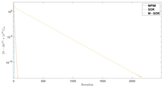
Figure 1. Number of iterations.

3.2. General Splitting Iteration Method

We solved (2), where A and B are as mentioned above, by Algorithm 2 and 3 with the following special methods: the SOR-like (SOR), the Modified SOR-Like (M-SOR), and the Modified SSOR-Like (M-SSOR) with $\gamma =\omega =0.5$, the Modified Picard-SSOR (MP-SSOR) with $\omega =1.05$ and $\gamma =0.5$, and the MGGS with $\beta =0.5$, $\theta =0.2$ and $\lambda =0.8$; see Remarks 1 and 2.

From Table 1, we can see that when $B=I,$ the M-SSOR and MP-SSOR proposed in this paper were better than the previous algorithms [21,23,24]. Note that for all the iterative methods, we did not choose the best parameters of $\omega$ to further optimize the algorithm (in fact, the splitting parameter of A can be different from $\omega$ to speed up the algorithm, as discussed in Remark 2).

Table 1. Comparision of the iteration number and the CPU time in (2).

n	500	1000	2000	3000	4000	5000	6000
SOR
Iteration	46	47	48	49	49	50	50
CPU Time(s)	0.022361	0.085864	0.314504	0.825014	1.347516	2.122693	2.866091
$\parallel RE\left(k\right)\parallel$	$7.28\times {10}^{-9}$	$7.62\times {10}^{-9}$	$8.02\times {10}^{-9}$	$6.37\times {10}^{-9}$	$8.46\times {10}^{-9}$	$6.43\times {10}^{-9}$	$7.07\times {10}^{-9}$
MGGS
Iteration	46	47	48	48	49	49	49
CPU Time(s)	0.022301	0.090165	0.304298	0.844811	1.342616	2.120393	2.796891
$\parallel RE\left(k\right)\parallel$	$5.12\times {10}^{-9}$	$5.25\times {10}^{-9}$	$5.34\times {10}^{-9}$	$8.17\times {10}^{-9}$	$5.45\times {10}^{-9}$	$7.23\times {10}^{-9}$	$8.07\times {10}^{-9}$
M-SOR
Iteration	47	48	49	50	50	51	51
CPU Time(s)	0.022223	0.082626	0.304649	0.783727	1.381016	2.1367	2.979601
$\parallel RE\left(k\right)\parallel$	$6.79\times {10}^{-9}$	$7.70\times {10}^{-9}$	$8.77\times {10}^{-9}$	$7.07\times {10}^{-9}$	$9.56\times {10}^{-9}$	$6.43\times {10}^{-9}$	$7.76\times {10}^{-9}$
M-SSOR
Iteration	39	40	41	41	42	42	42
CPU Time(s)	0.020607	0.072805	0.290216	0.634203	1.089738	1.692161	2.458237
$\parallel RE\left(k\right)\parallel$	$5.75\times {10}^{-9}$	$5.85\times {10}^{-9}$	$5.94\times {10}^{-9}$	$8.92\times {10}^{-9}$	$6.14\times {10}^{-9}$	$7.82\times {10}^{-9}$	$9.61\times {10}^{-9}$
MP-SSOR
$t_k$	2	2	2	2	2	2	2
Iteration	13	13	13	13	13	13	13
CPU Time(s)	0.01634	0.06855	0.232589	0.559356	0.993672	1.586937	2.206395
$\parallel RE\left(k\right)\parallel$	$8.46\times {10}^{-9}$	$1.40\times {10}^{-9}$	$2.95\times {10}^{-9}$	$4.58\times {10}^{-9}$	$6.08\times {10}^{-9}$	$7.76\times {10}^{-9}$	$9.50\times {10}^{-9}$

3.3. Modified Picard-like Iteration Method

Moreover, we solved (1) by the MPIM and PIM with special splitting ($M_3=0.5D-L$, $M_4=1.5D-U$, record as a splitting 1). Since

$$\parallel {\mathsf{\Theta }}_p^{t_k}\parallel <\frac{1-\parallel A^{-1}B\parallel }{1+\parallel A^{-1}B\parallel },$$

based on Theorem 4, we chose $\omega ={\omega }_1=1-\parallel {\mathsf{\Theta }}_p^{t_k}\parallel \approx 0.66$. Some numerical results, such as the number of iterations, the parameters $\omega$, the CPU time needed to run the iterative methods, and the residual error Re(k), are reported in Table 2.

Table 2. Comparision of the iteration number and the CPU time for $M_i$, $i=3,4$.

i	1	2	3	4	5	6
PIM
$t_k$	1	1	1	1	1	1
Iteration	51	106	500	500	500	500
CPU Time(s)	0.245599	0.514312	2.329751	2.329751	2.329751	2.329751
$\parallel Re\left(k\right)\parallel$	$5.9590\times {10}^{-9}$	$7.7489\times {10}^{-9}$	$4.0375\times {10}^{-4}$	NAN	NAN	NAN
MPIM
$\omega$	0.66	0.66	0.66	0.66	0.66	0.66
$t_k$	1	1	1	1	1	1
Iteration	36	46	61	90	155	483
CPU Time(s)	0.186891	0.226695	0.285497	0.433709	0.723879	2.240295
$\parallel Re\left(k\right)\parallel$	$4.9986\times {10}^{-9}$	$5.1004\times {10}^{-9}$	$8.8476\times {10}^{-9}$	$7.1886\times {10}^{-9}$	$8.2655\times {10}^{-9}$	$9.9244\times {10}^{-9}$

From Table 2, we can see that with the increase in i, i.e., the increase in the maximum singular value of B, the Picard method gradually tended to be non-convergent for a given splitting form. However, when we took $\omega ={\omega }_1\approx 0.66$, the algorithm was always convergent. This is consistent with the analysis of Theorem 4. When $B=50I_{1000}+2I_{50}\otimes T_{20}$, the spectral radius of iterative matrix ${\widehat{M}}^{-1}\widehat{N}$ was recorded as $\rho \left({\widehat{M}}^{-1}\widehat{N}\right)$ in Figure 2, where

$${\omega }_3=\frac{2-2\parallel {\mathsf{\Theta }}_p^{t_k}\parallel }{\parallel A^{-1}B\parallel \parallel {\mathsf{\Theta }}_p^{t_k}\parallel -\parallel {\mathsf{\Theta }}_p^{t_k}\parallel +\parallel A^{-1}B\parallel +1}\approx 1.49.$$

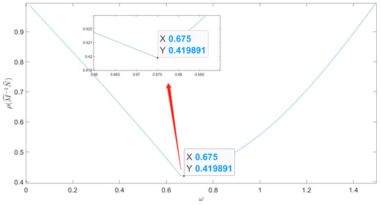
Figure 2. The spectral radius of ${\widehat{M}}^{-1}\widehat{N}$ for $M_i$, $i=3,4$.

In addition, we changed the spliiting of A. For the PIM and MPIM, we let $M_5={\gamma }^{-1}D-L$, and $M_6={\gamma }^{-1}D-U$, where $\gamma =1.5$. Since

$$\parallel {\mathsf{\Theta }}_p^{t_k}\parallel \in \left(0,\frac{1-\sqrt{\parallel A^{-1}B\parallel }}{1+\sqrt{\parallel A^{-1}B\parallel }}\right),$$

based on Theorem 5 (II), we chose $\omega ={\omega }_2=1+\parallel {\mathsf{\Theta }}_p^{t_k}\parallel \approx 1.28$, where

$$B=50\times 1\times I_{1000}+2I_{50}\otimes T_{20}.$$

It can be seen from Table 3 that when the splitting form was modified, the MPIM was still better than the PIM. We selected $B=50I_{1000}+2I_{50}\otimes T_{20}$ to give the spectral radius under different $\omega$ values, as shown in Figure 3, where

$${\omega }_3=\frac{2-2\parallel {\mathsf{\Theta }}_p^{t_k}\parallel }{\parallel A^{-1}B\parallel \parallel {\mathsf{\Theta }}_p^{t_k}\parallel -\parallel {\mathsf{\Theta }}_p^{t_k}\parallel +\parallel A^{-1}B\parallel +1}\approx 1.54.$$

Table 3. Comparision of the iteration number and the CPU time for $M_i$, $i=5,6$.

i	1	2	3	4	5	6
PIM
$t_k$	1	1	1	1	1	1
Iteration	31	42	58	87	153	500
CPU Time(s)	0.145542	0.186529	0.257494	0.396560	0.692243	2.372002
$\parallel Re\left(k\right)\parallel$	$6.8540\times {10}^{-9}$	$6.5775\times {10}^{-9}$	$8.8039\times {10}^{-9}$	$8.8912\times {10}^{-9}$	$9.6479\times {10}^{-9}$	$1.0696\times {10}^{-8}$
MPIM
$\omega$	1.28	1.1	1.1	1.1	1.1	1.1
$t_k$	1	1	1	1	1	1
Iteration	30	40	55	81	143	467
CPU Time(s)	0.137961	0.168187	0.230488	0.350071	0.613298	2.014428
$\parallel Re\left(k\right)\parallel$	$5.9881\times {10}^{-9}$	$4.7221\times {10}^{-9}$	$5.9517\times {10}^{-9}$	$9.0949\times {10}^{-9}$	$8.6729\times {10}^{-9}$	$9.7934\times {10}^{-9}$

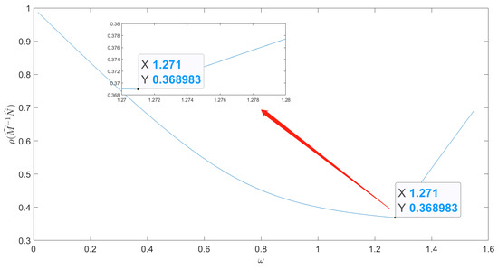
Figure 3. The spectral radius of ${\widehat{M}}^{-1}\widehat{N}$ for $M_i$, $i=5,6$.

Now, for the MPIM and the PIM, we chose $M_7={\gamma }^{-1}D-L,M_8={\gamma }^{-1}D-U$, and $t_k=2$, where $\gamma =1.8$, record as a splitting 3. We selected $B=50I_{1000}+2I_{50}\otimes T_{20}$ to give the spectral radius under different $\omega$ values, as shown in Figure 4. Since

$$\parallel {\mathsf{\Theta }}_p^{t_k}\parallel \in \left(\frac{1-\sqrt{\parallel A^{-1}B\parallel }}{1+\sqrt{\parallel A^{-1}B\parallel }},\frac{1-\parallel A^{-1}B\parallel }{1+\parallel A^{-1}B\parallel }\right),$$

based on Theorem 5 (I), we chose $\omega =1$. Then, we see that when $\omega$ was equal to 1, the difference between the spectral radius values corresponding to ${\omega }_{opt}$ was very small.

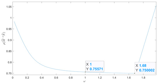
Figure 4. The spectral radius of ${\widehat{M}}^{-1}\widehat{N}$ for $M_i$, $i=7,8$.

We let $A=400I_{1000}+T_{20}\otimes I_{50}+I_{50}\otimes T_{20}$, and $B=380I_{1000}+2I_{50}\otimes T_{20}$, and used the PIM algorithm with $M_9=0.5D-L$, $M_{10}=1.5D-U$, and $t_k=2$, the MPIM algorithm with $M_9=0.5D-L$, $M_{10}=1.5D-U$, $t_k=2$, and $\omega =0.6$, the SOR algorithm with $\omega =0.6$, the M-SSOR algorithm with $\gamma =\omega =0.6$, and the M-SOR algorithm with $\gamma =\omega =0.6$ to solve AVE (1), as shown in Figure 5.

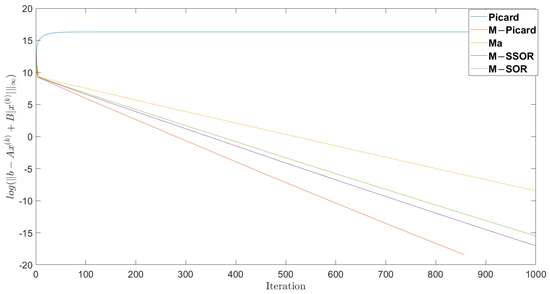
Figure 5. The Rate of Convergency.

The proposed MPIM and Modified SSOR algorithms were significantly better than the methods in the related literature [21,23,24,28].

4. Conclusions

In this paper, we solved AVE (1) by equivalently expressing the implicit fixed-point equation form of the absolute value equations as a two-by-two block nonlinear equation and then proposed an MPIM method for solving it. We also proved the convergence of the MPIM method under suitable choices of the involved parameters and presented the choice of the quasi-optimal parameters. Finally, we performed some numerical experiments to demonstrate that the MPIM method was feasible and effective. However, the convergence analysis and the choice of the optimal parameters of the whole iteration method remain unresolved, which need to be considered in the future.

References

- Rohn, J. A theorem of the alternatives for the equation Ax+B|x|=b. Linear Multilinear Algebra 2004, 52, 421–426. [Google Scholar] [CrossRef]
- Mangasarian, O.L. Absolute value equation solution via concave minimization. Optim. Lett. 2007, 1, 3–8. [Google Scholar] [CrossRef]
- Mangasarian, O.L. A hybrid algorithm for solving the absolute value equation. Optim. Lett. 2015, 9, 1469–1474. [Google Scholar] [CrossRef]
- Mangasarian, O.L.; Meyer, R.R. Absolute value equations. Linear Algebra Appl. 2006, 419, 359–367. [Google Scholar] [CrossRef]
- Noor, M.A.; Iqbal, J.; Al-Said, E. Residual iterative method for solving absolute value equations. Abstr. Appl. Anal. 2012, 2012, 406232. [Google Scholar] [CrossRef]
- Noor, M.A.; Iqbal, J.; Noor, K.I.; Al-Said, E. On an iterative method for solving absolute value equations. Optim. Lett. 2012, 6, 1027–1033. [Google Scholar] [CrossRef]
- Noor, M.A.; Iqbal, J.; Noor, K.I.; Al-Said, E. Generalized AOR method for solving absolute complementarity problems. J. Appl. Math. 2012, 2012, 743861. [Google Scholar] [CrossRef]
- Ketabchi, S.; Moosaei, H. An efficient method for optimal correcting of absolute value equations by minimal changes in the right hand side. Comput. Math. Appl. 2012, 64, 1882–1885. [Google Scholar] [CrossRef]
- Ketabchi, S.; Moosaei, H. Minimum norm solution to the absolute value equation in the convex case. Optim. Theory Appl. 2012, 154, 1080–1087. [Google Scholar] [CrossRef]
- Ketabchi, S.; Moosaei, H.; Fallhi, S. Optimal error correction of the absolute value equations using a genetic algorithm. Comput. Math. Model. 2013, 57, 2339–2342. [Google Scholar] [CrossRef]
- Moosaei, H.; Ketabchi, S.; Noor, M.A.; Iqbal, J.; Hooshyarbakhsh, V. Some techniques for solving absolute value equations. Appl. Math. Comput. 2015, 268, 696–705. [Google Scholar] [CrossRef]
- Gottle, R.W.; Pang, J.S.; Stone, R.E. The Linear Complementarity Problem; Academic Press: New York, NY, USA, 1992. [Google Scholar]
- Rohn, J. On unique solvability of the absolute value equation. Optim. Lett. 2009, 3, 603–606. [Google Scholar] [CrossRef]
- Wu, S.L.; Guo, P. On the unique solvability of the absolute value equation. J. Optim. Theory Appl. 2016, 169, 705–712. [Google Scholar] [CrossRef]
- Wu, S.L.; Li, C.X. The unique solution of the absolute value equations. Appl. Math. Lett. 2018, 76, 195–200. [Google Scholar] [CrossRef]
- Li, C.X.; Wu, S.L. A note on unique solvability of the absolute value equation. Optim. Lett. 2020, 14, 1957–1960. [Google Scholar]
- Mangasarian, O.L. A generalized Newton method for absolute value equations. Optim. Lett. 2009, 3, 101–108. [Google Scholar] [CrossRef]
- Lian, Y.Y.; Li, C.X.; Wu, S.L. Weaker convergent results of the generalized Newton method for the generalized absolute value equations. Comput. Appl. Math. 2018, 338, 221–226. [Google Scholar] [CrossRef]
- Wang, A.; Cao, Y.; Chen, J.X. Modified Newton-type iteration methods for generalized absolute value equations. Optim. Theory Appl. 2019, 181, 216–230. [Google Scholar] [CrossRef]
- Edalatpour, V.; Hezari, D.; Salkuyeh, D.K. A generalization of the Gauss-Seidel iteration method for solving absolute value equations. Appl. Math. Comput. 2017, 293, 156–167. [Google Scholar] [CrossRef]
- Ke, Y.F.; Ma, C.F. SOR-like iteration method for solving absolute value equations. Appl. Math. Comput. 2017, 311, 195–202. [Google Scholar] [CrossRef]
- Guo, P.; Wu, S.L.; Li, C.X. On the SOR-like iteration method for solving absolute value equations. Appl. Math. Lett. 2019, 97, 107–113. [Google Scholar] [CrossRef]
- Li, C.X.; Wu, S.L. Modified SOR-like iteration method for absolute value equations. Math. Probl. Eng. 2020, 2020, 9231639. [Google Scholar]
- Ali, R.; Ahmad, A.; Ahmad, I.; Ali, A. The modification of the generalized Gauss-Seidel iteration techniques for absolute value equations. Comput. Algor. Numer. Dimen. 2022, 1, 130–136. [Google Scholar]
- Salkuyeh, D.K. The Picard-HSS iteration method for absolute value equations. Optim. Lett. 2014, 8, 2191–2202. [Google Scholar] [CrossRef]
- Zheng, L. The Picard-HSS-SOR iteration method for absolute value equations. J. Inequal. Appl. 2020, 2020, 258. [Google Scholar] [CrossRef]
- Lv, C.Q.; Ma, C.F. Picard splitting method and Picard CG method for solving the absolute value equation. Nonlinear Sci. Appl. 2017, 10, 3643–3654. [Google Scholar] [CrossRef]
- Dehghan, M.; Shirilord, A. Matrix multisplitting Picard-iterative method for solving generalized absolute value matrix equation. Appl. Numer. Math. 2020, 158, 425–438. [Google Scholar] [CrossRef]
- Ali, R.; Khan, I.; Ali, M.A.A. Two new generalized iteration methods for solving absolute value equations using M-matrix. AIMS Math. 2022, 7, 8176. [Google Scholar] [CrossRef]
- Yu, D.; Chen, C.; Yang, Y.; Han, D. An inertial inverse-free dynamical system for solving absolute value equations. J. Ind. Manag. Optim. 2023, 19, 2549–2559. [Google Scholar] [CrossRef]
- Hu, S.L.; Huang, Z.H.; Zhang, Q. A generalized Newton method for absolute value equations associated with second order cones. Comput. Appl. Math. 2011, 235, 1490–1501. [Google Scholar] [CrossRef]
- Iqbal, J.; Arif, M. Symmetric SOR method for absolute complementarity problems. Appl. Math. 2013, 2013, 172060. [Google Scholar] [CrossRef]
- Li, C.X. A modified generalized Newton method for absolute value equations. Optim. Theory Appl. 2016, 170, 1055–1059. [Google Scholar] [CrossRef]
- Wang, H.; Liu, H.; Cao, S. A verification method for enclosing solutions of absolute value equations. Collect. Math. 2013, 64, 17–18. [Google Scholar] [CrossRef]
- Cruz, J.Y.B.; Ferreira, O.P.; Prudente, L.F. On the global convergence of the inexact semi-smooth Newton method for absolute value equation. Comput. Optim. Appl. 2016, 65, 93–108. [Google Scholar] [CrossRef]
Disclaimer/Publisher’s Note: The statements, opinions and data contained in all publications are solely those of the individual author(s) and contributor(s) and not of MDPI and/or the editor(s). MDPI and/or the editor(s) disclaim responsibility for any injury to people or property resulting from any ideas, methods, instructions or products referred to in the content. |
© 2023 by the authors. Licensee MDPI, Basel, Switzerland. This article is an open access article distributed under the terms and conditions of the Creative Commons Attribution (CC BY) license (https://creativecommons.org/licenses/by/4.0/).