An Investigation on Existence, Uniqueness, and Approximate Solutions for Two-Dimensional Nonlinear Fractional Integro-Differential Equations

Abstract

In this research, we provide sufficient conditions to prove the existence of local and global solutions for the general two-dimensional nonlinear fractional integro-differential equations. Furthermore, we prove that these solutions are unique. In addition, we use operational matrices of two-variable shifted Jacobi polynomials via the collocation method to reduce the equations into a system of equations. Error bounds of the presented method are obtained. Five test problems are solved. The obtained numerical results show the accuracy, efficiency, and applicability of the proposed approach.

1. Introduction

In the last decades, many problems, such as acoustic wave problems [1], groundwater pollution and groundwater flow problems [2,3,4,5,6], among others [7,8,9,10], have been shown by using fractional calculus. In addition, many engineering and physical problems, such as problems from control, electrochemistry, rheology, coupling and particle mechanics, viscoelasticity, electromagnetism fluid structure, and porous media (see e.g., [11,12,13,14]), have been mathematically formulated by fractional integro-differential equations (FIDEs). Recently, numerical methods for solving FIDEs have attracted the attention of many researchers. Taheri et al. [15] solved stochastic FIDEs by using the shifted Legendre spectral collocation method. Rahimkhani et al. [16] proposed the Bernoulli pseudo-spectral method for solving nonlinear Volterra FIDEs. Wang et al. [17] developed an approximate scheme based on fractional-order Euler functions to solve weakly singular FIDEs. Babaei et al. [18] considered a sixth-kind Chebyshev collocation method to solve a nonlinear quadratic FIDEs of variable order.

In the presented research, we focus on the following general two-dimensional nonlinear fractional integro-differential Equations (2D-NFIDEs):

$$\begin{array}{cc}\hfill & a{f}_{yy}(x,y)+b{f}_{xx}(x,y)+c{f}_{yx}(x,y)+f(x,y)+\lambda I^{\varrho }f(x,y)=g(x,y)+\Theta (x,y)\hfill \\ \hfill & +\mathsf{\Lambda }(x,y)+\rho (x,y)+\phi (x,y),\hfill \end{array}$$

(1)

with the initial conditions of:

$$\begin{array}{c}\hfill f(x,0)=d_1\left(x\right),f(0,y)=d_2\left(y\right),f_y(x,0)=d_3\left(x\right),f_x(0,y)=d_4\left(y\right),f_x(x,0)=d_5\left(x\right),\end{array}$$

(2)

where $(x,y)\in \mathfrak{D}=[0,{\ell }_1)\times [0,{\ell }_2)$; $\varrho =({\varrho }_1,{\varrho }_2)\in (0,\infty )\times (0,\infty )$; and a, b, c, $\lambda$ are constants, and

$$\begin{array}{cc}\hfill & \Theta (x,y)={\int }_0^x{\int }_0^y{k}_1(x,t,y,s)f^{p_1}(t,s)\mathrm{d}s\mathrm{d}t,\hfill \\ \hfill & \mathsf{\Lambda }(x,y)={\displaystyle \frac{1}{\mathsf{\Gamma }\left({\varrho }_1\right)\mathsf{\Gamma }\left({\varrho }_2\right)}}{\int }_0^x{\int }_0^y{(x-t)}^{{\varrho }_1-1}{(y-s)}^{{\varrho }_2-1}{k}_2(x,t,y,s)f^{p_2}(t,s)\mathrm{d}s\mathrm{d}t,\hfill \\ \hfill & \rho (x,y)={\displaystyle \frac{1}{\mathsf{\Gamma }\left({\varrho }_1\right)\mathsf{\Gamma }\left({\varrho }_2\right)}}{\int }_0^{{\ell }_1}{\int }_0^{{\ell }_2}{({\ell }_1-t)}^{{\varrho }_1-1}{({\ell }_2-s)}^{{\varrho }_2-1}{k}_3(x,t,y,s)f^{p_3}(t,s)\mathrm{d}s\mathrm{d}t,\hfill \\ \hfill & \phi (x,y)={\int }_0^{{\ell }_1}{\int }_0^{{\ell }_2}{k}_4(x,t,y,s)f^{p_4}(t,s)\mathrm{d}s\mathrm{d}t.\hfill \end{array}$$

Here, functions $d_i$(.), $i=1,2,3,4,5$, $k_j(x,t,y,s),j=1,2,3,4$, $g(x,y)$ are known, and $f(x,y)$ is unknown; $I^{\varrho }f(x,y)$ is the left-sided mixed Riemann–Liouville integral of order $\varrho =({\varrho }_1,{\varrho }_2)\in (0,\infty )\times (0,\infty )$ of f denoted by [19]

$$\begin{array}{c}\hfill I^{\varrho }f(x,y)={\displaystyle \frac{1}{\mathsf{\Gamma }\left({\varrho }_1\right)\mathsf{\Gamma }\left({\varrho }_2\right)}}{\int }_0^x{\int }_0^y{(x-t)}^{{\varrho }_1-1}{(y-s)}^{{\varrho }_2-1}f(t,s)\mathrm{d}s\mathrm{d}t;\end{array}$$

and $p_j\ge 1,j=1,2,3,4$ are constants.

While several numerical techniques have been proposed for solving many different problems (see, for instance, [20,21,22,23,24,25,26,27,28,29,30,31,32,33,34,35] and references therein), there were few research studies that developed numerical methods for solving Equations (1) and (2). For example, Najafalizadeh and Ezzati [36] obtained approximate solutions of these equations by using operational matrices of two-dimensional block pulse functions (2D-BPFs) with the order of convergence $O\left(\frac{1}{N}\right)$, $N\in \mathbb{N}$. Maleknejad et al. [37] applied operational matrices based on a hybrid of two-dimensional block-pulse functions and shifted Legendre polynomials (2D-HBPSLs) to solve the general 2D-NFIDEs. The order of convergence of this method was $O(\frac{1}{2^{2M-1}{N}^{M}M!})$.

According to the best of our knowledge, the existence and uniqueness of solutions for Equations (1) and (2) have not been discussed so far. In this research, we provide sufficient conditions to prove that there exist local and global solutions for the general 2D-NFIDEs. Then, we prove that the solutions of these equations are unique. Additionally, we prepare an efficient numerical approach to approximate solutions of the general 2D-NFIDEs with high accuracy.

The rest of this paper is organized as follows: in Section 2, some theorems for the existence and uniqueness of solutions of general 2D-NFIDEs are proved. In Section 3, an introduction of one- and two-variable shifted Jacobi polynomials (1D-SJPs and 2D-SJPs) is provided. Additionally, some operational matrices are introduced. In Section 4, by using the collocation method via these operational matrices, approximate solutions for Equations (1) and (2) are obtained. In Section 5, error bounds of approximations are obtained. In Section 6, five test problems are solved to show the accuracy of the proposed method. In Section 7, a conclusion is presented.

2. Existence and Uniqueness of Solutions

Now, by using Schauder’s fixed-point theorem [38], a local existence of solutions of general 2D-NIDEFs is proved in a Banach space.

Theorem 1.

Suppose that

(C1) 

$0\le t\le x\le {\ell }_1$, $0\le s\le y\le {\ell }_2$, g, $g_1$, f, $v\in C(\mathfrak{D},{\mathbb{R}}^n)$, $k_1$, $k_2$, $k_3$, $k_4\in C(\mathfrak{D}\times \mathfrak{D}\times {\mathbb{R}}^n,{\mathbb{R}}^n)$;

(C2) 

$∥f_{yy}(x,y)-v_{yy}(x,y)∥<\frac{\epsilon }{24a}$, $∥f_{xx}(x,y)-v_{xx}(x,y)∥<\frac{\epsilon }{24b}$, $∥f_{yx}(x,y)-v_{yx}(x,y)∥<\frac{\epsilon }{24c}$, $∥I^{\varrho }f(x,y)-I^{\varrho }v(x,y)∥<\frac{\epsilon }{24\lambda }$;

(C3) 

$∥g(x,y)-g_1(x,y)∥<\frac{\epsilon }{6}$;

(C4) 

$∥k_i(x,t,y,s,f(t,s))-k_i(x,t,y,s,v(t,s))∥<\frac{\epsilon }{6\alpha \beta }$, $i=1,4$, $0<\alpha <{\ell }_1$, $0<\beta <{\ell }_2$;

(C5) 

$∥k_j(x,t,y,s,f(t,s))-k_j(x,t,y,s,v(t,s))∥<\frac{\epsilon \mathsf{\Gamma }({\varrho }_1+1)\mathsf{\Gamma }({\varrho }_2+1)}{6{\alpha }^{{\varrho }_1}{\beta }^{{\varrho }_2}}$, $j=2,3$, $0<\alpha <{\ell }_1$, $0<\beta <{\ell }_2$.

Then, there exists at least one solution for the 2D-NIDEF on $0\le t\le \alpha ,0\le s\le \beta$.

Proof. 

Suppose that $\mathcal{D}=\{(x,t,y,s,f):(x,t,y,s)\in \mathfrak{D}\times \mathfrak{D},|f|\le b^{\prime }\}$. Let $\left|f_{yy}(x,y)\right|\le \frac{b^{\prime }}{16a}$, $\left|f_{xx}(x,y)\right|\le \frac{b^{\prime }}{16b}$, $\left|f_{yx}(x,y)\right|\le \frac{b^{\prime }}{16c}$, $\left|I^{\varrho }f(x,y)\right|\le \frac{b^{\prime }}{16\lambda }$, $\left|g(x,y)\right|\le \frac{b^{\prime }}{4}$,

$$max\left\{\right|k_i(x_1,t,y_1,s,f(t,s))|,|k_i(x_2,t,y_2,s,f(t,s))\left|\right\}={\xi }_i,i=1,2,3,4,$$

on $\mathcal{D}$. Choose $({\xi }_1+{\xi }_4)\alpha \beta \le \frac{b^{\prime }}{4}$, $\frac{({\xi }_2+{\xi }_3){\alpha }^{{\varrho }_1}{\beta }^{{\varrho }_2}}{\mathsf{\Gamma }({\varrho }_1+1)\mathsf{\Gamma }({\varrho }_2+1)}\le \frac{b^{\prime }}{4}$. Consider ${\mathsf{\Pi }}_0=\{f:f\in C({\mathfrak{D}}_0,{\mathbb{R}}^n),$$\left|f\right|\le b^{\prime }\}$ such that $∥f∥=\underset{(x,y)\in {\mathfrak{D}}_0}{max}\left|f(x,y)\right|$, ${\mathfrak{D}}_0=[0,\alpha ]\times [0,\beta ]$. Clearly, ${\mathsf{\Pi }}_0$ is bounded, closed, and convex. Now, for any $f\in {\mathsf{\Pi }}_0$, define the operator

$$\begin{array}{cc}\hfill \mathcal{T}f(x,y)=& -a{f}_{yy}(x,y)-b{f}_{xx}(x,y)-c{f}_{yx}(x,y)-\lambda I^{\varrho }f(x,y)+g(x,y)+\Theta (x,y)\hfill \\ \hfill & +\mathsf{\Lambda }(x,y)+\rho (x,y)+\phi (x,y),(x,y)\in {\mathfrak{D}}_0.\hfill \end{array}$$

(3)

It is clear that

$$\begin{array}{cc}\hfill & \left|\Theta (x,y)\right|\le {\xi }_1\alpha \beta ,\hfill \\ \hfill & \left|\mathsf{\Lambda }(x,y)\right|\le \frac{{\xi }_2{\alpha }^{{\varrho }_1}{\beta }^{{\varrho }_2}}{\mathsf{\Gamma }({\varrho }_1+1)\mathsf{\Gamma }({\varrho }_2+1)},\hfill \\ \hfill & \left|\rho (x,y)\right|\le \frac{{\xi }_3{\alpha }^{{\varrho }_1}{\beta }^{{\varrho }_2}}{\mathsf{\Gamma }({\varrho }_1+1)\mathsf{\Gamma }({\varrho }_2+1)},\hfill \\ \hfill & \left|\phi (x,y)\right|\le {\xi }_4\alpha \beta .\hfill \end{array}$$

Therefore, we obtain

$$\begin{array}{cc}\hfill \left|\mathcal{T}f(x,y)\right|& \le \left|a{f}_{yy}(x,y)\right|+\left|b{f}_{xx}(x,y)\right|+\left|c{f}_{yx}(x,y)\right|+\left|\lambda I^{\varrho }f(x,y)\right|+\left|g(x,y)\right|+\left|\Theta (x,y)\right|\hfill \\ \hfill & +\left|\mathsf{\Lambda }(x,y)\right|+\left|\rho (x,y)\right|+\left|\phi (x,y)\right|\hfill \\ \hfill & \le \frac{b^{\prime }}{2}+({\xi }_1+{\xi }_4)\alpha \beta +\frac{({\xi }_2+{\xi }_3){\alpha }^{{\varrho }_1}{\beta }^{{\varrho }_2}}{\mathsf{\Gamma }({\varrho }_1+1)\mathsf{\Gamma }({\varrho }_2+1)}\le b^{\prime },\hfill \end{array}$$

which implies that $\mathcal{T}\left({\mathsf{\Pi }}_0\right)\subset {\mathsf{\Pi }}_0$. Furthermore, for any $(x_1,y_1),(x_2,y_2)\in {\mathfrak{D}}_0$, such that $x_2>x_1$ and $y_2>y_1$, we obtain

$$\begin{array}{cc}\hfill \left|\mathcal{T}f(x_2,y_2)-\mathcal{T}f(x_1,y_1)\right|\le & a\left|f_{yy}(x_2,y_2)-f_{yy}(x_1,y_1)\right|+b\left|f_{xx}(x_2,y_2)-f_{xx}(x_1,y_1)\right|\hfill \\ \hfill & +c\left|f_{yx}(x_2,y_2)-f_{yx}(x_1,y_1)\right|+\lambda \left|I^{\varrho }f(x_2,y_2)-I^{\varrho }f(x_1,y_1)\right|\hfill \\ \hfill & +\left|g(x_2,y_2)-g(x_1,y_1)\right|+\left|\Theta (x_2,y_2)-\Theta (x_1,y_1)\right|\hfill \\ \hfill & +\left|\mathsf{\Lambda }(x_2,y_2)-\mathsf{\Lambda }(x_1,y_1)\right|+\left|\rho (x_2,y_2)-\rho (x_1,y_1)\right|\hfill \\ \hfill & +\left|\phi (x_2,y_2)-\phi (x_1,y_1)\right|.\hfill \end{array}$$

(4)

Additionally, we have

$$\begin{array}{cc}\hfill & \left|I^{\varrho }f(x_2,y_2)-I^{\varrho }f(x_1,y_1)\right|\hfill \\ \hfill & \le \frac{1}{\mathsf{\Gamma }\left({\varrho }_1\right)\mathsf{\Gamma }\left({\varrho }_2\right)}\left|{\int }_0^{x_2}{\int }_0^{y_2}{(x_2-t)}^{{\varrho }_1-1}{(y_2-s)}^{{\varrho }_2-1}f(t,s)\mathrm{d}s\mathrm{d}t\right.\hfill \\ \hfill & \left.-{\int }_0^{x_1}{\int }_0^{y_1}{(x_1-t)}^{{\varrho }_1-1}{(y_1-s)}^{{\varrho }_2-1}f(t,s)\mathrm{d}s\mathrm{d}t\right|\hfill \\ \hfill & \le \frac{1}{\mathsf{\Gamma }\left({\varrho }_1\right)\mathsf{\Gamma }\left({\varrho }_2\right)}\left|{\int }_0^{x_1}{\int }_0^{y_1}{(x_2-t)}^{{\varrho }_1-1}{(y_2-s)}^{{\varrho }_2-1}f(t,s)\mathrm{d}s\mathrm{d}t\right.\hfill \\ \hfill & +{\int }_{x_1}^{x_2}{\int }_{y_1}^{y_2}{(x_2-t)}^{{\varrho }_1-1}{(y_2-s)}^{{\varrho }_2-1}f(t,s)\mathrm{d}s\mathrm{d}t\hfill \\ \hfill & \left.-{\int }_0^{x_1}{\int }_0^{y_1}{(x_1-t)}^{{\varrho }_1-1}{(y_1-s)}^{{\varrho }_2-1}f(t,s)\mathrm{d}s\mathrm{d}t\right|\hfill \\ \hfill & \le \frac{1}{\mathsf{\Gamma }\left({\varrho }_1\right)\mathsf{\Gamma }\left({\varrho }_2\right)}\left|{\int }_0^{x_1}{\int }_0^{y_1}\left({(x_2-t)}^{{\varrho }_1-1}{(y_2-s)}^{{\varrho }_2-1}-{(x_1-t)}^{{\varrho }_1-1}{(y_1-s)}^{{\varrho }_2-1}\right)f(t,s)\mathrm{d}s\mathrm{d}t\right.\hfill \\ \hfill & \left.+{\int }_{x_1}^{x_2}{\int }_{y_1}^{y_2}{(x_2-t)}^{{\varrho }_1-1}{(y_2-s)}^{{\varrho }_2-1}f(t,s)\mathrm{d}s\mathrm{d}t\right|\hfill \\ \hfill & \le \frac{b^{\prime }}{\mathsf{\Gamma }({\varrho }_1+1)\mathsf{\Gamma }({\varrho }_2+1)}\left({\int }_0^{x_1}{\int }_0^{y_1}\left({(x_2-t)}^{{\varrho }_1-1}{(y_2-s)}^{{\varrho }_2-1}-{(x_1-t)}^{{\varrho }_1-1}{(y_1-s)}^{{\varrho }_2-1}\right)\mathrm{d}s\mathrm{d}t\right.\hfill \\ \hfill & \left.+{\int }_{x_1}^{x_2}{\int }_{y_1}^{y_2}{(x_2-t)}^{{\varrho }_1-1}{(y_2-s)}^{{\varrho }_2-1}\mathrm{d}s\mathrm{d}t\right)\hfill \\ \hfill & \le \frac{b^{\prime }}{\mathsf{\Gamma }({\varrho }_1+1)\mathsf{\Gamma }({\varrho }_2+1)}\left({(x_2-x_1)}^{{\varrho }_1}{(y_2-y_1)}^{{\varrho }_2}-x_2^{{\varrho }_1}{y}_2^{{\varrho }_2}+x_1^{{\varrho }_1}{y}_1^{{\varrho }_2}-{(x_2-x_1)}^{{\varrho }_1}{(y_2-y_1)}^{{\varrho }_2}\right)\hfill \\ \hfill & =0.\hfill \end{array}$$

Therefore,

$$\begin{array}{c}\hfill \left|\mathcal{T}f(x_2,y_2)-\mathcal{T}f(x_1,y_1)\right|=0.\end{array}$$

(5)

Moreover, we can obtain

$$\begin{array}{cc}\hfill & \left|\mathsf{\Lambda }(x_2,y_2)-\mathsf{\Lambda }(x_1,y_1)\right|\le \frac{1}{\mathsf{\Gamma }\left({\varrho }_1\right)\mathsf{\Gamma }\left({\varrho }_2\right)}\left|{\int }_0^{x_2}{\int }_0^{y_2}{(x_2-t)}^{{\varrho }_1-1}{(y_2-s)}^{{\varrho }_2-1}{k}_2(x_2,t,y_2,s,f(t,s))\mathrm{d}s\mathrm{d}t\right.\hfill \\ \hfill & \left.-{\int }_0^{x_1}{\int }_0^{y_1}{(x_1-t)}^{{\varrho }_1-1}{(y_1-s)}^{{\varrho }_2-1}{k}_2(x_1,t,y_1,s,f(t,s))\mathrm{d}s\mathrm{d}t\right|\hfill \\ \hfill & =\frac{1}{\mathsf{\Gamma }\left({\varrho }_1\right)\mathsf{\Gamma }\left({\varrho }_2\right)}\left|{\int }_0^{x_1}{\int }_0^{y_1}{(x_2-t)}^{{\varrho }_1-1}{(y_2-s)}^{{\varrho }_2-1}{k}_2(x_2,t,y_2,s,f(t,s))\mathrm{d}s\mathrm{d}t\right.\hfill \\ \hfill & +{\int }_{x_1}^{x_2}{\int }_{y_1}^{y_2}{(x_2-t)}^{{\varrho }_1-1}{(y_2-s)}^{{\varrho }_2-1}{k}_2(x_2,t,y_2,s,f(t,s))\mathrm{d}s\mathrm{d}t\hfill \\ \hfill & \left.-{\int }_0^{x_1}{\int }_0^{y_1}{(x_1-t)}^{{\varrho }_1-1}{(y_1-s)}^{{\varrho }_2-1}{k}_2(x_1,t,y_1,s,f(t,s))\mathrm{d}s\mathrm{d}t\right|\hfill \\ \hfill & =\frac{1}{\mathsf{\Gamma }\left({\varrho }_1\right)\mathsf{\Gamma }\left({\varrho }_2\right)}\left|{\int }_0^{x_1}{\int }_0^{y_1}\left({(x_2-t)}^{{\varrho }_1-1}{(y_2-s)}^{{\varrho }_2-1}{k}_2(x_2,t,y_2,s,f(t,s))\right.\right.\hfill \\ \hfill & \left.-{(x_1-t)}^{{\varrho }_1-1}{(y_1-s)}^{{\varrho }_2-1}{k}_2(x_1,t,y_1,s,f(t,s))\right)\mathrm{d}s\mathrm{d}t\hfill \\ \hfill & \left.+{\int }_{x_1}^{x_2}{\int }_{y_1}^{y_2}{(x_2-t)}^{{\varrho }_1-1}{(y_2-s)}^{{\varrho }_2-1}{k}_2(x_2,t,y_2,s,f(t,s))\mathrm{d}s\mathrm{d}t\right|\hfill \\ \hfill & \le \frac{1}{\mathsf{\Gamma }\left({\varrho }_1\right)\mathsf{\Gamma }\left({\varrho }_2\right)}{\int }_0^{x_1}{\int }_0^{y_1}\left({(x_2-t)}^{{\varrho }_1-1}{(y_2-s)}^{{\varrho }_2-1}\left|k_2(x_2,t,y_2,s,f(t,s))\right|\right.\hfill \\ \hfill & \left.+{(x_1-t)}^{{\varrho }_1-1}{(y_1-s)}^{{\varrho }_2-1}\left|k_2(x_1,t,y_1,s,f(t,s))\right|\right)\mathrm{d}s\mathrm{d}t\hfill \\ \hfill & +\frac{1}{\mathsf{\Gamma }\left({\varrho }_1\right)\mathsf{\Gamma }\left({\varrho }_2\right)}{\int }_{x_1}^{x_2}{\int }_{y_1}^{y_2}{(x_2-t)}^{{\varrho }_1-1}{(y_2-s)}^{{\varrho }_2-1}\left|k_2(x_2,t,y_2,s,f(t,s))\right|\mathrm{d}s\mathrm{d}t\hfill \\ \hfill & \le \frac{{\xi }_2}{\mathsf{\Gamma }\left({\varrho }_1\right)\mathsf{\Gamma }\left({\varrho }_2\right)}\left({\int }_0^{x_1}{\int }_0^{y_1}\left({(x_2-t)}^{{\varrho }_1-1}{(y_2-s)}^{{\varrho }_2-1}+{(x_1-t)}^{{\varrho }_1-1}{(y_1-s)}^{{\varrho }_2-1}\right)\mathrm{d}s\mathrm{d}t\right.\hfill \\ \hfill & \left.+{\int }_{x_1}^{x_2}{\int }_{y_1}^{y_2}{(x_2-t)}^{{\varrho }_1-1}{(y_2-s)}^{{\varrho }_2-1}\mathrm{d}s\mathrm{d}t\right)\hfill \\ \hfill & \le \frac{{\xi }_2}{\mathsf{\Gamma }({\varrho }_1+1)\mathsf{\Gamma }({\varrho }_2+1)}\left({(x_2-x_1)}^{{\varrho }_1}{(y_2-y_1)}^{{\varrho }_2}-x_2^{{\varrho }_1}{y}_2^{{\varrho }_2}+x_1^{{\varrho }_1}{y}_1^{{\varrho }_2}+{(x_2-x_1)}^{{\varrho }_1}{(y_2-y_1)}^{{\varrho }_2}\right)\hfill \\ \hfill & \le \frac{2{\xi }_2}{\mathsf{\Gamma }({\varrho }_1+1)\mathsf{\Gamma }({\varrho }_2+1)}{(x_2-x_1)}^{{\varrho }_1}{(y_2-y_1)}^{{\varrho }_2}.\hfill \end{array}$$

(6)

Similarly,

$$\begin{array}{cc}\hfill & \left|\Theta (x_2,y_2)-\Theta (x_1,y_1)\right|\le {\xi }_1(x_2{y}_2-x_1{y}_1),\hfill \end{array}$$

(7)

$$\begin{array}{cc}\hfill & \left|\rho (x_2,y_2)-\rho (x_1,y_1)\right|\le {\xi }_3\left(\frac{{\alpha }^{{\varrho }_1}{\beta }^{{\varrho }_2}}{\mathsf{\Gamma }({\varrho }_1+1)\mathsf{\Gamma }({\varrho }_2+1)}-\frac{{\alpha }^{{\varrho }_1}{\beta }^{{\varrho }_2}}{\mathsf{\Gamma }({\varrho }_1+1)\mathsf{\Gamma }({\varrho }_2+1)}\right)=0,\hfill \end{array}$$

(8)

$$\begin{array}{cc}\hfill & \left|\phi (x_2,y_2)-\phi (x_1,y_1)\right|\le {\xi }_4(\alpha \beta -\alpha \beta )=0.\hfill \end{array}$$

(9)

Applying inequalities (5)–(9) in (4) gives

$$\begin{array}{cc}\hfill \left|\mathcal{T}f(x_2,y_2)-\mathcal{T}f(x_1,y_1)\right|\le & \left|\left(\mathcal{F}f\right)(x_2,y_2)-\left(\mathcal{F}f\right)(x_1,y_1)\right|+\lambda \left|I^{\varrho }f(x_2,y_2)-I^{\varrho }f(x_1,y_1)\right|\hfill \\ \hfill & +\left|g(x_2,y_2)-g(x_1,y_1)\right|+{\xi }_1(x_2{y}_2-x_1{y}_1)\hfill \\ \hfill & +\frac{2{\xi }_2}{\mathsf{\Gamma }({\varrho }_1+1)\mathsf{\Gamma }({\varrho }_2+1)}{(x_2-x_1)}^{{\varrho }_1}{(y_2-y_1)}^{{\varrho }_2},\hfill \end{array}$$

(10)

where

$$\begin{array}{c}\hfill \left(\mathcal{F}f\right)(x,y)=-a{f}_{yy}(x,y)-b{f}_{xx}(x,y)-c{f}_{yx}(x,y).\end{array}$$

It is clear that the right-hand side of (10) tends to zero as $x_2\to x_1,y_2\to y_1$. Thus, $\mathcal{T}:{\mathsf{\Pi }}_0\to {\mathsf{\Pi }}_0$ is equicontinuous. Therefore, by using the Arzela–Ascoli theorem [39], the compactness of the closure of $\mathcal{T}\left({\mathsf{\Pi }}_0\right)$ can be concluded.

Now, we need to show that $\mathcal{T}$ is continuous. For this propose, define

$$\mathcal{T}v(x,y)=\left(\mathcal{F}v\right)(x,y)-\lambda I^{\varrho }v(x,y)+g_1(x,y)+{\Theta }_v(x,y)+{\mathsf{\Lambda }}_v(x,y)+{\rho }_v(x,y)+{\phi }_v(x,y),$$

$$v(x,0)=d_1\left(x\right),v(0,y)=d_2\left(y\right),v_y(x,0)=d_3\left(x\right),v_x(0,y)=d_4\left(y\right),v_x(x,0)=d_5\left(x\right),$$

where $(x,y)\in {\mathfrak{D}}_0$, $v\in {\mathsf{\Pi }}_0$, and

$$\begin{array}{cc}\hfill & \left(\mathcal{F}v\right)(x,y)=-a{v}_{yy}(x,y)-b{v}_{xx}(x,y)-c{v}_{yx}(x,y),\hfill \\ \hfill & {\Theta }_v(x,y)={\int }_0^x{\int }_0^y{k}_1(x,t,y,s,v(t,s))\mathrm{d}s\mathrm{d}t,\hfill \\ \hfill & {\mathsf{\Lambda }}_v(x,y)={\displaystyle \frac{1}{\mathsf{\Gamma }\left({\varrho }_1\right)\mathsf{\Gamma }\left({\varrho }_2\right)}}{\int }_0^x{\int }_0^y{(x-t)}^{{\varrho }_1-1}{(y-s)}^{{\varrho }_2-1}{k}_2(x,t,y,s,v(t,s))\mathrm{d}s\mathrm{d}t,\hfill \\ \hfill & {\rho }_v(x,y)={\displaystyle \frac{1}{\mathsf{\Gamma }\left({\varrho }_1\right)\mathsf{\Gamma }\left({\varrho }_2\right)}}{\int }_0^{\alpha }{\int }_0^{\beta }{(\alpha -t)}^{{\varrho }_1-1}{(\beta -s)}^{{\varrho }_2-1}{k}_3(x,t,y,s,v(t,s))\mathrm{d}s\mathrm{d}t,\hfill \\ \hfill & {\phi }_v(x,y)={\int }_0^{\alpha }{\int }_0^{\beta }{k}_4(x,t,y,s,v(t,s))\mathrm{d}s\mathrm{d}t.\hfill \end{array}$$

Since $k_i,i=1,2,3,4,$ are uniformly continuous, we can write

$$\begin{array}{c}\hfill \forall \epsilon >0,\exists \delta >0:\left|f\right(x,y)-v(x,y\left)\right|<\delta .\end{array}$$

Suppose that the assumptions $\left(\mathbf{C}\mathbf{1}\right)$–$\left(\mathbf{C}\mathbf{5}\right)$ hold; therefore,

$$\begin{array}{cc}\hfill \left|\mathcal{T}f(x,y)-\mathcal{T}v(x,y)\right|\le & \left|\left(\mathcal{F}f\right)(x,y)-\left(\mathcal{F}v\right)(x,y)\right|+\lambda \left|I^{\varrho }f(x,y)-I^{\varrho }v(x,y)\right|\hfill \\ \hfill & +\left|g(x,y)-g_1(x,y)\right|+\left|\Theta (x,y)-{\Theta }_v(x,y)\right|\hfill \\ \hfill & +\left|\mathsf{\Lambda }(x,y)-{\mathsf{\Lambda }}_v(x,y)\right|+\left|\rho (x,y)-{\rho }_v(x,y)\right|\hfill \\ \hfill & +\left|\phi (x,y)-{\phi }_v(x,y)\right|.\hfill \end{array}$$

Furthermore, we can easily obtain the following inequalities:

$$\begin{array}{cc}\hfill & \left|\Theta (x,y)-{\Theta }_v(x,y)\right|\le \frac{\epsilon }{6\alpha \beta }{\int }_0^x{\int }_0^y\mathrm{d}s\mathrm{d}t\le \frac{\epsilon }{6},\hfill \\ \hfill & \left|\mathsf{\Lambda }(x,y)-{\mathsf{\Lambda }}_v(x,y)\right|\le \frac{1}{\mathsf{\Gamma }\left({\varrho }_1\right)\mathsf{\Gamma }\left({\varrho }_2\right)}\frac{\epsilon \mathsf{\Gamma }({\varrho }_1+1)\mathsf{\Gamma }({\varrho }_2+1)}{6{\alpha }^{{\varrho }_1}{\beta }^{{\varrho }_2}}{\int }_0^x{\int }_0^y{(x-t)}^{{\varrho }_1-1}{(y-s)}^{{\varrho }_2-1}\mathrm{d}s\mathrm{d}t\le \frac{\epsilon }{6},\hfill \\ \hfill & \left|\rho (x,y)-{\rho }_v(x,y)\right|\le \frac{1}{\mathsf{\Gamma }\left({\varrho }_1\right)\mathsf{\Gamma }\left({\varrho }_2\right)}\frac{\epsilon \mathsf{\Gamma }({\varrho }_1+1)\mathsf{\Gamma }({\varrho }_2+1)}{6{\alpha }^{{\varrho }_1}{\beta }^{{\varrho }_2}}{\int }_0^{\alpha }{\int }_0^{\beta }{(\alpha -t)}^{{\varrho }_1-1}{(\beta -s)}^{{\varrho }_2-1}\mathrm{d}s\mathrm{d}t=\frac{\epsilon }{6},\hfill \\ \hfill & \left|\phi (x,y)-{\phi }_v(x,y)\right|\le \frac{\epsilon }{6\alpha \beta }{\int }_0^{\alpha }{\int }_0^{\beta }\mathrm{d}s\mathrm{d}t=\frac{\epsilon }{6}.\hfill \end{array}$$

Thus, we have

$$\begin{array}{c}\hfill \left|\mathcal{T}f(x,y)-\mathcal{T}v(x,y)\right|\le \epsilon ,\end{array}$$

and the proof is completed. □

In the following theorem, by using Tychonoff’s fixed-point theorem [38], the global existence of solutions of the general 2D-NFIDEs will be discussed.

Theorem 2.

Suppose that

(D1) 

$G_i\in C({\mathbb{R}}_{+}^5,{\mathbb{R}}^n)$, $k_i\in C({\mathbb{R}}_{+}^4\times {\mathbb{R}}^n,{\mathbb{R}}^n)$, $i=1,2,3,4$;

(D2) 

For each $(x,t,y,s)\in {\mathbb{R}}_{+}^4$, $G_i(x,t,y,s,u(t,s))$, $i=1,2,3,4,$ are monotonically non-decreasing in u;

(D3) 

$\left|k_i(x,t,y,s,f(t,s))\right|\le G_i(x,t,y,s,\left|f(t,s)\right|)$, $(x,t,y,s,f(t,s))\in {\mathbb{R}}_{+}^4\times {\mathbb{R}}^n$, $i=1,2,3,4$;

(D4) 

$\left|\left(\mathcal{F}f\right)(x,y)\right|\le \left(\mathcal{F}u\right)(x,y)$.

Then, for every $x,y\ge 0$, the generalized two-dimensional nonlinear fractional integro-differential equation

$$\begin{array}{c}\hfill u(x,y)=\left(\mathcal{F}u\right)(x,y)+{\lambda }^{\prime }{I}^{\varrho }u(x,y)+q(x,y)+{\Theta }_u(x,y)+{\mathsf{\Lambda }}_u(x,y)+{\rho }_u(x,y)+{\phi }_u(x,y),\end{array}$$

(11)

has a solution $u(x,y)$ with initial conditions

$$\begin{array}{c}\hfill u(x,0)=d_1\left(x\right),u(0,y)=d_2\left(y\right),u_y(x,0)=d_3\left(x\right),u_x(0,y)=d_4\left(y\right),u_x(x,0)=d_5\left(x\right),\end{array}$$

(12)

and

$$\begin{array}{cc}\hfill & \left(\mathcal{F}u\right)(x,y)=-a{u}_{yy}(x,y)-b{u}_{xx}(x,y)-c{u}_{yx}(x,y),\hfill \\ \hfill & I^{\varrho }u(x,y)={\displaystyle \frac{1}{\mathsf{\Gamma }\left({\varrho }_1\right)\mathsf{\Gamma }\left({\varrho }_2\right)}}{\int }_0^x{\int }_0^y{(x-t)}^{{\varrho }_1-1}{(y-s)}^{{\varrho }_2-1}u(t,s)\mathrm{d}s\mathrm{d}t,\hfill \\ \hfill & {\Theta }_u(x,y)={\int }_0^x{\int }_0^y{G}_1(x,t,y,s,u(t,s))\mathrm{d}s\mathrm{d}t,\hfill \\ \hfill & {\mathsf{\Lambda }}_u(x,y)={\displaystyle \frac{1}{\mathsf{\Gamma }\left({\varrho }_1\right)\mathsf{\Gamma }\left({\varrho }_2\right)}}{\int }_0^x{\int }_0^y{(x-t)}^{{\varrho }_1-1}{(y-s)}^{{\varrho }_2-1}{G}_2(x,t,y,s,u(t,s))\mathrm{d}s\mathrm{d}t,\hfill \\ \hfill & {\rho }_u(x,y)={\displaystyle \frac{1}{\mathsf{\Gamma }\left({\varrho }_1\right)\mathsf{\Gamma }\left({\varrho }_2\right)}}{\int }_0^{{\ell }_1}{\int }_0^{{\ell }_2}{({\ell }_1-t)}^{{\varrho }_1-1}{({\ell }_2-s)}^{{\varrho }_2-1}{G}_3(x,t,y,s,u(t,s))\mathrm{d}s\mathrm{d}t,\hfill \\ \hfill & {\phi }_u(x,y)={\int }_0^{{\ell }_1}{\int }_0^{{\ell }_2}{G}_4(x,t,y,s,u(t,s))\mathrm{d}s\mathrm{d}t.\hfill \end{array}$$

Additionally, for every $x,y\ge 0$ and $q(x,y)\in {\mathbb{R}}_{+}^2$, such that $\left|g(x,y)\right|\le q(x,y)$, there exists a solution $f(x,y)$ for Equations (1) and (2) satisfying $\left|f(x,y)\right|\le u(x,y)$ and $\left|\lambda \right|\le {\lambda }^{\prime }$.

Proof. 

Let $\mathcal{Q}$ be a real space of all continuous functions from $(0,\infty )\times (0,\infty )$ into ${\mathbb{R}}^n$. The topology on $\mathcal{Q}$ is that induced by the family of pseudo-norms ${\left\{{\mathcal{Q}}_{m^{\prime },m}\left(f\right)\right\}}_{m^{\prime },m=1}^{\infty }$, where ${\mathcal{Q}}_{m^{\prime },m}\left(f\right)=\underset{0\le x\le m^{\prime },0\le y\le m}{sup}\left|f(x,y)\right|$ for $f\in \mathcal{Q}$. Consider ${\left\{{\mathcal{S}}_{m^{\prime },m}\right\}}_{m^{\prime },m=1}^{\infty }$ as a set of neighborhoods with ${\mathcal{S}}_{m^{\prime },m}=\{f\in \mathcal{Q}:{\mathcal{Q}}_{m^{\prime },m}\left(f\right)\le 1\}$. Under this topology, $\mathcal{Q}$ is complete, locally convex, and a linear space.

Let

$$\begin{array}{c}\hfill {\mathcal{Q}}_0=\{f\in \mathcal{Q}:\left|f(x,y)\right|\le u(x,y),x,y\ge 0\}\subseteq \mathcal{Q},\end{array}$$

where $u(x,y)$ is a solution of Equations (11) and (12). Obviously, in the topology of $\mathcal{Q}$, ${\mathcal{Q}}_0$ is closed, convex, and bounded.

Note that a fixed point of Equations (11) and (12) corresponds to a solution of Equations (1) and (2). Since, in the topology of $\mathcal{Q}$, $\mathcal{T}$ is compact and ${\mathcal{Q}}_0$ is bounded, therefore, the closure of $T\left({\mathcal{Q}}_0\right)$ is compact.

Considering assumptions $\left(\mathbf{D}\mathbf{1}\right)$–$\left(\mathbf{D}\mathbf{4}\right)$ yields

$$\begin{array}{cc}\hfill \left|\Theta (x,y)\right|& \le {\int }_0^x{\int }_0^y\left|k_1(x,t,y,s,f(t,s))\right|\mathrm{d}s\mathrm{d}t\le {\int }_0^x{\int }_0^y{G}_1(x,t,y,s,\left|f(t,s)\right|)\mathrm{d}s\mathrm{d}t\hfill \\ \hfill & \le {\int }_0^x{\int }_0^y{G}_1(x,t,y,s,u(t,s))\mathrm{d}s\mathrm{d}t={\Theta }_u(x,y).\hfill \end{array}$$

Similarly,

$$\begin{array}{c}\hfill \left|\mathsf{\Lambda }(x,y)\right|\le {\mathsf{\Lambda }}_u(x,y),\left|\rho (x,y)\right|\le {\rho }_u(x,y),\left|\phi (x,y)\right|\le {\phi }_u(x,y),\left|I^{\varrho }f(x,y)\right|\le u(x,y).\end{array}$$

Since $u(x,y)$ is a solution of Equations (11) and (12), the definition of ${\mathcal{Q}}_0$ yields $\left|\mathcal{T}f(x,y)\right|\le u(x,y)$. Therefore, $\mathcal{T}\left({\mathcal{Q}}_0\right)\subset {\mathcal{Q}}_0$. Now, by using Tychonoff’s fixed-point theorem [38], we can deduce that $\mathcal{T}$ has a fixed point in ${\mathcal{Q}}_0$, and this completes the proof. □

In the following theorem, we prove that the general 2D-NFIDE has a unique solution.

Theorem 3.

Consider $k_i\in C(\mathfrak{D}\times \mathfrak{D}\times {\mathbb{R}}^n,{\mathbb{R}}^n)$ ($i=1,2,3,4$), $f\in C(\mathfrak{D},{\mathbb{R}}^n)$. Assume that there exist $0<L_j<1$$(j=1,2,3)$ such that:

$$\begin{array}{cc}\hfill & \left|f_{yy}(x,y)-{\overline{f}}_{yy}(x,y)\right|\le L_1\left|f(x,y)-\overline{f}(x,y)\right|,\hfill \end{array}$$

(13)

$$\begin{array}{cc}\hfill & \left|f_{xx}(x,y)-{\overline{f}}_{xx}(x,y)\right|\le L_2\left|f(x,y)-\overline{f}(x,y)\right|,\hfill \end{array}$$

(14)

$$\begin{array}{cc}\hfill & \left|f_{yx}(x,y)-{\overline{f}}_{yx}(x,y)\right|\le L_3\left|f(x,y)-\overline{f}(x,y)\right|,\hfill \end{array}$$

(15)

$$\begin{array}{cc}\hfill & \left|k_i(x,t,y,s,f(t,s))-k_i(x,t,y,s,\overline{f}(t,s))\right|\le {\eta }_i\left|f(t,s)-\overline{f}(t,s)\right|,i=1,2,3,4.\hfill \end{array}$$

(16)

If

$$\begin{array}{c}\hfill \left((a{L}_1+b{L}_2+c{L}_3)+\frac{{\ell }_1^{{\varrho }_1}{\ell }_2^{{\varrho }_2}}{\mathsf{\Gamma }({\varrho }_1+1)\mathsf{\Gamma }({\varrho }_2+1)}\left(\lambda +{\eta }_1+{\eta }_2+{\eta }_3+{\eta }_4\right)\right)<1,\end{array}$$

(17)

then the general 2D-NIDEF has a unique solution.

Proof. 

Let

$$\begin{array}{c}\hfill \mathcal{T}\overline{f}(x,y)=\left(\mathcal{F}\overline{f}\right)(x,y)-\lambda I^{\varrho }\overline{f}(x,y)+g(x,y)+\overline{\Theta }(x,y)+\overline{\mathsf{\Lambda }}(x,y)+\overline{\rho }(x,y)+\overline{\phi }(x,y),\end{array}$$

with

$$\begin{array}{c}\hfill \overline{f}(x,0)=d_1\left(x\right),\overline{f}(0,y)=d_2\left(y\right),{\overline{f}}_y(x,0)=d_3\left(x\right),{\overline{f}}_x(0,y)=d_4\left(y\right),{\overline{f}}_x(x,0)=d_5\left(x\right),\end{array}$$

and

$$\begin{array}{cc}\hfill & \left(\mathcal{F}\overline{f}\right)(x,y)=-a{\overline{f}}_{yy}(x,y)-b{\overline{f}}_{xx}(x,y)-c{\overline{f}}_{yx}(x,y),\hfill \\ \hfill & \overline{\Theta }(x,y)={\int }_0^x{\int }_0^y{k}_1(x,t,y,s){\overline{f}}^{p_1}(t,s)\mathrm{d}s\mathrm{d}t,\hfill \\ \hfill & \overline{\mathsf{\Lambda }}(x,y)={\displaystyle \frac{1}{\mathsf{\Gamma }\left({\varrho }_1\right)\mathsf{\Gamma }\left({\varrho }_2\right)}}{\int }_0^x{\int }_0^y{(x-t)}^{{\varrho }_1-1}{(y-s)}^{{\varrho }_2-1}{k}_2(x,t,y,s){\overline{f}}^{p_2}(t,s)\mathrm{d}s\mathrm{d}t,\hfill \\ \hfill & \overline{\rho }(x,y)={\displaystyle \frac{1}{\mathsf{\Gamma }\left({\varrho }_1\right)\mathsf{\Gamma }\left({\varrho }_2\right)}}{\int }_0^{{\ell }_1}{\int }_0^{{\ell }_2}{({\ell }_1-t)}^{{\varrho }_1-1}{({\ell }_2-s)}^{{\varrho }_2-1}{k}_3(x,t,y,s){\overline{f}}^{p_3}(t,s)\mathrm{d}s\mathrm{d}t,\hfill \\ \hfill & \overline{\phi }(x,y)={\int }_0^{{\ell }_1}{\int }_0^{{\ell }_2}{k}_4(x,t,y,s){\overline{f}}^{p_4}(t,s)\mathrm{d}s\mathrm{d}t.\hfill \end{array}$$

for $(x,y)\in \mathfrak{D}$.

Using (13)–(16) yields

$$\begin{array}{cc}\hfill & \left|\left(\mathcal{F}f\right)(x,y)-\left(\mathcal{F}\overline{f}\right)(x,y)\right|\le (a{L}_1+b{L}_2+c{L}_3)∥f-\overline{f}∥,\hfill \\ \hfill & \left|I^{\varrho }f(x,y)-\lambda I^{\varrho }\overline{f}(x,y)\right|\le \frac{{\ell }_1^{{\varrho }_1}{\ell }_2^{{\varrho }_2}}{\mathsf{\Gamma }({\varrho }_1+1)\mathsf{\Gamma }({\varrho }_2+1)}∥f-\overline{f}∥,\hfill \\ \hfill & \left|\Theta (x,y)-\overline{\Theta }(x,y)\right|\le \frac{{\eta }_1{\ell }_1^{{\varrho }_1}{\ell }_2^{{\varrho }_2}}{\mathsf{\Gamma }({\varrho }_1+1)\mathsf{\Gamma }({\varrho }_2+1)}∥f-\overline{f}∥,\hfill \\ \hfill & \left|\mathsf{\Lambda }(x,y)-\overline{\mathsf{\Lambda }}(x,y)\right|\le \frac{{\eta }_2{\ell }_1^{{\varrho }_1}{\ell }_2^{{\varrho }_2}}{\mathsf{\Gamma }({\varrho }_1+1)\mathsf{\Gamma }({\varrho }_2+1)}∥f-\overline{f}∥,\hfill \\ \hfill & \left|\rho (x,y)-\overline{\rho }(x,y)\right|\le \frac{{\eta }_3{\ell }_1^{{\varrho }_1}{\ell }_2^{{\varrho }_2}}{\mathsf{\Gamma }({\varrho }_1+1)\mathsf{\Gamma }({\varrho }_2+1)}∥f-\overline{f}∥,\hfill \\ \hfill & \left|\phi (x,y)-\overline{\phi }(x,y)\right|\le \frac{{\eta }_4{\ell }_1^{{\varrho }_1}{\ell }_2^{{\varrho }_2}}{\mathsf{\Gamma }({\varrho }_1+1)\mathsf{\Gamma }({\varrho }_2+1)}∥f-\overline{f}∥.\hfill \end{array}$$

Now, we can write

$$\begin{array}{cc}\hfill \left|\mathcal{T}f(x,y)-\mathcal{T}\overline{f}(x,y)\right|\le & \left|\left(\mathcal{F}f\right)(x,y)-\left(\mathcal{F}\overline{f}\right)(x,y)\right|+\lambda \left|I^{\varrho }f(x,y)-\lambda I^{\varrho }\overline{f}(x,y)\right|\hfill \\ \hfill & +\left|\Theta (x,y)-\overline{\Theta }(x,y)\right|+\left|\mathsf{\Lambda }(x,y)-\overline{\mathsf{\Lambda }}(x,y)\right|\hfill \\ \hfill & +\left|\rho (x,y)-\overline{\rho }(x,y)\right|+\left|\phi (x,y)-\overline{\phi }(x,y)\right|\hfill \\ \hfill \le & \left(a{L}_1+b{L}_2+c{L}_3+\frac{{\ell }_1^{{\varrho }_1}{\ell }_2^{{\varrho }_2}}{\mathsf{\Gamma }({\varrho }_1+1)\mathsf{\Gamma }({\varrho }_2+1)}\left(\lambda +{\eta }_1+{\eta }_2+{\eta }_3+{\eta }_4\right)\right)∥f-\overline{f}∥,\hfill \end{array}$$

for any $(x,y)\in \mathfrak{D}$ and $f,\overline{f}\in C(\mathfrak{D},{\mathbb{R}}^n)$. Therefore,

$$\begin{array}{c}\hfill ∥\mathcal{T}f-\mathcal{T}\overline{f}∥\le \left(a{L}_1+b{L}_2+c{L}_3+\frac{{\ell }_1^{{\varrho }_1}{\ell }_2^{{\varrho }_2}}{\mathsf{\Gamma }({\varrho }_1+1)\mathsf{\Gamma }({\varrho }_2+1)}\left(\lambda +{\eta }_1+{\eta }_2+{\eta }_3+{\eta }_4\right)\right)∥f-\overline{f}∥.\end{array}$$

From (17), $\mathcal{T}$ is a contraction map in $C(\mathfrak{D},{\mathbb{R}}^n)$, and thus, it has a unique fixed point. Therefore, $f\in C(\mathfrak{D},{\mathbb{R}}^n)$ is a unique solution for the general 2D-NIDEF. □

3. The 1D-SJPs and 2D-SJPs and Their Operational Matrices

3.1. The 1D-SJPs

The 1D-SJPs are defined on the interval $[0,\ell )$ by

$$\begin{array}{c}\hfill {\mathcal{J}}_{\ell ,l}^{(\tau ,\varsigma )}\left(x\right)=\sum _{j=0}^l{(-1)}^{l-j}{\displaystyle \frac{\mathsf{\Gamma }(l+\varsigma +1)\mathsf{\Gamma }(l+j+\tau +\varsigma +1)}{\mathsf{\Gamma }(j+\varsigma +1)\mathsf{\Gamma }(l+\tau +\varsigma +1)(l-j)!j!{\ell }^j}}{x}^j.\end{array}$$

These polynomials are orthogonal on the interval $[0,\ell )$; therefore,

$$\begin{array}{c}\hfill {\int }_0^{{\ell }_1}{\mathcal{J}}_{\ell ,i}^{(\tau ,\varsigma )}\left(x\right){\mathcal{J}}_{\ell ,i^{\prime }}^{(\tau ,\varsigma )}\left(x\right)w_{\ell }^{(\tau ,\varsigma )}\left(x\right)\mathrm{d}x={\delta }_{i{i}^{\prime }}{h}_{\ell ,i}^{(\tau ,\varsigma )},\end{array}$$

where $w_{\ell }^{(\tau ,\varsigma )}\left(x\right)=x^{\varsigma }{(\ell -x)}^{\tau }$ is a weight function, ${\delta }_{i{i}^{\prime }}$ is Kronecker delta, and

$$\begin{array}{c}\hfill h_{\ell ,l}^{(\tau ,\varsigma )}={\displaystyle \frac{{\ell }^{\tau +\varsigma +1}\mathsf{\Gamma }(l+\tau +1)\mathsf{\Gamma }(l+\varsigma +1)}{(2l+\tau +\varsigma +1)l!\mathsf{\Gamma }(l+\tau +\varsigma +1)}}.\end{array}$$

Additionally, these polynomials have the following property:

$$\begin{array}{c}\hfill {\displaystyle \frac{d^i}{d{x}^i}}{\mathcal{J}}_{\ell ,l}^{(\tau ,\varsigma )}\left(x\right)={\displaystyle \frac{\mathsf{\Gamma }(l+\tau +\varsigma +i+1)}{\mathsf{\Gamma }(l+\tau +\varsigma +1)}}{\mathcal{J}}_{\ell ,l-i}^{(\tau +i,\varsigma +i)}\left(x\right).\end{array}$$

(18)

The vector of 1D-SJPs is as follows:

$$\begin{array}{c}\hfill \mathsf{\Psi }\left(x\right)={\left(\begin{array}{cccc}{\mathcal{J}}_{\ell ,0}^{(\tau ,\varsigma )}\left(x\right)& {\mathcal{J}}_{\ell ,1}^{(\tau ,\varsigma )}\left(x\right)& \dots & {\mathcal{J}}_{\ell ,N}^{(\tau ,\varsigma )}\left(x\right)\end{array}\right)}^T.\end{array}$$

(19)

3.2. 2D-SJPs and Function Approximation

The 2D-SJPs are defined on the domain $\mathfrak{D}=[0,{\ell }_1)\times [0,{\ell }_2)$ by

$$\begin{array}{c}\hfill {\mathcal{J}}_{i,j}^{(\tau ,\varsigma )}(x,y)={\mathcal{J}}_{{\ell }_1,i}^{(\tau ,\varsigma )}\left(x\right){\mathcal{J}}_{{\ell }_2,j}^{(\tau ,\varsigma )}\left(y\right),i,j=0,1,\dots ,N.\end{array}$$

These polynomials are orthogonal on $\mathfrak{D}$; therefore,

$$\begin{array}{c}\hfill {\int }_0^{{\ell }_1}{\int }_0^{{\ell }_2}{\mathcal{J}}_{i,j}^{(\tau ,\varsigma )}(x,y){\mathcal{J}}_{i^{\prime },j^{\prime }}^{(\tau ,\varsigma )}(x,y){\omega }^{(\tau ,\varsigma )}(x,y)\mathrm{d}y\mathrm{d}x={\delta }_{i{i}^{\prime }}{\delta }_{j{j}^{\prime }}{h}_{{\ell }_1,i}^{(\tau ,\varsigma )}{h}_{{\ell }_2,j}^{(\tau ,\varsigma )},\end{array}$$

where ${\omega }^{(\tau ,\varsigma )}(x,y)=w_{{\ell }_1}^{(\tau ,\varsigma )}\left(x\right)w_{{\ell }_2}^{(\tau ,\varsigma )}\left(y\right)$ is a weight function.

By using 2D-SJPs, we can approximate a continuous function $f(x,y)$ on the domain $\mathfrak{D}=[0,{\ell }_1)\times [0,{\ell }_2)$ as follows:

$$\begin{array}{c}\hfill f(x,y)\simeq f_N(x,y)=\sum _{i=0}^N\sum _{j=0}^N{\widehat{f}}_{ij}{\mathcal{J}}_{i,j}^{(\tau ,\varsigma )}(x,y)={\mathsf{\Psi }}^T(x,y)\widehat{F}={\widehat{F}}^T\mathsf{\Psi }(x,y),\end{array}$$

(20)

where

$$\begin{array}{c}\hfill \widehat{F}={\left(\begin{array}{cccccccccccc}{\widehat{f}}_{00}& {\widehat{f}}_{01}& \dots {\widehat{f}}_{0N}& {\widehat{f}}_{10}& {\widehat{f}}_{11}& \dots & {\widehat{f}}_{1N}& \dots & {\widehat{f}}_{N0}& {\widehat{f}}_{N1}& \dots & {\widehat{f}}_{NN}\end{array}\right)}^T,\end{array}$$

with entries

$$\begin{array}{c}\hfill {\widehat{f}}_{ij}={\displaystyle \frac{1}{h_{{\ell }_1,i}^{(\tau ,\varsigma )}{h}_{{\ell }_2,j}^{(\tau ,\varsigma )}}}{\int }_0^{{\ell }_1}{\int }_0^{{\ell }_2}f(x,y){\mathcal{J}}_{i,j}^{(\tau ,\varsigma )}(x,y){\omega }^{(\tau ,\varsigma )}(x,y)\mathrm{d}y\mathrm{d}x,i,j=0,1,\dots ,N,\end{array}$$

and

$$\begin{array}{cc}\hfill \mathsf{\Psi }(x,y)=& \left({\mathcal{J}}_{0,0}^{(\tau ,\varsigma )}(x,y),\dots {\mathcal{J}}_{0,N}^{(\tau ,\varsigma )}(x,y),{\mathcal{J}}_{1,0}^{(\tau ,\varsigma )}(x,y),\dots {\mathcal{J}}_{1,N}^{(\tau ,\varsigma )}(x,y)\right.\hfill \\ \hfill & {\left.\dots ,{\mathcal{J}}_{N,0}^{(\tau ,\varsigma )}(x,y),\dots {\mathcal{J}}_{N,N}^{(\tau ,\varsigma )}(x,y)\right)}^T,\hfill \end{array}$$

(21)

are ${(N+1)}^2\times 1$ vectors.

Additionally, we can expand a function $k(x,t,y,s)$ on the domain $\mathfrak{D}\times \mathfrak{D}$ with respect to 2D-SJPs as follows:

$$\begin{array}{c}\hfill k(x,t,y,s)\simeq {\mathsf{\Psi }}^T(x,y)K\mathsf{\Psi }(t,s).\end{array}$$

(22)

Here, K is a matrix with entries

$$\begin{array}{c}\hfill K_{i,j}={\displaystyle \frac{{\int }_0^{{\ell }_1}{\int }_0^{{\ell }_2}{\int }_0^{{\ell }_1}{\int }_0^{{\ell }_2}{\mathcal{J}}_{q^{\prime }\left[i\right],q^{″}\left[i\right]}^{(\tau ,\varsigma )}(x,y)k(x,t,y,s){\mathcal{J}}_{q^{\prime }\left[j\right],q^{″}\left[j\right]}^{(\tau ,\varsigma )}(t,s){\omega }^{(\tau ,\varsigma )}(x,y){\omega }^{(\tau ,\varsigma )}(t,s)\mathrm{d}s\mathrm{d}t\mathrm{d}y\mathrm{d}x}{h_{{\ell }_1,q^{\prime }\left[i\right]}^{(\tau ,\varsigma )}{h}_{{\ell }_2,q^{″}\left[i\right]}^{(\tau ,\varsigma )}{h}_{{\ell }_1,q^{\prime }\left[j\right]}^{(\tau ,\varsigma )}{h}_{{\ell }_2,q^{″}\left[j\right]}^{(\tau ,\varsigma )}}},\end{array}$$

where

$$\begin{array}{cc}\hfill & q^{\prime }=[0,\dots ,0,1,\dots ,1,\dots ,N,\dots ,N],\hfill \\ \hfill & q^{″}=[0,\dots ,N,0,\dots ,N,\dots ,0,\dots ,N],\hfill \end{array}$$

and $i,j=1,\dots ,{(N+1)}^2$.

3.3. Operational Matrices of Two-Dimensional Integration

In [40], the authors computed the one-dimensional integration of $\mathsf{\Psi }\left(t\right)$ for $t\in [0,1)$. Similarly, we compute the one-dimensional integration of this vector for $t\in [0,\ell )$, as follows:

$$\begin{array}{c}\hfill {\int }_0^x\mathsf{\Psi }\left(t\right)\mathrm{d}t\simeq {\mathbf{P}}_x\mathsf{\Psi }\left(x\right),\end{array}$$

where ${\mathbf{P}}_x$ is a one-dimensional operational matrix of integration, defined in the following form:

$$\begin{array}{c}\hfill {\mathbf{P}}_x=\left(\begin{array}{cccc}{p}_{{}_{00}}& p_{{}_{01}}& \dots & p_{{}_{0N}}\\ p_{{}_{10}}& p_{{}_{11}}& \dots & p_{{}_{1N}}\\ ⋮& ⋮& \ddots & ⋮\\ p_{{}_{N0}}& p_{{}_{N1}}& \dots & p_{{}_{NN}}\end{array}\right),\end{array}$$

(23)

with the following entries:

$$\begin{array}{c}\hfill p_{{}_{kl}}=\sum _{j=0}^k\left({\displaystyle \frac{{(-1)}^{k-j}\mathsf{\Gamma }(l+\varsigma +1)\mathsf{\Gamma }(k+\varsigma +1)\mathsf{\Gamma }(k+j+\tau +\varsigma +1)\mathsf{\Gamma }(\tau +1)}{h_l\mathsf{\Gamma }(l+\tau +\varsigma +1)\mathsf{\Gamma }(j+\varsigma +1)\mathsf{\Gamma }(k+\tau +\varsigma +1)(j+1)!(k-j)!{\ell }^j}}\right.\\ \hfill \left.\times \sum _{i=0}^l{\displaystyle \frac{{(-1)}^{l-i}\mathsf{\Gamma }(l+i+\tau +\varsigma +1)\mathsf{\Gamma }(i+j+\varsigma +2)\ell }{\mathsf{\Gamma }(i+\varsigma +1)\mathsf{\Gamma }(i+j+\tau +\varsigma +3)i!(l-i)!}}\right),k,l=0,1,\dots ,N.\end{array}$$

Since $\mathsf{\Psi }(x,y)=\mathsf{\Psi }\left(x\right)\otimes \mathsf{\Psi }\left(y\right)$, the two-dimensional integration of $\mathsf{\Psi }(t,s)$ can be obtained as follows:

$$\begin{array}{c}\hfill {\int }_0^x{\int }_0^y\mathsf{\Psi }(t,s)\mathrm{d}s\mathrm{d}t\simeq ({\mathbf{P}}_x\otimes {\mathbf{P}}_y)\mathsf{\Psi }(x,y),x\in [0,{\ell }_1),y\in [0,{\ell }_2),\end{array}$$

(24)

where ⊗ denotes the Kronecker product; ${\mathbf{P}}_x\otimes {\mathbf{P}}_y$ is the ${(N+1)}^2\times {(N+1)}^2$ operational matrix of the two-dimensional integration; and ${\mathbf{P}}_x,{\mathbf{P}}_y$ are $(N+1)\times (N+1)$ one-dimensional operational matrices of integration, defined in Equation (23).

Additionally, it is easy to conclude the following result:

$$\begin{array}{c}\hfill {\int }_0^{{\ell }_1}{\int }_0^{{\ell }_2}\mathsf{\Psi }(t,s)\mathrm{d}s\mathrm{d}t=A_1\otimes A_2,\end{array}$$

(25)

where

$$\begin{array}{c}\hfill A_1={\left(\begin{array}{cccc}{a}_0& a_1& \dots & a_N\end{array}\right)}^T,A_2={\left(\begin{array}{cccc}{a}_0^{\prime }& a_1^{\prime }& \dots & a_N^{\prime }\end{array}\right)}^T,\end{array}$$

with the entries:

$$\begin{array}{cc}\hfill & a_r=\sum _{j=0}^r{(-1)}^{r-j}{\displaystyle \frac{\mathsf{\Gamma }(r+\varsigma +1)\mathsf{\Gamma }(r+j+\tau +\varsigma +1){\ell }_1}{\mathsf{\Gamma }(j+\varsigma +1)\mathsf{\Gamma }(r+\tau +\varsigma +1)(r-j)!(j+1)!}},\hfill \\ \hfill & a_r^{\prime }=\sum _{j=0}^r{(-1)}^{r-j}{\displaystyle \frac{\mathsf{\Gamma }(r+\varsigma +1)\mathsf{\Gamma }(r+j+\tau +\varsigma +1){\ell }_2}{\mathsf{\Gamma }(j+\varsigma +1)\mathsf{\Gamma }(r+\tau +\varsigma +1)(r-j)!(j+1)!}},\hfill \end{array}$$

for $r=0,1,\dots ,N$.

3.4. Operational Matrices of Fractional-Order Integration

In [27], the authors defined an operational matrix of the Riemann–Liouville integral operator of order $\kappa$ by

$$\begin{array}{c}\hfill {\mathbf{I}}^{\ell ,\kappa }=\left(\begin{array}{cccc}{S}_{{}_{00}}& S_{{}_{01}}& \dots & S_{{}_{0N}}\\ S_{{}_{10}}& S_{{}_{11}}& \dots & S_{{}_{1N}}\\ ⋮& ⋮& \ddots & ⋮\\ S_{{}_{N0}}& S_{{}_{N1}}& \dots & S_{{}_{NN}}\end{array}\right),\end{array}$$

with the entries

$$\begin{array}{cc}\hfill & S_{{}_{lr}}=\sum _{m=0}^l\left({\displaystyle \frac{{(-1)}^{l-m}\mathsf{\Gamma }(l+\varsigma +1)\mathsf{\Gamma }(l+m+\tau +\varsigma +1)\mathsf{\Gamma }(m+1)}{\mathsf{\Gamma }(m+\varsigma +1)\mathsf{\Gamma }(l+\tau +\varsigma +1)(l-m)!m!\mathsf{\Gamma }(m+\kappa +1){\ell }^m}}\right.\hfill \\ \hfill & \left.\times \sum _{m^{\prime }=0}^r{\displaystyle \frac{{(-1)}^{r-m^{\prime }}(2r+\tau +\varsigma +1)\mathsf{\Gamma }(r+1)\mathsf{\Gamma }(r+m^{\prime }+\tau +\varsigma +1)\mathsf{\Gamma }(m+\kappa +m^{\prime }+\varsigma +1)\mathsf{\Gamma }(\kappa +1){\ell }^{\kappa }}{\mathsf{\Gamma }(r+\tau +1)\mathsf{\Gamma }(m^{\prime }+\varsigma +1)(r-m^{\prime })!m^{\prime }!\mathsf{\Gamma }(m+\kappa +m^{\prime }+\varsigma +\tau +2)}}\right),\hfill \end{array}$$

for $l,r=0,1,\dots ,N$.

Theorem 4

(see [34]). Let $\varrho =({\varrho }_1,{\varrho }_2)\in (0,\infty )\times (0,\infty )$ and $\mathsf{\Psi }(x,y)$ be the vector of 2D-SJPs. Then

$$\begin{array}{c}\hfill I^{\varrho }\mathsf{\Psi }(x,y)\simeq ({\mathit{I}}^{{\ell }_1,{\varrho }_1}\otimes {\mathit{I}}^{{\ell }_2,{\varrho }_2})\mathsf{\Psi }(x,y),(x,y)\in [0,{\ell }_1)\times [0,{\ell }_2).\end{array}$$

(26)

Here, ${\mathit{I}}^{{\ell }_1,{\varrho }_1}$ and ${\mathit{I}}^{{\ell }_2,{\varrho }_2}$ are operational matrices of a fractional Riemann–Liouville integration of orders ${\varrho }_1$ and ${\varrho }_2$, respectively.

Theorem 5

(see [34]). Let $\kappa >0$. Assume that $\mathsf{\Psi }\left(s\right)$, defined in (19), is the vector of 1D-SJPs. Then,

$$\begin{array}{c}\hfill {\displaystyle \frac{1}{\mathsf{\Gamma }\left(\kappa \right)}}{\int }_0^{\ell }{(\ell -s)}^{\kappa -1}\mathsf{\Psi }\left(s\right)\mathrm{d}s=\mathsf{{\rm Y}},\end{array}$$

(27)

where $\mathsf{{\rm Y}}={\left(\begin{array}{cccc}{\gamma }_{{}_0}& {\gamma }_{{}_1}& \dots & {\gamma }_{{}_N}\end{array}\right)}^T$ and

$$\begin{array}{c}\hfill {\gamma }_{{}_r}=\sum _{j=0}^r{(-1)}^{r-j}{\displaystyle \frac{\mathsf{\Gamma }(r+\varsigma +1)\mathsf{\Gamma }(r+j+\tau +\varsigma +1){\ell }^{\kappa -1}}{\mathsf{\Gamma }(j+\varsigma +1)\mathsf{\Gamma }(r+\tau +\varsigma +1)(r-j)!\mathsf{\Gamma }(j+\kappa +1)}},r=0,1,\dots ,N.\end{array}$$

(28)

Theorem 6

(see [34]). Let ${\varrho }_1,{\varrho }_2>0$. Assume that $\mathsf{\Psi }(t,s)$, defined in (21), is the vector of 2D-SJPs. Then

$$\begin{array}{c}\hfill {\displaystyle \frac{1}{\mathsf{\Gamma }\left({\varrho }_1\right)\mathsf{\Gamma }\left({\varrho }_2\right)}}{\int }_0^{{\ell }_1}{\int }_0^{{\ell }_2}{({\ell }_1-t)}^{{\varrho }_1-1}{({\ell }_2-s)}^{{\varrho }_2-1}\mathsf{\Psi }(t,s)\mathrm{d}s\mathrm{d}t={\mathsf{{\rm Y}}}_1\otimes {\mathsf{{\rm Y}}}_2,\end{array}$$

(29)

where

$$\begin{array}{cc}\hfill & {\mathsf{{\rm Y}}}_1={\left(\begin{array}{cccc}\gamma 1_{{}_0}& \gamma 1_{{}_1}& \dots & \gamma 1_{{}_N}\end{array}\right)}^T,{\mathsf{{\rm Y}}}_2={\left(\begin{array}{cccc}\gamma 2_{{}_0}& \gamma 2_{{}_1}& \dots & \gamma 2_{{}_N}\end{array}\right)}^T,\hfill \end{array}$$

and

$$\begin{array}{cc}\hfill & \gamma 1_{{}_r}=\sum _{j=0}^r{(-1)}^{r-j}{\displaystyle \frac{\mathsf{\Gamma }(r+\varsigma +1)\mathsf{\Gamma }(r+j+\tau +\varsigma +1){\ell }_1^{{\varrho }_1}}{\mathsf{\Gamma }(j+\varsigma +1)\mathsf{\Gamma }(r+\tau +\varsigma +1)(r-j)!\mathsf{\Gamma }(j+{\varrho }_1+1)}},\hfill \\ \hfill & \gamma 2_{{}_r}=\sum _{j=0}^r{(-1)}^{r-j}{\displaystyle \frac{\mathsf{\Gamma }(r+\varsigma +1)\mathsf{\Gamma }(r+j+\tau +\varsigma +1){\ell }_2^{{\varrho }_2}}{\mathsf{\Gamma }(j+\varsigma +1)\mathsf{\Gamma }(r+\tau +\varsigma +1)(r-j)!\mathsf{\Gamma }(j+{\varrho }_2+1)}},\hfill \end{array}$$

for $r=0,1,\dots ,N$.

3.5. Operational Matrix of Product

Assume that $\mathsf{\Psi }(x,y)$, defined in (21), is the vector of 2D-SJPs. In [34], Rashidinia et al. introduced the operational matrix of the product as follows:

$$\begin{array}{c}\hfill \mathsf{\Psi }(x,y){\mathsf{\Psi }}^T(x,y)\widehat{F}\simeq \tilde{\widehat{F}}\mathsf{\Psi }(x,y),\end{array}$$

(30)

for $(x,y)\in [0,{\ell }_1)\times [0,{\ell }_2)$. Here, $\tilde{\widehat{F}}$ is the operational matrix of the product with the entries

$$\begin{array}{c}\hfill {\tilde{\widehat{F}}}_{m_1(N+1)+n_1+1,m_2(N+1)+n_2+1}={\displaystyle \frac{1}{h_{{\ell }_1,m_2}^{(\tau ,\varsigma )}{h}_{{\ell }_2,n_2}^{(\tau ,\varsigma )}}}\sum _{j=0}^N\sum _{k=0}^N{\widehat{f}}_{jk}{v}_{m_{1}j{m}_2}{v}_{n_{1}k{n}_2},\end{array}$$

where

$$\begin{array}{cc}\hfill & v_{m_{1}j{m}_2}={\int }_0^{{\ell }_1}{\mathcal{J}}_{{\ell }_1,m_1}^{(\tau ,\varsigma )}\left(x\right){\mathcal{J}}_{{\ell }_1,j}^{(\tau ,\varsigma )}\left(x\right){\mathcal{J}}_{{\ell }_1,m_2}^{(\tau ,\varsigma )}\left(x\right)w_{{\ell }_1}^{(\tau ,\varsigma )}\left(x\right)\mathrm{d}x,\hfill \\ \hfill & v_{n_{1}k{n}_2}={\int }_0^{{\ell }_2}{\mathcal{J}}_{{\ell }_2,n_1}^{(\tau ,\varsigma )}\left(y\right){\mathcal{J}}_{{\ell }_2,k}^{(\tau ,\varsigma )}\left(y\right){\mathcal{J}}_{{\ell }_2,n_2}^{(\tau ,\varsigma )}\left(y\right)w_{{\ell }_2}^{(\tau ,\varsigma )}\left(y\right)\mathrm{d}y,\hfill \end{array}$$

for $m_1,n_1,m_2,n_2=0,1,\dots ,N$.

4. Method of Solution

Here, by using the method proposed in Section 3, we solve the general 2D-NFIDEs. First of all, we define

$$\begin{array}{cc}\hfill & f_{yy}(x,y)\simeq f_{yy}^T\mathsf{\Psi }(x,y),\hfill \end{array}$$

(31)

$$\begin{array}{cc}\hfill & f_{xx}(x,y)\simeq f_{xx}^T\mathsf{\Psi }(x,y),\hfill \end{array}$$

(32)

$$\begin{array}{cc}\hfill & f_{yx}(x,y)\simeq f_{yx}^T\mathsf{\Psi }(x,y),\hfill \end{array}$$

(33)

$$\begin{array}{cc}\hfill & g(x,y)\simeq {\mathsf{\Psi }}^T(x,y)G,\hfill \end{array}$$

(34)

$$\begin{array}{cc}\hfill & k_i(x,t,y,s)\simeq {\mathsf{\Psi }}^T(x,y)k_i\mathsf{\Psi }(t,s),i=1,2,3,4,\hfill \end{array}$$

(35)

$$\begin{array}{cc}\hfill & d_1\left(x\right)=f(x,0)\simeq F_{x0}^T\mathsf{\Psi }(x,y),\hfill \end{array}$$

(36)

$$\begin{array}{cc}\hfill & d_2\left(y\right)=f(0,y)\simeq F_{0y}^T\mathsf{\Psi }(x,y),\hfill \end{array}$$

(37)

$$\begin{array}{cc}\hfill & d_3\left(x\right)=f_y(x,0)\simeq F_{yx0}^T\mathsf{\Psi }(x,y),\hfill \end{array}$$

(38)

$$\begin{array}{cc}\hfill & d_4\left(y\right)=f_x(0,y)\simeq F_{x0y}^T\mathsf{\Psi }(x,y),\hfill \end{array}$$

(39)

$$\begin{array}{cc}\hfill & d_5\left(x\right)=f_x(x,0)\simeq F_{xx0}^T\mathsf{\Psi }(x,y).\hfill \end{array}$$

(40)

Now, from the Appendix in [36], we can obtain:

$$\begin{array}{c}\hfill f_{yy}^T=((f^T-F_{x0}^T){(I\otimes {\mathbf{P}}_y)}^{-1}-F_{yx0}^T){(I\otimes {\mathbf{P}}_y)}^{-1},\end{array}$$

(41)

$$\begin{array}{c}\hfill f_{xx}^T=((f^T-F_{0y}^T){({\mathbf{P}}_x\otimes I)}^{-1}-F_{x0y}^T){({\mathbf{P}}_x\otimes I)}^{-1},\end{array}$$

(42)

$$\begin{array}{c}\hfill f_{yx}^T=((f^T-F_{0y}^T){({\mathbf{P}}_x\otimes I)}^{-1}-F_{xx0}^T){(I\otimes {\mathbf{P}}_y)}^{-1}.\end{array}$$

(43)

Using (26) for $I^{\varrho }f(x,y)$ yields

$$\begin{array}{cc}\hfill I^{\varrho }f(x,y)& \simeq I^{\varrho }{\widehat{F}}^T\mathsf{\Psi }(x,y)={\widehat{F}}^T{I}^{\varrho }\mathsf{\Psi }(x,y)={\widehat{F}}^T\left({\mathbf{I}}^{{\ell }_1,{\varrho }_1}\otimes {\mathbf{I}}^{{\ell }_2,{\varrho }_2}\right)\mathsf{\Psi }(x,y).\hfill \end{array}$$

(44)

Additionally, by using (20) and (30), we have

$$\begin{array}{cc}\hfill f^2(x,y)& \simeq {\widehat{F}}^T\mathsf{\Psi }(x,y){\mathsf{\Psi }}^T(x,y)\widehat{F}=\underset{{\widehat{F}}_2}{\underbrace{{\widehat{F}}^T\tilde{\widehat{F}}}}\mathsf{\Psi }(x,y)={\widehat{F}}_2\mathsf{\Psi }(x,y),\hfill \\ \hfill f^3(x,y)& \simeq {\widehat{F}}^T\mathsf{\Psi }(x,y){\widehat{F}}_2\mathsf{\Psi }(x,y)={\widehat{F}}^T\mathsf{\Psi }(x,y){\mathsf{\Psi }}^T(x,y){\widehat{F}}_2^T=\underset{{\widehat{F}}_3}{\underbrace{{\widehat{F}}^T\widetilde{{\widehat{F}}_2^T}}}\mathsf{\Psi }(x,y)={\widehat{F}}_3\mathsf{\Psi }(x,y).\hfill \end{array}$$

Similarly, we obtain

$$\begin{array}{c}\hfill f^p(x,y)\simeq {\widehat{F}}_p\mathsf{\Psi }(x,y).\end{array}$$

(45)

Now, using (24), (35), and (45) gives

$$\begin{array}{cc}\hfill \Theta (x,y)& ={\int }_0^x{\int }_0^y{k}_1(x,t,y,s)f^{p_1}(t,s)\mathrm{d}s\mathrm{d}t\hfill \\ \hfill & \simeq {\int }_0^x{\int }_0^y{\mathsf{\Psi }}^T(x,y)k_1\mathsf{\Psi }(t,s){\widehat{F}}_{p_1}\mathsf{\Psi }(t,s)\mathrm{d}s\mathrm{d}t\hfill \\ \hfill & ={\int }_0^x{\int }_0^y{\mathsf{\Psi }}^T(x,y)k_1\widetilde{{\widehat{F}}_{p_1}^T}\mathsf{\Psi }(t,s)\mathrm{d}s\mathrm{d}t\hfill \\ \hfill & ={\mathsf{\Psi }}^T(x,y)k_1\widetilde{{\widehat{F}}_{p_1}^T}{\int }_0^x{\int }_0^y\mathsf{\Psi }(t,s)\mathrm{d}s\mathrm{d}t\hfill \\ \hfill & ={\mathsf{\Psi }}^T(x,y)k_1\widetilde{{\widehat{F}}_{p_1}^T}({\mathbf{P}}_x\otimes {\mathbf{P}}_y)\mathsf{\Psi }(x,y).\hfill \end{array}$$

(46)

Similarly, using (25), (35), and (45) for $\phi (x,y)$, we can write

$$\begin{array}{cc}\hfill \phi (x,y)& ={\int }_0^{{\ell }_1}{\int }_0^{{\ell }_2}{k}_4(x,t,y,s)f^{p_4}(t,s)\mathrm{d}s\mathrm{d}t\hfill \\ \hfill & \simeq {\int }_0^{{\ell }_1}{\int }_0^{{\ell }_2}{\mathsf{\Psi }}^T(x,y)k_4\mathsf{\Psi }(t,s){\widehat{F}}_{p_4}\mathsf{\Psi }(t,s)\mathrm{d}s\mathrm{d}t\hfill \\ \hfill & ={\int }_0^{{\ell }_1}{\int }_0^{{\ell }_2}{\mathsf{\Psi }}^T(x,y)k_4\widetilde{{\widehat{F}}_{p_4}^T}\mathsf{\Psi }(t,s)\mathrm{d}s\mathrm{d}t\hfill \\ \hfill & ={\mathsf{\Psi }}^T(x,y)k_4\widetilde{{\widehat{F}}_{p_4}^T}{\int }_0^{{\ell }_1}{\int }_0^{{\ell }_2}\mathsf{\Psi }(t,s)\mathrm{d}s\mathrm{d}t\hfill \\ \hfill & ={\mathsf{\Psi }}^T(x,y)k_4\widetilde{{\widehat{F}}_{p_4}^T}(A_1\otimes A_2).\hfill \end{array}$$

(47)

Additionally, using (26), (35), and (45), $\mathsf{\Lambda }(x,y)$ can be determined as:

$$\begin{array}{cc}\hfill \mathsf{\Lambda }(x,y)& ={\displaystyle \frac{1}{\mathsf{\Gamma }\left({\varrho }_1\right)\mathsf{\Gamma }\left({\varrho }_2\right)}}{\int }_0^x{\int }_0^y{(x-t)}^{{\varrho }_1-1}{(y-s)}^{{\varrho }_2-1}{k}_2(x,t,y,s)f^{p_2}(t,s)\mathrm{d}s\mathrm{d}t\hfill \\ \hfill & \simeq {\displaystyle \frac{1}{\mathsf{\Gamma }\left({\varrho }_1\right)\mathsf{\Gamma }\left({\varrho }_2\right)}}{\int }_0^x{\int }_0^y{(x-t)}^{{\varrho }_1-1}{(y-s)}^{{\varrho }_2-1}{\mathsf{\Psi }}^T(x,y)k_2\mathsf{\Psi }(t,s){\widehat{F}}_{p_2}\mathsf{\Psi }(t,s)\mathrm{d}s\mathrm{d}t\hfill \\ \hfill & ={\displaystyle \frac{1}{\mathsf{\Gamma }\left({\varrho }_1\right)\mathsf{\Gamma }\left({\varrho }_2\right)}}{\int }_0^x{\int }_0^y{(x-t)}^{{\varrho }_1-1}{(y-s)}^{{\varrho }_2-1}{\mathsf{\Psi }}^T(x,y)k_2\widetilde{{\widehat{F}}_{p_2}^T}\mathsf{\Psi }(t,s)\mathrm{d}s\mathrm{d}t\hfill \\ \hfill & ={\mathsf{\Psi }}^T(x,y)k_2\widetilde{{\widehat{F}}_{p_2}^T}\left({\displaystyle \frac{1}{\mathsf{\Gamma }\left({\varrho }_1\right)\mathsf{\Gamma }\left({\varrho }_2\right)}}{\int }_0^x{\int }_0^y{(x-t)}^{{\varrho }_1-1}{(y-s)}^{{\varrho }_2-1}\mathsf{\Psi }(t,s)\mathrm{d}s\mathrm{d}t\right)\hfill \\ \hfill & ={\mathsf{\Psi }}^T(x,y)k_2\widetilde{{\widehat{F}}_{p_2}^T}\left({\mathbf{I}}^{{\ell }_1,{\varrho }_1}\otimes {\mathbf{I}}^{{\ell }_2,{\varrho }_2}\right)\mathsf{\Psi }(x,y).\hfill \end{array}$$

(48)

Using (29), (35), and (45) for $\rho (x,y)$, we obtain

$$\begin{array}{cc}\hfill \rho (x,y)& ={\displaystyle \frac{1}{\mathsf{\Gamma }\left({\varrho }_1\right)\mathsf{\Gamma }\left({\varrho }_2\right)}}{\int }_0^{{\ell }_1}{\int }_0^{{\ell }_2}{({\ell }_1-t)}^{{\varrho }_1-1}{({\ell }_2-s)}^{{\varrho }_2-1}{k}_3(x,t,y,s)f^{p_3}(t,s)\mathrm{d}s\mathrm{d}t\hfill \\ \hfill & \simeq {\displaystyle \frac{1}{\mathsf{\Gamma }\left({\varrho }_1\right)\mathsf{\Gamma }\left({\varrho }_2\right)}}{\int }_0^{{\ell }_1}{\int }_0^{{\ell }_2}{({\ell }_1-t)}^{{\varrho }_1-1}{({\ell }_2-s)}^{{\varrho }_2-1}{\mathsf{\Psi }}^T(x,y)k_3\mathsf{\Psi }(t,s){\widehat{F}}_{p_3}\mathsf{\Psi }(t,s)\mathrm{d}s\mathrm{d}t\hfill \\ \hfill & ={\displaystyle \frac{1}{\mathsf{\Gamma }\left({\varrho }_1\right)\mathsf{\Gamma }\left({\varrho }_2\right)}}{\int }_0^{{\ell }_1}{\int }_0^{{\ell }_2}{({\ell }_1-t)}^{{\varrho }_1-1}{({\ell }_2-s)}^{{\varrho }_2-1}{\mathsf{\Psi }}^T(x,y)k_3\widetilde{{\widehat{F}}_{p_3}^T}\mathsf{\Psi }(t,s)\mathrm{d}s\mathrm{d}t\hfill \\ \hfill & ={\mathsf{\Psi }}^T(x,y)k_3\widetilde{{\widehat{F}}_{p_3}^T}\left({\displaystyle \frac{1}{\mathsf{\Gamma }\left({\varrho }_1\right)\mathsf{\Gamma }\left({\varrho }_2\right)}}{\int }_0^{{\ell }_1}{\int }_0^{{\ell }_2}{({\ell }_1-t)}^{{\varrho }_1-1}{({\ell }_2-s)}^{{\varrho }_2-1}\mathsf{\Psi }(t,s)\mathrm{d}s\mathrm{d}t\right)\hfill \\ \hfill & ={\mathsf{\Psi }}^T(x,y)k_3\widetilde{{\widehat{F}}_{p_3}^T}({\mathsf{{\rm Y}}}_1\otimes {\mathsf{{\rm Y}}}_2).\hfill \end{array}$$

(49)

Now, by substituting (31)–(34), (36)–(44), and (46)–(49) into (1), a system of equations can be obtained as follows:

$$\begin{array}{cc}\hfill & a{f}_{yy}^T\mathsf{\Psi }(x,y)+b{f}_{xx}^T\mathsf{\Psi }(x,y)+c{f}_{yx}^T\mathsf{\Psi }(x,y)+{\widehat{F}}^T\mathsf{\Psi }(x,y)+\lambda {\widehat{F}}^T\left({\mathbf{I}}^{{\ell }_1,{\varrho }_1}\otimes {\mathbf{I}}^{{\ell }_2,{\varrho }_2}\right)\mathsf{\Psi }(x,y)\hfill \\ \hfill & \simeq {\mathsf{\Psi }}^T(x,y)G+{\mathsf{\Psi }}^T(x,y)k_1\widetilde{{\widehat{F}}_{p_1}^T}({\mathbf{P}}_x\otimes {\mathbf{P}}_y)\mathsf{\Psi }(x,y)+{\mathsf{\Psi }}^T(x,y)k_2\widetilde{{\widehat{F}}_{p_2}^T}\left({\mathbf{I}}^{{\ell }_1,{\varrho }_1}\otimes {\mathbf{I}}^{{\ell }_2,{\varrho }_2}\right)\mathsf{\Psi }(x,y)\hfill \\ \hfill & +{\mathsf{\Psi }}^T(x,y)k_3\widetilde{{\widehat{F}}_{p_3}^T}({\mathsf{{\rm Y}}}_1\otimes {\mathsf{{\rm Y}}}_2)+{\mathsf{\Psi }}^T(x,y)k_4\widetilde{{\widehat{F}}_{p_4}^T}(A_1\otimes A_2).\hfill \end{array}$$

(50)

In the above system, the coefficients ${\widehat{f}}_{m{m}^{\prime }}$, $m,m^{\prime }=0,1,\dots ,N$ are unknown. Using the roots of ${\mathcal{J}}_{{\ell }_1,N+1}^{(\tau ,\varsigma )}\left(x\right)$ and ${\mathcal{J}}_{{\ell }_2,N+1}^{(\tau ,\varsigma )}\left(y\right)$ for an appropriate N determines these unknown coefficients. By collocating Equation (50) at points ${\left\{(x_m,y_m^{\prime })\right\}}_{m,m^{\prime }=0}^N$, we obtain ${(N+1)}^2$ equations and solve this system using the Newton method. Therefore, we obtain the unknown coefficients and determine an approximate solution from (20).

5. Error Bounds

Let $\mathfrak{D}=[0,{\ell }_1)\times [0,{\ell }_2)$ and $L_{{\omega }^{(\tau ,\varsigma )}}^2\left(\mathfrak{D}\right)$ be a weighted space of square integrable functions on $\mathfrak{D}$. We recall the following inner product and norm on $L_{{\omega }^{(\tau ,\varsigma )}}^2\left(\mathfrak{D}\right)$ to discuss the convergence of the new method:

$$\begin{array}{c}\hfill {⟨f,g⟩}_{{\omega }^{(\tau ,\varsigma )}}={\int }_0^{{\ell }_1}{\int }_0^{{\ell }_2}f(x,y)g(x,y){\omega }^{(\tau ,\varsigma )}(x,y)\mathrm{d}y\mathrm{d}x,\forall f,g\in L_{{\omega }^{(\tau ,\varsigma )}}^2\left(\mathfrak{D}\right),\\ \hfill {∥f∥}_{{\omega }^{(\tau ,\varsigma )}}={\left({\int }_0^{{\ell }_1}{\int }_0^{{\ell }_2}{\left(f\right(x,y\left)\right)}^2{\omega }^{(\tau ,\varsigma )}(x,y)\mathrm{d}y\mathrm{d}x\right)}^{\frac{1}{2}},\forall f\in L_{{\omega }^{(\tau ,\varsigma )}}^2\left(\mathfrak{D}\right).\end{array}$$

Theorem 7.

Consider the following finite-dimensional polynomial space:

$$\begin{array}{c}\hfill {\mathcal{P}}_N=span\{{\mathcal{J}}_{m,m^{\prime }}^{(\tau ,\varsigma )}(x,y),0\le m,m^{\prime }\le N\}.\end{array}$$

Suppose that

$$\begin{array}{c}\hfill {\displaystyle \frac{{\partial }^i}{\partial x^{i_1}\partial y^{i_2}}}f(x,y)\in C\left(\mathfrak{D}\right),i_1+i_2=i,i=0,1,\dots ,N.\end{array}$$

If $f_N(x,y)$ is the best approximation from ${\mathcal{P}}_N$ to $f(x,y)$ and ${\tilde{f}}_N(x,y)$ is the Taylor expansion of $f(x,y)$ of order N with respect to each variables x and y, then

$$\begin{array}{c}\hfill {∥f-f_N∥}_{{\omega }^{(\tau ,\varsigma )}}\le {\displaystyle \frac{\mu 2^{N+1}}{(N+1)!}}\sqrt{{\left({\ell }_1{\ell }_2\right)}^{\tau +\varsigma +1}}B(\tau +1,\varsigma +1),\end{array}$$

(51)

where

$$\begin{array}{c}\hfill \mu =\underset{i=0,1,\dots ,N}{max}\left\{{\ell }_1^{N+1-i}{\ell }_2^i\underset{(x,y)\in \mathfrak{D}}{max}\left|{\displaystyle \frac{{\partial }^{N+1}}{\partial x^{N+1-i}\partial y^i}}f(x,y)\right|\right\},\end{array}$$

(52)

and $B(.,.)$ is a beta function.

Proof. 

Since $f_N(x,y)$ is the best approximation to $f(x,y)$, it is obvious that from the definition of best approximation, we have

$$\begin{array}{c}\hfill {∥f-f_N∥}_{{\omega }^{(\tau ,\varsigma )}}\le {∥f-{\tilde{f}}_N∥}_{{\omega }^{(\tau ,\varsigma )}}.\end{array}$$

(53)

The Taylor expansion of $f(x,y)$ about $(0^{+},0^{+})$ yields

$$\begin{array}{cc}\hfill \left|f(x,y)-{\tilde{f}}_N(x,y)\right|& =\left|f(x,y)-\sum _{r=0}^N\sum _{m=0}^r{\displaystyle \frac{x^{r-m}{y}^m}{(r-m)!m!}}{\displaystyle \frac{{\partial }^r}{\partial x^{r-m}\partial y^m}}f(0^{+},0^{+})\right|\hfill \\ \hfill & =\left|\sum _{r=0}^{N+1}{\displaystyle \frac{x^{N+1-r}{y}^r}{(N+1-r)!r!}}{\displaystyle \frac{{\partial }^{N+1}}{\partial x^{N+1-r}\partial y^i}}f({\eta }_x,{\eta }_y)\right|\hfill \\ \hfill & \le \sum _{r=0}^{N+1}\frac{{\ell }_1^{N+1-r}{\ell }_2^r}{(N+1-r)!r!}\left|{\displaystyle \frac{{\partial }^{N+1}}{\partial x^{N+1-r}\partial y^r}}f({\eta }_x,{\eta }_y)\right|\hfill \\ \hfill & \le \sum _{r=0}^{N+1}{\displaystyle \frac{{\ell }_1^{N+1-r}{\ell }_2^r}{(N+1-r)!r!}}\underset{(x,y)\in \mathfrak{D}}{max}\left|{\displaystyle \frac{{\partial }^{N+1}}{\partial x^{N+1-r}\partial y^r}}f(x,y)\right|\hfill \\ \hfill & \le \mu \sum _{r=0}^{N+1}{\displaystyle \frac{1}{(N+1-r)!r!}}\hfill \\ \hfill & ={\displaystyle \frac{\mu }{(N+1)!}}\sum _{r=0}^{N+1}\left(\begin{array}{c}N+1\\ r\end{array}\right)\hfill \\ \hfill & ={\displaystyle \frac{\mu 2^{N+1}}{(N+1)!}},\hfill \end{array}$$

where $({\eta }_x,{\eta }_y)\in [0,x]\times [0,y]$ and $(x,y)\in \mathfrak{D}$. Since ${\tilde{f}}_N\in {\mathcal{P}}_N$, we can write

$$\begin{array}{cc}\hfill {∥f-f_N∥}_{{\omega }^{(\tau ,\varsigma )}}^2& \le {\int }_0^{{\ell }_1}{\int }_0^{{\ell }_2}{\left(\frac{\mu 2^{N+1}}{(N+1)!}\right)}^2{\omega }^{(\tau ,\varsigma )}(x,y)\mathrm{d}y\mathrm{d}x\hfill \\ \hfill & ={\left(\frac{\mu 2^{N+1}}{(N+1)!}\right)}^2{\left({\ell }_1{\ell }_2\right)}^{\tau +\varsigma +1}{\left(B(\tau +1,\varsigma +1)\right)}^2.\hfill \end{array}$$

Taking the square roots of the above inequality gives the inequality (51). □

Definition 1.

A Jacobi-weighted Sobolev space of measurable functions is denoted by ${\mathcal{P}}_{{\omega }^{(\tau ,\varsigma )}}^{\epsilon }\left(\mathfrak{D}\right)$ and is defined with the following norm and semi-norm:

$$\begin{array}{cc}\hfill & {∥f∥}_{\epsilon ,{\omega }^{(\tau ,\varsigma )}}={\left(\sum _{l=0}^{\epsilon }{∥{\partial }_{\Delta }^{l}f∥}_{{\omega }^{(\tau +l,\varsigma +l)}}^2\right)}^{\frac{1}{2}}<\infty ,\Delta =(x,y),\epsilon \in \mathbb{N},\hfill \\ \hfill & {\left|f\right|}_{\epsilon ,{\omega }^{(\tau ,\varsigma )}}={∥{\partial }_{\Delta }^{\epsilon }f∥}_{{\omega }^{(\tau +\epsilon ,\varsigma +\epsilon )}},\hfill \end{array}$$

where

$$\begin{array}{cc}\hfill & {\partial }_{\Delta }^{l}f={\displaystyle \frac{{\partial }^l}{\partial x^{l_1}\partial y^{l_2}}}f,l_1+l_2=l,\hfill \\ \\ \hfill & {\omega }^{(\tau +l,\varsigma +l)}(x,y)={\omega }^{(\tau +l_1,\varsigma +l_1)}\left(x\right){\omega }^{(\tau +l_2,\varsigma +l_2)}\left(y\right).\hfill \end{array}$$

Theorem 8.

For any $f\in {\mathcal{P}}_{{\omega }^{(\tau ,\varsigma )}}^{\epsilon }\left(\mathfrak{D}\right)$, $\epsilon \in \mathbb{N}$, and $0\le ϵ\le \epsilon$, we have

$$\begin{array}{c}\hfill {∥f-f_N∥}_{ϵ,{\omega }^{(\tau ,\varsigma )}}\le \eta {\left(N(N+\tau +\varsigma )(1+\tau +\varsigma )\right)}^{\frac{ϵ-\epsilon }{2}}{\left|f\right|}_{\epsilon ,{\omega }^{(\tau ,\varsigma )}},\end{array}$$

(54)

where η is a positive constant.

Proof. 

From (18), we can write

$$\begin{array}{cc}\hfill {\partial }_{\Delta }^l(f(x,y)-f_N(x,y))=& \sum _{j=0}^{\infty }\sum _{k=N+1}^{\infty }{\widehat{f}}_{jk}{\partial }_{\Delta }^l{\mathcal{J}}_{{\ell }_1,j}^{(\tau ,\varsigma )}\left(x\right){\mathcal{J}}_{{\ell }_2,k}^{(\tau ,\varsigma )}\left(y\right)\hfill \\ \hfill & +\sum _{j=N+1}^{\infty }\sum _{k=0}^{\infty }{\widehat{f}}_{jk}{\partial }_{\Delta }^l{\mathcal{J}}_{{\ell }_1,j}^{(\tau ,\varsigma )}\left(x\right){\mathcal{J}}_{{\ell }_2,k}^{(\tau ,\varsigma )}\left(y\right)\hfill \\ \hfill =& \sum _{j=0}^{\infty }\sum _{k=N+1}^{\infty }{\widehat{f}}_{jk}{\nu }_{j,l_1}{\nu }_{k,l_2}{\mathcal{J}}_{{\ell }_1,j-l_1}^{(\tau +l_1,\varsigma +l_1)}\left(x\right){\mathcal{J}}_{{\ell }_2,k-l_2}^{(\tau +l_2,\varsigma +l_2)}\left(y\right)\hfill \\ \hfill & +\sum _{j=N+1}^{\infty }\sum _{k=0}^{\infty }{\widehat{f}}_{jk}{\nu }_{j,l_1}{\nu }_{k,l_2}{\mathcal{J}}_{{\ell }_1,j-l_1}^{(\tau +l_1,\varsigma +l_1)}\left(x\right){\mathcal{J}}_{{\ell }_2,k-l_2}^{(\tau +l_2,\varsigma +l_2)}\left(y\right),\hfill \end{array}$$

(55)

where

$$\begin{array}{c}\hfill {\nu }_{j,l_1}={\displaystyle \frac{\mathsf{\Gamma }(j+\tau +\varsigma +l_1+1)}{\mathsf{\Gamma }(j+\tau +\varsigma +1)}},{\nu }_{k,l_2}={\displaystyle \frac{\mathsf{\Gamma }(k+\tau +\varsigma +l_2+1)}{\mathsf{\Gamma }(k+\tau +\varsigma +1)}}.\end{array}$$

(56)

Taking the $L_{{\omega }^{(\tau ,\varsigma )}}^2-$ norm of Equation (55) yields

$$\begin{array}{cc}\hfill {∥{\partial }_{\Delta }^l(f-f_N)∥}_{{\omega }^{(\tau +l,\varsigma +l)}}^2& =\sum _{j=0}^{\infty }\sum _{k=N+1}^{\infty }{\widehat{f}}_{jk}^2{a}_{j,k}+\sum _{j=N+1}^{\infty }\sum _{k=0}^{\infty }{\widehat{f}}_{jk}^2{a}_{j,k}+2\sum _{j=N+1}^{\infty }\sum _{k=N+1}^{\infty }{\widehat{f}}_{jk}^2{a}_{j,k},\hfill \end{array}$$

(57)

where

$$\begin{array}{c}\hfill a_{j,k}={\nu }_{j,l_1}^2{\nu }_{k,l_2}^2{h}_{{\ell }_1,j-l_1}^{(\tau +l_1,\varsigma +l_1)}\left(x\right)h_{{\ell }_2,k-l_2}^{(\tau +l_2,\varsigma +l_2)}\left(y\right).\end{array}$$

Similarly,

$$\begin{array}{cc}\hfill {∥{\partial }_{\Delta }^{l}f∥}_{{\omega }^{(\tau +\epsilon ,\varsigma +\epsilon )}}^2& =\sum _{j=0}^{\infty }\sum _{k=N+1}^{\infty }{\widehat{f}}_{jk}^2{b}_{j,k}+\sum _{j=N+1}^{\infty }\sum _{k=0}^{\infty }{\widehat{f}}_{jk}^2{b}_{j,k}+2\sum _{j=N+1}^{\infty }\sum _{k=N+1}^{\infty }{\widehat{f}}_{jk}^2{b}_{j,k},\hfill \end{array}$$

(58)

where

$$\begin{array}{c}\hfill b_{j,k}={\nu }_{j,{\epsilon }_1}^2{\nu }_{k,{\epsilon }_2}^2{h}_{{\ell }_1,j-{\epsilon }_1}^{(\tau +{\epsilon }_1,\varsigma +{\epsilon }_1)}\left(x\right)h_{{\ell }_2,k-{\epsilon }_2}^{(\tau +{\epsilon }_2,\varsigma +{\epsilon }_2)}\left(y\right).\end{array}$$

Using (18) and the Stirling formula

$$\begin{array}{c}\hfill \mathsf{\Gamma }(z+1)=\sqrt{2\pi z}{z}^z{\mathrm{e}}^{-z}\left(1+O\left(z^{-\frac{1}{5}}\right)\right),\end{array}$$

(59)

and from

$$\begin{array}{c}\hfill {(m+\kappa )}^{m+\kappa }=m^{m+\kappa }{\mathrm{e}}^{(m+\kappa ){\displaystyle \sum _{i=1}^{\infty }}\frac{{(-1)}^i}{i}{\left(\frac{\kappa }{m}\right)}^i},\end{array}$$

(60)

we have

$$\begin{array}{c}\hfill {\displaystyle \frac{a_{j,k}}{b_{j,k}}}\le \eta j^{l_1-{\epsilon }_1}{k}^{l_2-{\epsilon }_2}{(j+\tau +\varsigma )}^{l_1-{\epsilon }_1}{(k+\tau +\varsigma )}^{l_2-{\epsilon }_2}.\end{array}$$

(61)

From the relations (63)–(65), we obtain

$$\begin{array}{cc}\hfill & {\left|f(x,y)-f_N(x,y)\right|}_{l,{\omega }^{(\tau ,\varsigma )}}^2={∥{\partial }_{\Delta }^l(f-f_N)∥}_{{\omega }^{(\tau +l,\varsigma +l)}}^2\hfill \\ \hfill & =\sum _{j=0}^{\infty }\sum _{k=N+1}^{\infty }{\displaystyle \frac{a_{j,k}}{b_{j,k}}}{b}_{j,k}{\widehat{f}}_{jk}^2+\sum _{j=N+1}^{\infty }\sum _{k=0}^{\infty }{\displaystyle \frac{a_{j,k}}{b_{j,k}}}{b}_{j,k}{\widehat{f}}_{jk}^2+2\sum _{j=N+1}^{\infty }\sum _{k=N+1}^{\infty }{\displaystyle \frac{a_{j,k}}{b_{j,k}}}{b}_{j,k}{\widehat{f}}_{jk}^2\hfill \\ \hfill & \le \sum _{j=0}^{\infty }\sum _{k=N+1}^{\infty }\eta j^{l_1-{\epsilon }_1}{k}^{l_2-{\epsilon }_2}{(j+\tau +\varsigma )}^{l_1-{\epsilon }_1}{(k+\tau +\varsigma )}^{l_2-{\epsilon }_2}{b}_{j,k}{\widehat{f}}_{jk}^2\hfill \\ \hfill & +\sum _{j=N+1}^{\infty }\sum _{k=0}^{\infty }\eta j^{l_1-{\epsilon }_1}{k}^{l_2-{\epsilon }_2}{(j+\tau +\varsigma )}^{l_1-{\epsilon }_1}{(k+\tau +\varsigma )}^{l_2-{\epsilon }_2}{b}_{j,k}{\widehat{f}}_{jk}^2\hfill \\ \hfill & +2\sum _{j=N+1}^{\infty }\sum _{k=N+1}^{\infty }\eta j^{l_1-{\epsilon }_1}{k}^{l_2-{\epsilon }_2}{(j+\tau +\varsigma )}^{l_1-{\epsilon }_1}{(k+\tau +\varsigma )}^{l_2-{\epsilon }_2}{b}_{j,k}{\widehat{f}}_{jk}^2\hfill \\ \hfill & \le \eta N^{l_2-{\epsilon }_2}{(1+\tau +\varsigma )}^{l_1-{\epsilon }_1}{(N+\tau +\varsigma )}^{l_2-{\epsilon }_2}\sum _{j=0}^{\infty }\sum _{k=N+1}^{\infty }{b}_{j,k}{\widehat{f}}_{jk}^2\hfill \\ \hfill & +\eta N^{l_1-{\epsilon }_1}{(N+\tau +\varsigma )}^{l_1-{\epsilon }_1}{(1+\tau +\varsigma )}^{l_2-{\epsilon }_2}\sum _{j=N+1}^{\infty }\sum _{k=0}^{\infty }{b}_{j,k}{\widehat{f}}_{jk}^2\hfill \\ \hfill & +2\eta N^{l_1-{\epsilon }_1}{N}^{l_2-{\epsilon }_2}{(N+\tau +\varsigma )}^{l_1-{\epsilon }_1}{(N+\tau +\varsigma )}^{l_2-{\epsilon }_2}\sum _{j=N+1}^{\infty }\sum _{k=N+1}^{\infty }{b}_{j,k}{\widehat{f}}_{jk}^2\hfill \\ \hfill & \le \eta N^{l_n-\epsilon }{(N+\tau +\varsigma )}^{l_n-\epsilon }{(1+\tau +\varsigma )}^{l_n-\epsilon }\left(\sum _{j=0}^{\infty }\sum _{k=N+1}^{\infty }{b}_{j,k}{\widehat{f}}_{jk}^2+\sum _{j=N+1}^{\infty }\sum _{k=0}^{\infty }{b}_{j,k}{\widehat{f}}_{jk}^2+2\sum _{j=N+1}^{\infty }\sum _{k=N+1}^{\infty }{b}_{j,k}{\widehat{f}}_{jk}^2\right)\hfill \\ \hfill & =\eta N^{l_n-\epsilon }{(N+\tau +\varsigma )}^{l_n-\epsilon }{(1+\tau +\varsigma )}^{l_n-\epsilon }{∥{\partial }_{\Delta }^{l}f∥}_{{\omega }^{(\tau +\epsilon ,\varsigma +\epsilon )}}^2\hfill \\ \hfill & =\eta N^{l_n-\epsilon }{(N+\tau +\varsigma )}^{l_n-\epsilon }{(1+\tau +\varsigma )}^{l_n-\epsilon }{\left|f\right|}_{\epsilon ,{\omega }^{(\tau ,\varsigma )}}^2,\hfill \end{array}$$

for any $l_n\le {\epsilon }_n$, where

$$\begin{array}{c}\hfill l_n-{\epsilon }_n=\underset{i=1,2}{min}\{l_i-{\epsilon }_i\},0\le l_i\le {\epsilon }_i\le \epsilon ,i=1,2.\end{array}$$

Therefore, we obtain

$$\begin{array}{c}\hfill {∥f-f_N∥}_{ϵ,{\omega }^{(\tau ,\varsigma )}}\le \eta {\left(N(N+\tau +\varsigma )(1+\tau +\varsigma )\right)}^{\frac{ϵ-\epsilon }{2}}{\left|f\right|}_{\epsilon ,{\omega }^{(\tau ,\varsigma )}},0\le ϵ\le \epsilon .\end{array}$$

□

Theorem 9.

For any $f\in {\mathcal{P}}_{{\omega }^{(\tau ,\varsigma )}}^{\epsilon }\left(\mathfrak{D}\right)$, $\epsilon \in \mathbb{N}$, and $0\le ϵ\le \epsilon$, we have

$$\begin{array}{c}\hfill {∥\frac{{\partial }^{2}f}{\partial y^2}-{\left(\frac{{\partial }^{2}f}{\partial y^2}\right)}_N∥}_{ϵ,{\omega }^{(\tau ,\varsigma )}}\le {\eta }_1{\left(N(N+\tau +\varsigma )(1+\tau +\varsigma )\right)}^{\frac{ϵ-\epsilon }{2}}{\left|f\right|}_{\epsilon ,{\omega }^{(\tau ,\varsigma )}},\end{array}$$

(62)

where ${\eta }_1$ is a positive constant.

Proof. 

From (18) and (56), we have

$$\begin{array}{cc}\hfill {\partial }_{\Delta }^l\left(\frac{{\partial }^{2}f(x,y)}{\partial y^2}-{\left(\frac{{\partial }^{2}f(x,y)}{\partial y^2}\right)}_N\right)=& \sum _{j=0}^{\infty }\sum _{k=N+1}^{\infty }{\widehat{f}}_{jk}{\partial }_{\Delta }^{l_1+l_2+2}{\mathcal{J}}_{{\ell }_1,j}^{(\tau ,\varsigma )}\left(x\right){\mathcal{J}}_{{\ell }_2,k}^{(\tau ,\varsigma )}\left(y\right)\hfill \\ \hfill & +\sum _{j=N+1}^{\infty }\sum _{k=0}^{\infty }{\widehat{f}}_{jk}{\partial }_{\Delta }^{l_1+l_2+2}{\mathcal{J}}_{{\ell }_1,j}^{(\tau ,\varsigma )}\left(x\right){\mathcal{J}}_{{\ell }_2,k}^{(\tau ,\varsigma )}\left(y\right)\hfill \\ \hfill =& \sum _{j=0}^{\infty }\sum _{k=N+1}^{\infty }{\widehat{f}}_{jk}{\nu }_{j,l_1}{\nu }_{k,l_2+2}{\mathcal{J}}_{{\ell }_1,j-l_1}^{(\tau +l_1,\varsigma +l_1)}\left(x\right){\mathcal{J}}_{{\ell }_2,k-l_2-2}^{(\tau +l_2+2,\varsigma +l_2+2)}\left(y\right)\hfill \\ \hfill & +\sum _{j=N+1}^{\infty }\sum _{k=0}^{\infty }{\widehat{f}}_{jk}{\nu }_{j,l_1}{\nu }_{k,l_2+2}{\mathcal{J}}_{{\ell }_1,j-l_1}^{(\tau +l_1,\varsigma +l_1)}\left(x\right){\mathcal{J}}_{{\ell }_2,k-l_2-2}^{(\tau +l_2+2,\varsigma +l_2+2)}\left(y\right).\hfill \end{array}$$

By taking the $L_{{\omega }^{(\tau ,\varsigma )}}^2-$ norm of the above equation, we obtain

$$\begin{array}{c}\hfill {∥{\partial }_{\Delta }^l\left(\frac{{\partial }^{2}f}{\partial y^2}-{\left(\frac{{\partial }^{2}f}{\partial y^2}\right)}_N\right)∥}_{{\omega }^{(\tau +l,\varsigma +l)}}^2=\sum _{j=0}^{\infty }\sum _{k=N+1}^{\infty }{\widehat{f}}_{jk}^2{c}_{j,k}+\sum _{j=N+1}^{\infty }\sum _{k=0}^{\infty }{\widehat{f}}_{jk}^2{c}_{j,k}+2\sum _{j=N+1}^{\infty }\sum _{k=N+1}^{\infty }{\widehat{f}}_{jk}^2{c}_{j,k},\end{array}$$

(63)

where

$$\begin{array}{c}\hfill c_{j,k}={\nu }_{j,l_1}^2{\nu }_{k,l_2+2}^2{h}_{{\ell }_1,j-l_1}^{(\tau +l_1,\varsigma +l_1)}\left(x\right)h_{{\ell }_2,k-l_2-2}^{(\tau +l_2+2,\varsigma +l_2+2)}\left(y\right).\end{array}$$

Similarly,

$$\begin{array}{cc}\hfill {∥{\partial }_{\Delta }^l\left(\frac{{\partial }^{2}f}{\partial y^2}\right)∥}_{{\omega }^{(\tau +\epsilon ,\varsigma +\epsilon )}}^2& =\sum _{j=0}^{\infty }\sum _{k=N+1}^{\infty }{\widehat{f}}_{jk}^2{d}_{j,k}+\sum _{j=N+1}^{\infty }\sum _{k=0}^{\infty }{\widehat{f}}_{jk}^2{d}_{j,k}+2\sum _{j=N+1}^{\infty }\sum _{k=N+1}^{\infty }{\widehat{f}}_{jk}^2{d}_{j,k},\hfill \end{array}$$

(64)

where

$$\begin{array}{c}\hfill d_{j,k}={\nu }_{j,{\epsilon }_1}^2{\nu }_{k,{\epsilon }_2+2}^2{h}_{{\ell }_1,j-{\epsilon }_1}^{(\tau +{\epsilon }_1,\varsigma +{\epsilon }_1)}\left(x\right)h_{{\ell }_2,k-{\epsilon }_2-2}^{(\tau +{\epsilon }_2+2,\varsigma +{\epsilon }_2+2)}\left(y\right).\end{array}$$

Using (18), (59), and (60), we obtain

$$\begin{array}{c}\hfill {\displaystyle \frac{c_{j,k}}{d_{j,k}}}\le {\eta }_1{j}^{l_1-{\epsilon }_1}{k}^{l_2-{\epsilon }_2-2}{(j+\tau +\varsigma )}^{l_1-{\epsilon }_1}{(k+\tau +\varsigma )}^{l_2-{\epsilon }_2-2}.\end{array}$$

(65)

From the relations (63)–(65), we can write

$$\begin{array}{cc}\hfill & {\left|\frac{{\partial }^{2}f(x,y)}{\partial y^2}-{\left(\frac{{\partial }^{2}f(x,y)}{\partial y^2}\right)}_N\right|}_{l,{\omega }^{(\tau ,\varsigma )}}^2={∥{\partial }_{\Delta }^l\left(\frac{{\partial }^{2}f}{\partial y^2}-{\left(\frac{{\partial }^{2}f}{\partial y^2}\right)}_N\right)∥}_{{\omega }^{(\tau +l,\varsigma +l)}}^2\hfill \\ \hfill & =\sum _{j=0}^{\infty }\sum _{k=N+1}^{\infty }{\displaystyle \frac{c_{j,k}}{d_{j,k}}}{d}_{j,k}{\widehat{f}}_{jk}^2+\sum _{j=N+1}^{\infty }\sum _{k=0}^{\infty }{\displaystyle \frac{c_{j,k}}{d_{j,k}}}{d}_{j,k}{\widehat{f}}_{jk}^2+2\sum _{j=N+1}^{\infty }\sum _{k=N+1}^{\infty }{\displaystyle \frac{c_{j,k}}{d_{j,k}}}{d}_{j,k}{\widehat{f}}_{jk}^2\hfill \\ \hfill & \le \sum _{j=0}^{\infty }\sum _{k=N+1}^{\infty }{\eta }_1{j}^{l_1-{\epsilon }_1}{k}^{l_2-{\epsilon }_2-2}{(j+\tau +\varsigma )}^{l_1-{\epsilon }_1}{(k+\tau +\varsigma )}^{l_2-{\epsilon }_2-2}{d}_{j,k}{\widehat{f}}_{jk}^2\hfill \\ \hfill & +\sum _{j=N+1}^{\infty }\sum _{k=0}^{\infty }{\eta }_1{j}^{l_1-{\epsilon }_1}{k}^{l_2-{\epsilon }_2-2}{(j+\tau +\varsigma )}^{l_1-{\epsilon }_1}{(k+\tau +\varsigma )}^{l_2-{\epsilon }_2-2}{d}_{j,k}{\widehat{f}}_{jk}^2\hfill \\ \hfill & +2\sum _{j=N+1}^{\infty }\sum _{k=N+1}^{\infty }{\eta }_1{j}^{l_1-{\epsilon }_1}{k}^{l_2-{\epsilon }_2-2}{(j+\tau +\varsigma )}^{l_1-{\epsilon }_1}{(k+\tau +\varsigma )}^{l_2-{\epsilon }_2-2}{d}_{j,k}{\widehat{f}}_{jk}^2\hfill \\ \hfill & \le {\eta }_1{N}^{l_2-{\epsilon }_2-2}{(1+\tau +\varsigma )}^{l_1-{\epsilon }_1}{(N+\tau +\varsigma )}^{l_2-{\epsilon }_2-2}\sum _{j=0}^{\infty }\sum _{k=N+1}^{\infty }{d}_{j,k}{\widehat{f}}_{jk}^2\hfill \\ \hfill & +{\eta }_1{N}^{l_1-{\epsilon }_1}{(N+\tau +\varsigma )}^{l_1-{\epsilon }_1}{(1+\tau +\varsigma )}^{l_2-{\epsilon }_2-2}\sum _{j=N+1}^{\infty }\sum _{k=0}^{\infty }{d}_{j,k}{\widehat{f}}_{jk}^2\hfill \\ \hfill & +2{\eta }_1{N}^{l_1-{\epsilon }_1}{N}^{l_2-{\epsilon }_2-2}{(N+\tau +\varsigma )}^{l_1-{\epsilon }_1}{(N+\tau +\varsigma )}^{l_2-{\epsilon }_2-2}\sum _{j=N+1}^{\infty }\sum _{k=N+1}^{\infty }{d}_{j,k}{\widehat{f}}_{jk}^2\hfill \\ \hfill & \le {\eta }_1{N}^{l_n-\epsilon }{(N+\tau +\varsigma )}^{l_n-\epsilon }{(1+\tau +\varsigma )}^{l_n-\epsilon }\left(\sum _{j=0}^{\infty }\sum _{k=N+1}^{\infty }{d}_{j,k}{\widehat{f}}_{jk}^2+\sum _{j=N+1}^{\infty }\sum _{k=0}^{\infty }{d}_{j,k}{\widehat{f}}_{jk}^2+2\sum _{j=N+1}^{\infty }\sum _{k=N+1}^{\infty }{d}_{j,k}{\widehat{f}}_{jk}^2\right)\hfill \\ \hfill & ={\eta }_1{N}^{l_n-\epsilon }{(N+\tau +\varsigma )}^{l_n-\epsilon }{(1+\tau +\varsigma )}^{l_n-\epsilon }{∥{\partial }_{\Delta }^{l}f∥}_{{\omega }^{(\tau +\epsilon ,\varsigma +\epsilon )}}^2\hfill \\ \hfill & ={\eta }_1{N}^{l_n-\epsilon }{(N+\tau +\varsigma )}^{l_n-\epsilon }{(1+\tau +\varsigma )}^{l_n-\epsilon }{\left|f\right|}_{\epsilon ,{\omega }^{(\tau ,\varsigma )}}^2,\hfill \end{array}$$

where

$$\begin{array}{c}\hfill l_n-{\epsilon }_n=\underset{i=1,2}{min}\{l_i-{\epsilon }_i\},0\le l_i\le {\epsilon }_i\le \epsilon ,i=1,2,\end{array}$$

for any $l_n\le {\epsilon }_n$. Therefore,

$$\begin{array}{c}\hfill {∥\frac{{\partial }^{2}f}{\partial y^2}-{\left(\frac{{\partial }^{2}f}{\partial y^2}\right)}_N∥}_{ϵ,{\omega }^{(\tau ,\varsigma )}}\le \eta {\left(N(N+\tau +\varsigma )(1+\tau +\varsigma )\right)}^{\frac{ϵ-\epsilon }{2}}{\left|f\right|}_{\epsilon ,{\omega }^{(\tau ,\varsigma )}},0\le ϵ\le \epsilon .\end{array}$$

□

Theorem 10.

For any $f\in {\mathcal{P}}_{{\omega }^{(\tau ,\varsigma )}}^{\epsilon }\left(\mathfrak{D}\right)$, $\epsilon \in \mathbb{N}$, and $0\le ϵ\le \epsilon$, we can conclude that

$$\begin{array}{c}\hfill {∥\frac{{\partial }^{2}f}{\partial x^2}-{\left(\frac{{\partial }^{2}f}{\partial x^2}\right)}_N∥}_{ϵ,{\omega }^{(\tau ,\varsigma )}}\le {\eta }_2{\left(N(N+\tau +\varsigma )(1+\tau +\varsigma )\right)}^{\frac{ϵ-\epsilon }{2}}{\left|f\right|}_{\epsilon ,{\omega }^{(\tau ,\varsigma )}},\end{array}$$

(66)

where ${\eta }_2$ is a positive constant.

Proof. 

The proof of this theorem is similar to the proof of Theorem 9. □

Theorem 11.

For any $f\in {\mathcal{P}}_{{\omega }^{(\tau ,\varsigma )}}^{\epsilon }\left(\mathfrak{D}\right)$, $\epsilon \in \mathbb{N}$, and $0\le ϵ\le \epsilon$, we have

$$\begin{array}{c}\hfill {∥\frac{{\partial }^{2}f}{\partial y\partial x}-{\left(\frac{{\partial }^{2}f}{\partial y\partial x}\right)}_N∥}_{ϵ,{\omega }^{(\tau ,\varsigma )}}\le {\eta }_3{\left(N(N+\tau +\varsigma )(1+\tau +\varsigma )\right)}^{\frac{ϵ-\epsilon }{2}}{\left|f\right|}_{\epsilon ,{\omega }^{(\tau ,\varsigma )}},\end{array}$$

(67)

where ${\eta }_3$ is a positive constant.

Proof. 

The proof of this theorem is similar to the proof of Theorem 9. □

Remark 1.

Inequality (54) implies that if N tends to infinity, then $f-f_N\to 0$.

6. Numerical Results

Here, we solve five examples tested by Maple 2018. The number of bases are denoted by $\mathfrak{B}$. The absolute errors and maximum absolute errors are obtained by

$$\begin{array}{cc}\hfill & \left|f(x,y)-f_N(x,y)\right|,(x,y)\in [0,{\ell }_1)\times [0,{\ell }_2),N\in \mathbb{N},\hfill \\ \hfill & MAE:=\underset{i,j=0,1,\dots ,N}{max}\left\{\left|f(x_i,y_j)-f_N(x_i,y_j)\right|\right\},\hfill \end{array}$$

respectively, where $(x_i,y_j)$ are roots of 2D-SJPs in $\mathfrak{D}=[0,{\ell }_1)\times [0,{\ell }_2)$ for different values of $\tau$ and $\varsigma$.

Moreover, using

$$\begin{array}{c}\hfill \underset{j=0,1,\dots ,N}{max}\left\{\left|f(x,y_j)-f_N(x,y_j)\right|\right\},x\in [0,{\ell }_1),\end{array}$$

we plot maximum absolute errors where $y_j$ are roots of 1D-SJPs in $[0,{\ell }_2)$ for $j=0,1,\dots ,N$.

Example 1.

Consider the following 2D-NFIDE studied by [36]:

$$\begin{array}{cc}\hfill & f_{yx}(x,y)+f(x,y)+I^{(\frac{7}{2},\frac{11}{2})}f(x,y)=g(x,y)+\Theta (x,y)+\mathsf{\Lambda }(x,y)+\rho (x,y)+\phi (x,y),\hfill \end{array}$$

with the initial conditions

$$\begin{array}{cc}\hfill & f(x,0)=f(0,y)=f_y(y,0)=0,f_x(0,y)=y,f_y(x,0)=x,\hfill \end{array}$$

where $(x,y)\in [0,1)\times [0,1)$ and

$$\begin{array}{cc}\hfill & \Theta (x,y)={\int }_0^x{\int }_0^y(yt-xs)f^2(t,s)\mathrm{d}s\mathrm{d}t,\hfill \\ \hfill & \mathsf{\Lambda }(x,y)={\displaystyle \frac{1}{\mathsf{\Gamma }\left(\frac{7}{2}\right)\mathsf{\Gamma }\left(\frac{11}{2}\right)}}{\int }_0^x{\int }_0^y{(x-t)}^{\frac{5}{2}}{(y-s)}^{\frac{9}{2}}log(s-t)f(t,s)\mathrm{d}s\mathrm{d}t,\hfill \\ \hfill & \rho (x,y)={\displaystyle \frac{1}{\mathsf{\Gamma }\left(\frac{7}{2}\right)\mathsf{\Gamma }\left(\frac{11}{2}\right)}}{\int }_0^1{\int }_0^1{(1-t)}^{\frac{5}{2}}{(1-s)}^{\frac{9}{2}}y(t-s)f^2(t,s)\mathrm{d}s\mathrm{d}t,\hfill \\ \hfill & \phi (x,y)={\int }_0^1{\int }_0^1(1+y)(t^2-s^2)f^2(t,s)\mathrm{d}s\mathrm{d}t,\hfill \\ \hfill & g(x,y)={\displaystyle \frac{4096}{127702575\pi }}{x}^{\frac{9}{2}}{y}^{\frac{13}{2}}+xy-{\displaystyle \frac{524288}{1552224799125\pi }}y+1.\hfill \end{array}$$

The exact solution is $f(x,y)=yx$.

Table 1 and Table 2 report the obtained numerical results and absolute errors, respectively, using the new approach and choosing $\tau =\varsigma =0$ and $N=2,3$. Additionally, Table 3 reports maximum absolute errors by selecting various values of τ, ς and $N=2$. These tables show that by choosing $\mathfrak{B}={(N+1)}^2=16$ numbers of 2D-SJPs, our obtained results are more accurate than the results reported in [36,37] and use $\mathfrak{B}=N^2{M}^2=16$ and $\mathfrak{B}=m^2=4096$ numbers of 2D-HBPSLs and 2D-BPFs, respectively, for solving this problem. From Figure 1, the accuracy and efficiency of proposed method is illustrated.

Table 1. Numerical results with $\tau =\varsigma =0$ for Example 1.

$\mathit{x}\mathbf{=}\mathit{y}$	Exact Solution	2D-SJPs		2D-HBPSLs [37]	2D-BPFs [36]
		$\mathit{N}\mathbf{=}\mathbf{2}$	$\mathit{N}\mathbf{=}\mathbf{3}$	$\mathit{M}\mathbf{=}\mathit{N}\mathbf{=}\mathbf{2}$	$\mathit{N}\mathbf{=}\mathbf{64}$
		$\mathfrak{B}\mathbf{=}\mathbf{9}$	$\mathfrak{B}\mathbf{=}\mathbf{16}$	$\mathfrak{B}\mathbf{=}\mathbf{16}$	$\mathfrak{B}\mathbf{=}\mathbf{4096}$
0	0	−1.45834 × 10${}^{-8}$	−1.93165 × 10${}^{-9}$	−5.39368 × 10${}^{-10}$	6.06689 × 10${}^{-5}$
$0.2$	$0.04$	$0.04$	$0.04$	$0.04$	$0.0379181$
$0.4$	$0.16$	$0.16$	$0.16$	$0.16$	$0.1578$
$0.6$	$0.36$	$0.36$	$0.36$	$0.36$	$0.359706$
$0.8$	$0.64$	$0.64$	$0.64$	$0.640001$	$0.643637$
$0.99$	$0.9801$	$0.980099$	$0.9801$	$0.980101$	$0.978529$
Max error	0	1.908184 × 10${}^{-5}$	2.081128 × 10${}^{-7}$	1.185071 × 10${}^{-5}$	2.09569 × 10${}^{-3}$

Table 2. Absolute errors with $\tau =\varsigma =0$ for Example 1.

$\mathit{x}\mathbf{=}\mathit{y}$	2D-SJPs		2D-HBPSLs [37]
	$\mathit{N}\mathbf{=}\mathbf{2}$	$\mathit{N}\mathbf{=}\mathbf{3}$	$\mathit{M}\mathbf{=}\mathit{N}\mathbf{=}\mathbf{2}$
	$\mathfrak{B}\mathbf{=}\mathbf{9}$	$\mathfrak{B}\mathbf{=}\mathbf{16}$	$\mathfrak{B}\mathbf{=}\mathbf{16}$
0	1.458338 × 10${}^{-8}$	1.931649 × 10${}^{-9}$	5.393684 × 10${}^{-10}$
$0.1$	4.839152 × 10${}^{-9}$	2.920296 × 10${}^{-11}$	1.049377 × 10${}^{-8}$
$0.2$	1.620866 × 10${}^{-8}$	3.409101 × 10${}^{-10}$	4.526134 × 10${}^{-8}$
$0.3$	3.955156 × 10${}^{-8}$	5.296828 × 10${}^{-11}$	1.037633 × 10${}^{-7}$
$0.4$	7.048566 × 10${}^{-8}$	1.150183 × 10${}^{-10}$	1.859998 × 10${}^{-7}$
$0.5$	1.093869 × 10${}^{-7}$	2.445786 × 10${}^{-10}$	2.674698 × 10${}^{-7}$
$0.6$	1.613894 × 10${}^{-7}$	5.844627 × 10${}^{-10}$	4.343939 × 10${}^{-7}$
$0.7$	2.363855 × 10${}^{-7}$	4.051722 × 10${}^{-9}$	5.646382 × 10${}^{-7}$
$0.8$	3.490255 × 10${}^{-7}$	3.485633 × 10${}^{-8}$	6.582027 × 10${}^{-7}$
$0.9$	5.187180 × 10${}^{-7}$	1.445669 × 10${}^{-7}$	7.150874 × 10${}^{-7}$

Table 3. Maximum absolute errors with $N=2$ for Example 1.

$\mathbf{(}\mathsf{\tau }\mathbf{,}\mathsf{\varsigma }\mathbf{)}$	$\mathit{M}\mathit{A}\mathit{E}$	$\mathbf{(}\mathsf{\tau }\mathbf{,}\mathsf{\varsigma }\mathbf{)}$	$\mathit{M}\mathit{A}\mathit{E}$
$(0,0)$	1.908184 × 10${}^{-5}$	$(1,1)$	5.525558 × 10${}^{-5}$
$(1,2)$	1.657651 × 10${}^{-4}$	$(2,1)$	1.682304 × 10${}^{-5}$
$(2,2)$	6.110782 × 10${}^{-5}$	$(3,2)$	2.426797× 10${}^{-5}$

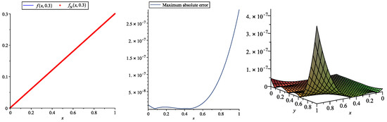
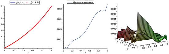
Figure 1. Plots of the exact and approximate solutions (left), maximum absolute error (middle) at $y=0.3$, and absolute error (right) obtained by the 2D-SJPs with $N=3$ and $\tau =\varsigma =0$ for Example 1.

Example 2.

Consider the following 2D-NFIDE studied by [36]:

$$\begin{array}{cc}\hfill & f_{yy}(x,y)+f_{yx}(x,y)+f(x,y)+I^{(\frac{5}{2},1)}f(x,y)=g(x,y)+\rho (x,y)+\phi (x,y),\hfill \end{array}$$

with initial conditions

$$\begin{array}{cc}\hfill & f(x,0)=f_x(x,0)=f_y(x,0)=f_x(0,y)=0,f(0,y)={\displaystyle \frac{y^2}{4}},\hfill \end{array}$$

where $(x,y)\in [0,1)\times [0,1)$ and

$$\begin{array}{cc}\hfill & \rho (x,y)={\displaystyle \frac{1}{\mathsf{\Gamma }\left(\frac{5}{2}\right)\mathsf{\Gamma }\left(1\right)}}{\int }_0^1{\int }_0^1{(1-t)}^{\frac{3}{2}}{y}^{\frac{8}{3}}{x}^{\frac{7}{2}}{t}^{3}f(t,s)\mathrm{d}s\mathrm{d}t,\hfill \\ \hfill & \phi (x,y)={\int }_0^1{\int }_0^1{\displaystyle \frac{3360}{46}}xy(x+y)f^2(t,s)\mathrm{d}s\mathrm{d}t,\hfill \\ \hfill & g(x,y)=-{\displaystyle \frac{608}{153153\sqrt{\pi }}}{x}^{\frac{7}{2}}{y}^{\frac{8}{3}}+{\displaystyle \frac{1}{4}}(x^3+1)y^2+{\displaystyle \frac{1}{2}}(x^3+1)-{\displaystyle \frac{3}{2}}x{y}^2+{\displaystyle \frac{2(16x^3+231)x^{\frac{5}{2}}{y}^3}{10395\sqrt{\pi }}}.\hfill \end{array}$$

The exact solution is $f(x,y)={\displaystyle \frac{y^2}{4}}(x^3+1)$.

Table 4 and Table 5 report the obtained numerical results and absolute errors, respectively, using the new approach and choosing $\tau =\varsigma =0$ and $N=2,3$. Additionally, Table 6 reports maximum absolute errors by selecting various values of τ, ς and $N=2$. These tables show that by choosing $\mathfrak{B}={(N+1)}^2=16$ numbers of 2D-SJPs, our obtained results are more accurate than the results reported in [36,37] and use $\mathfrak{B}=N^2{M}^2=36$ and $\mathfrak{B}=m^2=1024$ numbers of 2D-HBPSLs and 2D-BPFs, respectively, for solving this problem. In Figure 2, the accuracy and efficiency of proposed method is illustrated.

Table 4. Numerical results with $\tau =\varsigma =0$ for Example 2.

$\mathit{x}\mathbf{=}\mathit{y}$	Exact Solution	2D-SJPs		2D-HBPSLs [37]	2D-BPFs [36]
		$\mathit{N}\mathbf{=}\mathbf{2}$	$\mathit{N}\mathbf{=}\mathbf{3}$	$\mathit{N}\mathbf{=}\mathbf{2}\mathbf{,}\mathit{M}\mathbf{=}\mathbf{3}$	$\mathit{m}\mathbf{=}\mathbf{32}$
		$\mathfrak{B}\mathbf{=}\mathbf{9}$	$\mathfrak{B}\mathbf{=}\mathbf{16}$	$\mathfrak{B}\mathbf{=}\mathbf{36}$	$\mathfrak{B}\mathbf{=}\mathbf{1024}$
0	0	$3.50087\times {10}^{-8}$	$-1.75105\times {10}^{-11}$	$-1.70722\times {10}^{-8}$	$5.31008\times {10}^{-5}$
$0.2$	$0.01008$	$0.00990005$	$0.01008$	$0.0100625$	$9.04921\times {10}^{-3}$
$0.4$	$0.04256$	$0.0419991$	$0.04256$	$0.0426493$	$0.035166$
$0.6$	$0.10944$	$0.110691$	$0.10944$	$0.109233$	$0.099042$
$0.8$	$0.24192$	$0.244764$	$0.24192$	$0.242178$	$0.208004$
$0.99$	$0.482773$	$0.471861$	$0.482772$	$0.481524$	$0.411787$
Max error	0	$5.746197\times {10}^{-5}$	$4.748580\times {10}^{-8}$	$3.570347\times {10}^{-4}$	$7.0986\times {10}^{-2}$

Table 5. Absolute errors with $\tau =\varsigma =0$ for Example 2.

$\mathit{x}\mathbf{=}\mathit{y}$	2D-SJPs		2D-HBPSLs [37]
	$\mathit{N}\mathbf{=}\mathbf{2}$	$\mathit{N}\mathbf{=}\mathbf{3}$	$\mathit{N}\mathbf{=}\mathbf{2}\mathbf{,}\mathit{M}\mathbf{=}\mathbf{3}$
	$\mathfrak{B}\mathbf{=}\mathbf{9}$	$\mathfrak{B}\mathbf{=}\mathbf{16}$	$\mathfrak{B}\mathbf{=}\mathbf{36}$
0	$3.500869\times {10}^{-8}$	$1.751047\times {10}^{-11}$	$1.707223\times {10}^{-8}$
$0.1$	$9.992949\times {10}^{-6}$	$1.282426\times {10}^{-12}$	$5.623240\times {10}^{-6}$
$0.2$	$1.799480\times {10}^{-4}$	$1.250557\times {10}^{-11}$	$1.752097\times {10}^{-5}$
$0.3$	$4.950320\times {10}^{-4}$	$7.129280\times {10}^{-11}$	$3.919885\times {10}^{-5}$
$0.4$	$5.608532\times {10}^{-4}$	$3.100506\times {10}^{-10}$	$8.934775\times {10}^{-5}$
$0.5$	$3.355656\times {10}^{-6}$	$1.029452\times {10}^{-9}$	$3.884051\times {10}^{-4}$
$0.6$	$1.251167\times {10}^{-3}$	$2.924318\times {10}^{-9}$	$2.071935\times {10}^{-4}$
$0.7$	$2.676069\times {10}^{-3}$	$7.479405\times {10}^{-9}$	$2.249140\times {10}^{-4}$
$0.8$	$2.844359\times {10}^{-3}$	$1.753510\times {10}^{-8}$	$2.583723\times {10}^{-4}$
$0.9$	$8.713086\times {10}^{-4}$	$7.185571\times {10}^{-8}$	$4.152332\times {10}^{-4}$

Table 6. Maximum absolute errors with $N=2$ for Example 2.

$\mathbf{(}\mathsf{\tau }\mathbf{,}\mathsf{\varsigma }\mathbf{)}$	$\mathit{M}\mathit{A}\mathit{E}$	$\mathbf{(}\mathsf{\tau }\mathbf{,}\mathsf{\varsigma }\mathbf{)}$	$\mathit{M}\mathit{A}\mathit{E}$
$(0,0)$	$5.746197\times {10}^{-5}$	$(1,1)$	$2.502457\times {10}^{-3}$
$(1,2)$	$2.374060\times {10}^{-2}$	$(2,1)$	$1.116405\times {10}^{-2}$
$(2,2)$	$3.419813\times {10}^{-3}$	$(3,2)$	$9.826693\times {10}^{-3}$

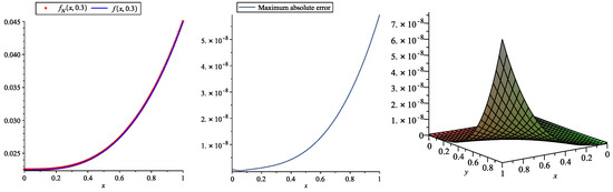
Figure 2. Plots of the exact and approximate solutions (left), maximum absolute error (middle) at $y=0.3$, and absolute error (right) obtained by the 2D-SJPs with $N=3$ and $\tau =\varsigma =0$ for Example 2.

Example 3.

Consider the following 2D-NFIDE:

$$\begin{array}{cc}\hfill & f_{yy}(x,y)+f_{yx}(x,y)+f(x,y)=g(x,y)+\rho (x,y),\hfill \end{array}$$

with initial conditions

$$\begin{array}{cc}\hfill & f(x,0)=f_x(x,0)=f_y(x,0)={\mathrm{e}}^x,f(0,y)={\mathrm{e}}^y,\hfill \end{array}$$

where $(x,y)\in [0,2)\times [0,2)$

$$\begin{array}{cc}\hfill & \rho (x,y)={\displaystyle \frac{1}{\mathsf{\Gamma }\left(\frac{3}{2}\right)\mathsf{\Gamma }\left(\frac{3}{2}\right)}}{\int }_0^2{\int }_0^2{(2-t)}^{\frac{1}{2}}{(2-s)}^{\frac{1}{2}}(x+y)(t^2+s^2)f(t,s)\mathrm{d}s\mathrm{d}t,\hfill \\ \hfill & g(x,y)=3{\mathrm{e}}^{x+y}-4(x+y)\left(\frac{11}{\pi }-\frac{9{\mathrm{e}}^2\sqrt{2}\mathrm{erf}\left(\sqrt{2}\right)}{\sqrt{\pi }}+\frac{7{\mathrm{e}}^4{\left(\mathrm{erf}\left(\sqrt{2}\right)\right)}^2}{8}\right).\hfill \end{array}$$

The exact solution is $f(x,y)={\mathrm{e}}^{x+y}$. Note that $\mathrm{erf}\left(x\right)=\frac{2{\int }_0^x{\mathrm{e}}^{-x^2}\mathrm{d}x}{\sqrt{\pi }}$.

Table 7 and Table 8 report the obtained numerical results and absolute errors, respectively, using the new approach and choosing $\tau =\varsigma =0$ and $N=4,5$. These tables show that by choosing $\mathfrak{B}={(N+1)}^2=36$ numbers of 2D-SJPs, our obtained results are more accurate than the results reported in [37] and use $\mathfrak{B}=N^2{M}^2=64$ numbers of 2D-HBPSLs for solving this problem. From Figure 3, the accuracy and efficiency of the proposed method is illustrated.

Table 7. Numerical results with $\tau =\varsigma =0$ for Example 3.

$\mathit{x}\mathbf{=}\mathit{y}$	Exact Solution	2D-SJPs		2D-HBPSLs [37]
		$\mathit{N}\mathbf{=}\mathbf{4}$	$\mathit{N}\mathbf{=}\mathbf{5}$	$\mathit{N}\mathbf{=}\mathbf{2}\mathbf{,}\mathit{M}\mathbf{=}\mathbf{4}$
		$\mathfrak{B}\mathbf{=}\mathbf{25}$	$\mathfrak{B}\mathbf{=}\mathbf{36}$	$\mathfrak{B}\mathbf{=}\mathbf{64}$
0	1	$0.999498$	$1.00004$	$0.99811$
$0.2$	$1.49182$	$1.49209$	$1.49181$	$1.49284$
$0.4$	$2.22554$	$2.22543$	$2.22556$	$2.22493$
$0.6$	$3.32012$	$3.31979$	$3.32012$	$3.31909$
$0.8$	$4.95303$	$4.95305$	$4.953$	$4.95461$
1	$7.38906$	$7.38946$	$7.38905$	$7.37414$
$1.2$	$11.0232$	$11.0233$	$11.0232$	$11.0301$
$1.4$	$16.4446$	$16.4439$	$16.4446$	$16.4394$
$1.6$	$24.5325$	$24.5318$	$24.5325$	$24.5242$
$1.8$	$36.5982$	$36.5992$	$36.5983$	$36.6095$
Max error	0	$3.352898\times {10}^{-4}$	$2.293543\times {10}^{-5}$	$1.118645\times {10}^{-2}$

Table 8. Absolute errors with $\tau =\varsigma =0$ for Example 3.

$\mathit{x}\mathbf{=}\mathit{y}$	2D-SJPs		2D-HBPSLs [37]
	$\mathit{N}\mathbf{=}\mathbf{4}$	$\mathit{N}\mathbf{=}\mathbf{5}$	$\mathit{N}\mathbf{=}\mathbf{2}\mathbf{,}\mathit{M}\mathbf{=}\mathbf{4}$
	$\mathfrak{B}\mathbf{=}\mathbf{25}$	$\mathfrak{B}\mathbf{=}\mathbf{36}$	$\mathfrak{B}\mathbf{=}\mathbf{64}$
0	$5.018269\times {10}^{-4}$	$3.878596\times {10}^{-5}$	$1.890271\times {10}^{-3}$
$0.2$	$2.646095\times {10}^{-4}$	$1.323019\times {10}^{-5}$	$1.016898\times {10}^{-3}$
$0.4$	$1.156163\times {10}^{-4}$	$1.971321\times {10}^{-5}$	$6.116798\times {10}^{-4}$
$0.6$	$3.222169\times {10}^{-4}$	$1.006197\times {10}^{-6}$	$1.030940\times {10}^{-3}$
$0.8$	$1.401881\times {10}^{-5}$	$2.886721\times {10}^{-5}$	$1.578274\times {10}^{-3}$
1	$4.053898\times {10}^{-4}$	$7.535908\times {10}^{-6}$	$1.491810\times {10}^{-2}$
$1.2$	$1.410474\times {10}^{-4}$	$3.456475\times {10}^{-5}$	$6.949542\times {10}^{-3}$
$1.4$	$7.246987\times {10}^{-4}$	$6.085008\times {10}^{-7}$	$5.233810\times {10}^{-3}$
$1.6$	$7.533610\times {10}^{-4}$	$7.863965\times {10}^{-5}$	$8.312774\times {10}^{-3}$
$1.8$	$9.833575\times {10}^{-4}$	$3.723796\times {10}^{-5}$	$1.126113\times {10}^{-2}$

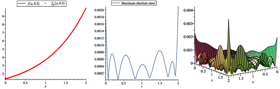
Figure 3. Plots of the exact and approximate solutions (left), maximum absolute error (middle) at $y=0.3$, and absolute error (right) obtained by the 2D-SJPs with $N=5$ and $\tau =\varsigma =0$ for Example 3.

Example 4.

Consider the following 2D-NFIDE:

$$\begin{array}{cc}\hfill & f_{xx}(x,y)+f(x,y)+I^{(\frac{3}{2},1)}f(x,y)=g(x,y)+\Theta (x,y),\hfill \end{array}$$

with initial conditions

$$\begin{array}{cc}\hfill & f(x,0)=f(0,y)=f_y(x,0)=f_x(0,y)=f_x(x,0)=0,\hfill \end{array}$$

where $(x,y)\in [0,1)\times [0,1)$ and

$$\begin{array}{cc}\hfill \Theta (x,y)=& {\int }_0^x{\int }_0^y(yt-xs)f^2(t,s)\mathrm{d}s\mathrm{d}t,\hfill \\ \hfill g(x,y)=& -\frac{1}{360{\pi }^{\frac{9}{2}}}\left(y((-360x^2-720)sin\left(\pi y\right)+x^6{y}^3){\pi }^{\frac{9}{2}}+24y^2\left(cos{\left(\pi y\right)}^2-\frac{1}{2}\right)x^6{\pi }^{\frac{5}{2}}\right.\hfill \\ \hfill & +\frac{768{\pi }^2\left(\pi ycos\left(\pi y\right)-sin\left(\pi y\right)\right)x^{\frac{7}{2}}}{7}\hfill \\ \hfill & -27x^6\left(\frac{1}{9}{\pi }^{\frac{3}{2}}ysin\left(\pi y\right)cos\left(\pi y\right)\left(-2{\pi }^2{y}^2+13\right)+cos{\left(\pi y\right)}^2\sqrt{\pi }-\sqrt{\pi }\right).\hfill \end{array}$$

The exact solution is $f(x,y)=x^{2}ysin\left(\pi y\right)$.

Table 9 and Table 10 report the obtained numerical results and absolute errors, respectively, using the new approach and choosing $\tau =\varsigma =0$ and $N=3,4$. Additionally, Table 11 reports maximum absolute errors by selecting various values of τ, ς and $N=2$. These tables show that by choosing $\mathfrak{B}={(N+1)}^2=25$ numbers of 2D-SJPs, our obtained results are more accurate than the results obtained by the 2D-HBPSL method [37] and use $\mathfrak{B}=N^2{M}^2=36$ bases for solving this problem. In Figure 4, the accuracy and efficiency of the proposed method is illustrated.

Table 9. Numerical results with $\tau =\varsigma =0$ for Example 4.

$\mathit{x}\mathbf{=}\mathit{y}$	Exact Solution	2D-SJPs		2D-HBPSLs [37]
		$\mathit{N}\mathbf{=}\mathbf{3}$	$\mathit{N}\mathbf{=}\mathbf{4}$	$\mathit{M}\mathbf{=}\mathit{N}\mathbf{=}\mathbf{2}$	$\mathit{N}\mathbf{=}\mathbf{2}\mathbf{,}\mathit{M}\mathbf{=}\mathbf{3}$
		$\mathfrak{B}=\mathbf{16}$	$\mathfrak{B}=\mathbf{25}$	$\mathfrak{B}=\mathbf{16}$	$\mathfrak{B}=\mathbf{36}$
0	0	$1.42563\times {10}^{-6}$	$-1.53250\times {10}^{-7}$	$0.00304418$	$-5.40176\times {10}^{-8}$
$0.2$	$0.00470228$	$0.00503905$	$0.00461625$	$0.00860387$	$0.00502286$
$0.4$	$0.0608676$	$0.0606074$	$0.0615685$	$0.0582732$	$0.0592075$
$0.6$	$0.205428$	$0.201651$	$0.203813$	$0.2084$	$0.206665$
$0.8$	$0.300946$	$0.309229$	$0.302467$	$0.253177$	$0.299392$
Max error	0	$4.183049\times {10}^{-3}$	$2.691559\times {10}^{-4}$	$1.686288\times {10}^{-2}$	$6.519558\times {10}^{-3}$

Table 10. Absolute errors with $\tau =\varsigma =0$ for Example 4.

$\mathit{x}\mathbf{=}\mathit{y}$	2D-SJPs		2D-HBPSLs [37]
	$\mathit{N}\mathbf{=}\mathbf{3}$	$\mathit{N}\mathbf{=}\mathbf{4}$	$\mathit{M}\mathbf{=}\mathit{N}\mathbf{=}\mathbf{2}$	$\mathit{N}\mathbf{=}\mathbf{2}\mathbf{,}\mathit{M}\mathbf{=}\mathbf{3}$
	$\mathfrak{B}\mathbf{=}\mathbf{16}$	$\mathfrak{B}\mathbf{=}\mathbf{25}$	$\mathfrak{B}\mathbf{=}\mathbf{16}$	$\mathfrak{B}\mathbf{=}\mathbf{36}$
0	$1.425634\times {10}^{-6}$	$1.532497\times {10}^{-7}$	$3.044182\times {10}^{-3}$	$5.401763\times {10}^{-8}$
$0.1$	$2.359796\times {10}^{-6}$	$5.799964\times {10}^{-5}$	$1.304790\times {10}^{-6}$	$8.310324\times {10}^{-5}$
$0.2$	$3.367631\times {10}^{-4}$	$8.603064\times {10}^{-5}$	$3.901591\times {10}^{-3}$	$3.205808\times {10}^{-4}$
$0.3$	$6.244970\times {10}^{-4}$	$3.609740\times {10}^{-4}$	$6.081376\times {10}^{-3}$	$6.170073\times {10}^{-4}$
$0.4$	$2.601698\times {10}^{-4}$	$7.008446\times {10}^{-4}$	$2.594409\times {10}^{-3}$	$1.660119\times {10}^{-3}$
$0.5$	$2.479625\times {10}^{-3}$	$5.263376\times {10}^{-5}$	$1.670057\times {10}^{-2}$	$2.207590\times {10}^{-3}$
$0.6$	$3.776819\times {10}^{-3}$	$1.615412\times {10}^{-3}$	$2.972021\times {10}^{-3}$	$1.236545\times {10}^{-3}$
$0.7$	$3.370614\times {10}^{-4}$	$1.772158\times {10}^{-3}$	$3.193363\times {10}^{-2}$	$1.625204\times {10}^{-5}$
$0.8$	$8.282794\times {10}^{-3}$	$1.521422\times {10}^{-3}$	$4.776857\times {10}^{-2}$	$1.553977\times {10}^{-3}$
$0.9$	$9.162584\times {10}^{-3}$	$4.275932\times {10}^{-3}$	$5.981687\times {10}^{-3}$	$4.222491\times {10}^{-4}$

Table 11. Maximum absolute errors with $N=2$ for Example 4.

$\mathbf{(}\mathsf{\tau }\mathbf{,}\mathsf{\varsigma }\mathbf{)}$	$\mathit{M}\mathit{A}\mathit{E}$	$\mathbf{(}\mathsf{\tau }\mathbf{,}\mathsf{\varsigma }\mathbf{)}$	$\mathit{M}\mathit{A}\mathit{E}$
$(0,0)$	$4.183049\times {10}^{-3}$	$(1,1)$	$7.254076\times {10}^{-3}$
$(1,2)$	$6.743181\times {10}^{-3}$	$(2,1)$	$4.492349\times {10}^{-3}$
$(2,2)$	$4.903053\times {10}^{-3}$	$(3,2)$	$3.081034\times {10}^{-3}$

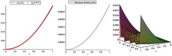
Figure 4. Plots of the exact and approximate solutions (left), maximum absolute error (middle) at $y=0.3$, and absolute error (right) obtained by the 2D-SJPs with $N=4$ and $\tau =\varsigma =0$ for Example 4.

Example 5.

Consider the following 2D-NFIDE:

$$\begin{array}{cc}\hfill & f_{yy}(x,y)+f_{yx}(x,y)+f(x,y)+I^{(\frac{3}{2},1)}f(x,y)=g(x,y)+\Theta (x,y)+\phi (x,y),\hfill \end{array}$$

with initial conditions

$$\begin{array}{cc}\hfill & f(x,0)=0,f(0,y)=sin\left(\pi y\right),f_y(x,0)=\pi {\mathrm{e}}^x,f_x(0,y)=sin\left(\pi y\right),f_x(x,0)=0,\hfill \end{array}$$

where $(x,y)\in [0,1)\times [0,1)$ and

$$\begin{array}{cc}\hfill & \Theta (x,y)={\int }_0^x{\int }_0^{y}xys{f}^2(t,s)\mathrm{d}s\mathrm{d}t,\hfill \\ \hfill & \phi (x,y)={\int }_0^1{\int }_0^1{x}^2{y}^3{t}^2{f}^2(t,s)\mathrm{d}s\mathrm{d}t,\hfill \\ \hfill & g(x,y)=-\frac{1}{8{\pi }^{\frac{5}{2}}}\left(\left(x{y}^2\left(x-\frac{1}{2}\right){\mathrm{e}}^{2x}+{\mathrm{e}}^2{x}^2{y}^3-x^2{y}^3+\frac{1}{2}x{y}^2\right.-8{\mathrm{e}}^{x}sin\left(\pi y\right)\right){\pi }^{\frac{5}{2}}\hfill \\ \hfill & +\left(\left(-2sin\left(\pi y\right)yx\left(x-\frac{1}{2}\right){\mathrm{e}}^{2x}-sin\left(\pi y\right)yx+8{\mathrm{e}}^x\mathrm{erf}\left(\sqrt{x}\right)\right)cos\left(\pi y\right)-8{\mathrm{e}}^x\mathrm{erf}\left(\sqrt{x}\right)\right){\pi }^{\frac{3}{2}}\hfill \\ \hfill & -8{\pi }^{\frac{7}{2}}{\mathrm{e}}^{x}cos\left(\pi y\right)+8{\pi }^{\frac{9}{2}}{\mathrm{e}}^{x}sin\left(\pi y\right)-(-1+cos\left(\pi y\right))\left(x\left(\frac{1}{2}+\left(x-\frac{1}{2}\right){\mathrm{e}}^{2x}\right)\sqrt{\pi }cos\left(\pi y\right)\right.\hfill \\ \hfill & \left.\left.+x\sqrt{\pi }\left(x-\frac{1}{2}\right){\mathrm{e}}^{2x}+\frac{1}{2}x\sqrt{\pi }+16\pi \sqrt{x}\right)\right).\hfill \end{array}$$

The exact solution is $f(x,y)={\mathrm{e}}^{x}sin\left(\pi y\right)$.

Table 12 and Table 13 report the obtained numerical results and absolute errors, respectively, using the new approach and choosing $\tau =\varsigma =0$ and $N=3,4$. Additionally, Table 14 reports maximum absolute errors by selecting various values of τ, ς and $N=3$. These tables show that by choosing $\mathfrak{B}={(N+1)}^2=25$ numbers of 2D-SJPs, our obtained results are more accurate than the results obtained by the 2D-HBPSL method [37] and use $\mathfrak{B}=N^2{M}^2=36$ bases for solving this problem. In Figure 5, the accuracy and efficiency of proposed method is illustrated.

Table 12. Numerical results with $\tau =\varsigma =0$ for Example 5.

$\mathit{x}\mathbf{=}\mathit{y}$	Exact Solution	2D-SJPs		2D-HBPSLs [37]
		$\mathit{N}\mathbf{=}\mathbf{3}$	$\mathit{N}\mathbf{=}\mathbf{4}$	$\mathit{M}\mathbf{=}\mathit{N}\mathbf{=}\mathbf{2}$	$\mathit{N}\mathbf{=}\mathbf{2}\mathbf{,}\mathit{M}\mathbf{=}\mathbf{3}$
		$\mathfrak{B}\mathbf{=}\mathbf{16}$	$\mathfrak{B}\mathbf{=}\mathbf{25}$	$\mathfrak{B}\mathbf{=}\mathbf{16}$	$\mathfrak{B}\mathbf{=}\mathbf{36}$
0	0	$-0.0498894$	$0.00126408$	$0.106466$	$-0.0269479$
$0.2$	$0.717923$	$0.743648$	$0.718851$	$0.644168$	$0.713975$
$0.4$	$1.41881$	$1.39875$	$1.41815$	$1.33223$	$1.3479$
$0.6$	$1.73294$	$1.70905$	$1.73227$	$1.43579$	$1.40505$
$0.8$	$1.30814$	$1.35737$	$1.31117$	$0.694829$	$0.506292$
Max error	0	$4.900771\times {10}^{-3}$	$2.890626\times {10}^{-3}$	$7.161353\times {10}^{-1}$	$1.625743$

Table 13. Absolute errors with $\tau =\varsigma =0$ for Example 5.

$\mathit{x}\mathbf{=}\mathit{y}$	2D-SJPs		2D-HBPSLs [37]
	$\mathit{N}\mathbf{=}\mathbf{3}$	$\mathit{N}\mathbf{=}\mathbf{4}$	$\mathit{M}\mathbf{=}\mathit{N}\mathbf{=}\mathbf{2}$	$\mathit{N}\mathbf{=}\mathbf{2}\mathbf{,}\mathit{M}\mathbf{=}\mathbf{3}$
	$\mathfrak{B}\mathbf{=}\mathbf{16}$	$\mathfrak{B}\mathbf{=}\mathbf{25}$	$\mathfrak{B}\mathbf{=}\mathbf{16}$	$\mathfrak{B}\mathbf{=}\mathbf{36}$
0	$4.988938\times {10}^{-2}$	$1.264079\times {10}^{-3}$	$1.064657\times {10}^{-1}$	$2.694793\times {10}^{-2}$
$0.1$	$1.314614\times {10}^{-2}$	$2.544488\times {10}^{-4}$	$1.500519\times {10}^{-2}$	$7.810507\times {10}^{-3}$
$0.2$	$2.572567\times {10}^{-2}$	$9.282027\times {10}^{-4}$	$7.375466\times {10}^{-2}$	$3.947639\times {10}^{-3}$
$0.3$	$7.178138\times {10}^{-3}$	$6.978147\times {10}^{-4}$	$1.226548\times {10}^{-1}$	$3.448407\times {10}^{-2}$
$0.4$	$2.005857\times {10}^{-2}$	$6.560525\times {10}^{-4}$	$8.657965\times {10}^{-2}$	$7.090727\times {10}^{-2}$
$0.5$	$3.495032\times {10}^{-2}$	$1.518547\times {10}^{-3}$	$1.553134\times {10}^{-1}$	$3.482695\times {10}^{-1}$
$0.6$	$2.389001\times {10}^{-2}$	$6.632893\times {10}^{-4}$	$2.971477\times {10}^{-1}$	$3.278872\times {10}^{-1}$
$0.7$	$1.206528\times {10}^{-2}$	$1.561235\times {10}^{-3}$	$4.595629\times {10}^{-1}$	$5.951170\times {10}^{-1}$
$0.8$	$4.922751\times {10}^{-2}$	$3.025826\times {10}^{-3}$	$6.133115\times {10}^{-1}$	$8.018483\times {10}^{-1}$
$0.9$	$3.323691\times {10}^{-2}$	$2.322792\times {10}^{-3}$	$7.485747\times {10}^{-1}$	$1.408296$

Table 14. Maximum absolute errors with $N=3$ for Example 5.

$\mathbf{(}\mathsf{\tau }\mathbf{,}\mathsf{\varsigma }\mathbf{)}$	$\mathit{M}\mathit{A}\mathit{E}$	$\mathbf{(}\mathsf{\tau }\mathbf{,}\mathsf{\varsigma }\mathbf{)}$	$\mathit{M}\mathit{A}\mathit{E}$
$(0,0)$	$4.90077\times {10}^{-3}$	$(1,1)$	$3.494379\times {10}^{-2}$
$(1,2)$	$1.159618\times {10}^{-1}$	$(2,1)$	$1.718043\times {10}^{-2}$
$(2,2)$	$6.089228\times {10}^{-2}$	$(3,2)$	$3.330454\times {10}^{-2}$

Figure 5. Plots of the exact and approximate solutions (left), maximum absolute error (middle) at $y=0.3$, and absolute error (right) obtained by the 2D-SJPs with $N=4$ and $\tau =\varsigma =0$ for Example 5.

7. Conclusions

In this research, sufficient conditions for the existence and uniqueness of local and global solutions of general 2D-NFIDEs were provided. Additionally, the collocation method and operational matrices based on 2D-SJPs were used for solving these equations. Moreover, error bounds of the proposed method were obtained. We showed that the order of convergence of the method is $O\left({\displaystyle \frac{1}{{\left(N(N+\tau +\varsigma )\right)}^{\frac{\epsilon -ϵ}{2}}}}\right)$ in the Jacobi-weighted Sobolev space. Finally, we evaluated the presented method by solving five test problems. The obtained numerical results showed that a favorable approximate solution can be obtained by using lower numbers of basis functions.

References

- Atangana, A.; Kılıçman, A. A possible generalization of acoustic wave equation using the concept of perturbed derivative order. Math. Probl. Eng. 2013, 2013, 696597. [Google Scholar] [CrossRef]
- Atangana, A.; Kılıçman, A. Analytical solutions of the spacetime fractional derivative of advection dispersion equation. Math. Probl. Eng. 2013, 2013, 853127. [Google Scholar] [CrossRef]
- Benson, D.A.; Wheatcraft, S.W.; Meerschaert, M.M. Application of a fractional advection-dispersion equation. Water Resour. Res. 2000, 36, 1403–1412. [Google Scholar] [CrossRef]
- Caputo, M. Linear models of dissipation whose Q is almost frequency independent-part II. Geophys. J. Int. 1967, 13, 529–539. [Google Scholar] [CrossRef]
- Cloot, A.; Botha, J.F. A generalised groundwater flow equation using the concept of non-integer order derivatives. Water SA 2006, 32, 55–78. [Google Scholar] [CrossRef]
- Meerschaert, M.M.; Tadjeran, C. Finite difference approximations for fractional advection-dispersion flow equations. J. Comput. Appl. Math. 2004, 172, 65–77. [Google Scholar] [CrossRef]
- Chen, C.M.; Liu, F.; Turner, I.; Anh, V. A Fourier method for the fractional diffusion equation describing sub-diffusion. J. Comput. Phys. 2007, 227, 886–897. [Google Scholar] [CrossRef]
- Mainardi, F. Fractional calculus: Some basic problems in continuum and statistical mechanics. In Fractals and Fractional Calculus in Continuum Mechanics; Carpinteri, A., Mainardi, F., Eds.; Springer: New York, NY, USA, 1997; pp. 291–348. [Google Scholar]
- Yuste, S.B.; Acedo, L. An explicit finite difference method and a new von Neumann-type stability analysis for fractional diffusion equations. SIAM J. Numer. Anal. 2005, 42, 1862–1874. [Google Scholar] [CrossRef]
- Zhuang, P.; Liu, F.; Anh, V.; Turner, I. Numerical methods for the variable-order fractional advection-diffusion equation with a nonlinear source term. SIAM J. Numer. Anal. 2009, 47, 1760–1781. [Google Scholar] [CrossRef]
- Carpinteri, A.; Mainardi, F. Fractals and Fractional Calculus in Continuum Mechanics; Springer: New York, NY, USA, 1997; pp. 223–276. [Google Scholar]
- Metzler, F.; Schick, W.; Kilian, H.G.; Nonnenmacher, T.F. Relaxation in filled polymers: A fractional calculus approach. J. Chem. Phys. 1995, 103, 7180–7186. [Google Scholar] [CrossRef]
- Oldham, K.B.; Spanier, J. The Fractional Calculus; Academic Press: New York, NY, USA; London, UK, 1974. [Google Scholar]
- Thomas, R.; Fehmi, C. An immersed finite element method with integral equation correction. Int. J. Numer. Methods Eng. 2010, 86, 93–114. [Google Scholar]
- Taheri, Z.; Javadi, S.; Babolian, E. Numerical solution of stochastic fractional integro-differential equation by the spectral collocation method. J. Comput. Appl. Math. 2017, 321, 336–347. [Google Scholar] [CrossRef]
- Rahimkhania, P.; Ordokhani, Y.; Babolian, E. A numerical scheme for solving nonlinear fractional Volterra integro-differential equations. Iran. J. Math. Sci. Inform. 2018, 13, 111–132. [Google Scholar]
- Wang, Y.; Zhu, L.; Wang, Z. Fractional-order Euler functions for solving fractional integro-differential equations with weakly singular kernel. Adv. Differ. Equ. 2018, 2018, 254. [Google Scholar] [CrossRef]
- Babaei, A.; Jafari, H.; Banihashemi, S. Numerical solution of variable order fractional nonlinear quadratic integro-differential equations based on the sixth-kind Chebyshev collocation method. J. Comput. Appl. Math. 2020, 377, 112908. [Google Scholar] [CrossRef]
- Abbas, S.; Benchohra, M. Fractional order integral equations of two independent variables. Appl. Math. Comput. 2014, 227, 755–761. [Google Scholar] [CrossRef]
- Asgari, M.; Ezzati, R.; Jafari, H. Solution of 2D Fractional Order Integral Equations by Bernstein Polynomials Operational Matrices. Nonlinear Dyn. Syst. Theory 2019, 19, 10–20. [Google Scholar]
- Babolian, E.; Maleknejad, K.; Roodaki, M.; Almasieh, H. Two-dimensional triangular functions and their applications to nonlinear 2d Volterra-Fredholm integral equations. Comput. Math. Appl. 2010, 60, 1711–1722. [Google Scholar] [CrossRef]
- Eftekhari, T.; Hosseini, S.M. A new and efficient approach for solving linear and nonlinear time-fractional diffusion equations of distributed-order. Comput. Appl. Math. 2022, 41, 281. [Google Scholar] [CrossRef]
- Eftekhari, T.; Rashidinia, J. A novel and efficient operational matrix for solving nonlinear stochastic differential equations driven by multi-fractional Gaussian noise. Appl. Math. Comput. 2022, 429, 127218. [Google Scholar] [CrossRef]
- Eftekhari, T.; Rashidinia, J. A new operational vector approach for time-fractional subdiffusion equations of distributed order based on hybrid functions. Math. Methods Appl. Sci. 2022. [Google Scholar] [CrossRef]
- Eftekhari, T.; Rashidinia, J.; Maleknejad, K. Existence, uniqueness, and approximate solutions for the general nonlinear distributed-order fractional differential equations in a Banach space. Adv. Differ. Equ. 2021, 2021, 461. [Google Scholar] [CrossRef]
- Hesameddini, E.; Shahbazi, M. Two-dimensional shifted Legendre polynomials operational matrix method for solving the two-dimensional integral equations of fractional order. Appl. Math. Comput. 2018, 322, 40–54. [Google Scholar] [CrossRef]
- Khalil, H.; Khan, R.A. The use of Jacobi polynomials in the numerical solution of coupled system of fractional differential equations. Int. J. Comput. Math. 2015, 92, 1452–1472. [Google Scholar] [CrossRef]
- Maleknejad, K.; Rashidinia, J.; Eftekhari, T. A new and efficient numerical method based on shifted fractional-order Jacobi operational matrices for solving some classes of two-dimensional nonlinear fractional integral equations. Numer. Methods Partial Differ. Equ. 2021, 37, 2687–2713. [Google Scholar] [CrossRef]
- Maleknejad, K.; Rashidinia, J.; Eftekhari, T. Numerical solutions of distributed order fractional differential equations in the time domain using the Müntz-Legendre wavelets approach. Numer. Methods Partial Differ. Equ. 2021, 37, 707–731. [Google Scholar] [CrossRef]
- Maleknejad, K.; Rashidinia, J.; Eftekhari, T. Existence, uniqueness, and numerical analysis of solutions for some classes of two-dimensional nonlinear fractional integral equations in a Banach space. Comput. Appl. Math. 2020, 39, 271. [Google Scholar] [CrossRef]
- Maleknejad, K.; Rashidinia, J.; Eftekhari, T. Numerical solution of three-dimensional Volterra-Fredholm integral equations of the first and second kinds based on Bernstein’s approximation. Appl. Math. Comput. 2018, 339, 272–285. [Google Scholar] [CrossRef]
- Mirzaee, F.; Samadyar, N. Numerical solution based on two-dimensional orthonormal Bernstein polynomials for solving some classes of two-dimensional nonlinear integral equations of fractional order. Appl. Math. Comput. 2019, 344, 191–203. [Google Scholar] [CrossRef]
- Najafalizadeh, S.; Ezzati, R. Numerical methods for solving two-dimensional nonlinear integral equations of fractional order by using two-dimensional block pulse operational matrix. Appl. Math. Comput. 2016, 280, 46–56. [Google Scholar] [CrossRef]
- Rashidinia, J.; Eftekhari, T.; Maleknejad, K. Numerical solutions of two-dimensional nonlinear fractional Volterra and Fredholm integral equations using shifted Jacobi operational matrices via collocation method. J. King Saud Univ.-Sci. 2021, 33, 101244. [Google Scholar] [CrossRef]
- Rashidinia, J.; Eftekhari, T.; Maleknejad, K. A novel operational vector for solving the general form of distributed order fractional differential equations in the time domain based on the second kind Chebyshev wavelets. Numer. Algorithms 2021, 88, 1617–1639. [Google Scholar] [CrossRef]
- Najafalizadeh, S.; Ezzati, R. A block pulse operational matrix method for solving two-dimensional nonlinear integro-differential equations of fractional order. J. Comput. Appl. Math. 2017, 326, 159–170. [Google Scholar] [CrossRef]
- Maleknejad, K.; Rashidinia, J.; Eftekhari, T. Operational matrices based on hybrid functions for solving general nonlinear two-dimensional fractional integro-differential equations. Comp. Appl. Math. 2020, 39, 103. [Google Scholar] [CrossRef]
- Zeidler, E. Applied Functional Analysis: Applications to Mathematical Physics. Appl. Math. Sci. 1995, 108. [Google Scholar]
- Conway, J.B. A Course in Functional Analysis; Springer: Berlin/Heidelberg, Germany, 2007. [Google Scholar]
- Borhanifar, A.; Sadri, K. A Generalized Operational Method for Solving Integro-Partial Differential Equations Based on Jacobi Polynomials. Hacet. J. Math. Stat. 2016, 45, 311–335. [Google Scholar]
Disclaimer/Publisher’s Note: The statements, opinions and data contained in all publications are solely those of the individual author(s) and contributor(s) and not of MDPI and/or the editor(s). MDPI and/or the editor(s) disclaim responsibility for any injury to people or property resulting from any ideas, methods, instructions or products referred to in the content. |
© 2023 by the authors. Licensee MDPI, Basel, Switzerland. This article is an open access article distributed under the terms and conditions of the Creative Commons Attribution (CC BY) license (https://creativecommons.org/licenses/by/4.0/).