On Solvability Conditions for the Cauchy Problem for Non-Volterra Functional Differential Equations with Pointwise and Integral Restrictions on Functional Operators

Abstract

Cauchy problems are considered for families of, generally speaking, non-Volterra functional differential equations of the second order. For each family considered, in terms of the parameters of this family, necessary and sufficient conditions for the unique solvability of the Cauchy problem for all equations of the family are obtained. Such necessary and sufficient conditions are obtained for the following four kinds of families: integral restrictions are imposed on positive and negative functional operators, namely, operator norms are specified; pointwise restrictions are imposed on positive and negative functional operators in the form of values of operators’ actions on the unit function; an integral constraint is imposed on a positive functional operator, a pointwise constraint is imposed on a negative functional operator; a pointwise constraint is imposed on a positive functional operator, an integral constraint is imposed on a negative functional operator. In all cases, effective conditions for the solvability of the Cauchy problem for all equations of the family are obtained, expressed through some inequalities regarding the parameters of the families. The set of parameters of families of equations for which Cauchy problems are uniquely solvable can be easily calculated approximately with any accuracy. The resulting solvability conditions improve the solvability conditions following from the Banach contraction principle. An example of the Cauchy problem for an equation with a coefficient changing sign is given. Taking into account various restrictions for the positive and negative parts of functional operators allows us to significantly improve the known solvability conditions.

1. Preliminaries

The Cauchy problem for functional differential equations in the non-Volterra case [1] (§ 2.2.3, p. 50) has been studied quite intensively in recent years [1,2,3,4,5,6,7,8,9,10]. We consider the Cauchy problem for the linear second order functional differential equation

$$\begin{array}{c}\hfill \ddot{x}\left(t\right)=\left(T^{+}x\right)\left(t\right)-\left(T^{-}x\right)\left(t\right)+f\left(t\right),t\in [0,1],\end{array}$$

(1)

$$\begin{array}{c}\hfill x\left(0\right)=c_0,\dot{x}\left(0\right)=c_1,\end{array}$$

(2)

where the operators $T^{+}$, $T^{-}:\mathbf{C}[0,1]\to \mathbf{L}[0,1]$ are linear and positive, $f\in \mathbf{L}[0,1]$, $c_0$, $c_1\in \mathbb{R}$, $\mathbf{C}[0,1]$ and $\mathbf{L}[0,1]$ are the spaces of all continuous and integrable functions equipped with the standard norms respectively. An operator from $\mathbf{C}[0,1]$ into $\mathbf{L}[0,1]$ is called positive if it maps each non-negative function into an almost everywhere non-negative one. Equalities and inequalities with integrable functions will be considered as equalities and inequalities that are valid almost everywhere on the corresponding interval. Let ${\mathbf{AC}}^1[0,1]$ be the Banach space of all functions $x:[0,1]\to \mathbb{R}$ such that x and the derivative $\dot{x}$ are absolutely continuous on the interval $[0,1]$ with the norm ${\left|\right|x\left|\right|}_{{\mathbf{AC}}^1}=\left|x\left(0\right)\right|+|\dot{x}\left(0\right)|+{\int }_0^1\left|\ddot{x}\left(s\right)\right|ds$. We will say that a function $x:[0,1]\to \mathbb{R}$ is a solution to problem (1) and (2) if $x\in {\mathbf{AC}}^1[0,1]$, x satisfies Equation (1) almost everywhere on $[0,1]$, and x satisfies initial conditions (2).

In many results on solvability conditions for the Cauchy problem and other boundary value problems for functional differential equations, some smallness conditions are imposed on the positive part $T^{+}$ and the negative part $T^{-}$ of the functional operator $T=T^{+}-T^{-}$ (see [1,3,11,12,13,14,15]). Generally, the results are close to those obtained using the Banach contraction principle.

Using one-sided a priori estimates, A. Lomtatidze and S. Mukhigulashvili [16,17,18] managed to weaken the conditions on one of the operators $T^{+}$, $T^{-}$, guaranteeing the unique solvability of some boundary value problems. Similar relaxations of the solvability conditions were obtained by A. Lomtatidze, R. Hakl, B. Půža [19,20], A. Lomtatidze, R. Hakl, E. Bravyi [21] for the Cauchy problem, J. Šemr and R. Hakl [10,22,23] for the Cauchy problem for systems of functional differential equations, and by R. Hakl, A. Lomtatidze, S. Mukhigulashvili, B. Půža, for some other boundary value problems [16,24,25].

In these early works, integral restrictions were imposed on both functional operators in the form of integral inequalities

$${\int }_0^1\left(T^{+}\mathbf{1}\right)\left(s\right)ds⩽{\mathcal{P}}^{+},{\int }_0^1\left(T^{-}\mathbf{1}\right)\left(s\right)ds⩽{\mathcal{P}}^{-}$$

(see works on solvability conditions for the Cauchy problem [21] by A. Lomtatidze, R. Hakl, E. Bravyi and [10,19,20], where the solvability conditions for the operator $T^{-}$ were weakened and optimal solvability conditions for the Cauchy problem were obtained). Later, pointwise restrictions

$$\left(T^{+}\mathbf{1}\right)\left(t\right)⩽{\mathcal{P}}^{+},\left(T^{-}\mathbf{1}\right)\left(t\right)⩽{\mathcal{P}}^{-},t\in [0,1],$$

for some given constants ${\mathcal{P}}^{+}$, ${\mathcal{P}}^{-}$ were imposed on both functional operators [26] and the similar weaker solvability conditions on the operator $T^{-}$ were obtained.

However, apparently, for arbitrary pointwise constraints, necessary and sufficient solvability conditions for all equations in the family have not been obtained for a long time. But it is pointwise restrictions that give the narrowest families of equations and, therefore, the necessary and sufficient conditions for the solvability of the Cauchy problem for all equations from these families give the strongest results. Only in the work [27] were various types of pointwise constraints used to form families of equations.

Here we take a more general approach, using both types of constraints together (point and integral), so we get a new class of solvability conditions. And the obtained necessary and sufficient conditions for the solvability of the Cauchy problem for all equations from these families will exceed the known results.

We define new families of functional operators using two types of restrictions, integral for one from operators $T^{+}$, $T^{-}$ and pointwise restrictions for another operator. Then we find the necessary and sufficient conditions for a unique solvability of the Cauchy problem for all equations with operators from the chosen family. The obtained sufficient solvability conditions are unimprovable in the following sense. If these conditions are violated, then there exists an equation in the given family for which the Cauchy problem is not uniquely solvable.

All operators $T^{+}$ and $T^{-}$ considered here will belong to some families of the operators defined by pointwise and integral restrictions we impose on the functions $T^{+}\mathbf{1}$ and $T^{-}\mathbf{1}$, where $\mathbf{1}\left(t\right)=1$ is the unit function.

Let non-negative functions $p^{+}$, $p^{-}\in \mathbf{L}[0,1]$ and non-negative numbers ${\mathcal{P}}^{-}$, ${\mathcal{P}}^{+}$ be given. Let us introduce the following kinds of restrictions on the functional operators $T^{+}$ and $T^{-}$:

$$\left(T^{-}\mathbf{1}\right)\left(t\right)=p^{-}\left(t\right),t\in [0,1],\left(T^{+}\mathbf{1}\right)\left(t\right)=p^{+}\left(t\right),t\in [0,1],$$

(3)

$${\int }_0^1\left(T^{-}\mathbf{1}\right)\left(s\right)ds={\mathcal{P}}^{-},\left(T^{+}\mathbf{1}\right)\left(t\right)=p^{+}\left(t\right),t\in [0,1],$$

(4)

$$\left(T^{-}\mathbf{1}\right)\left(t\right)=p^{-}\left(t\right),t\in [0,1],{\int }_0^1\left(T^{+}\mathbf{1}\right)\left(s\right)ds={\mathcal{P}}^{+},$$

(5)

$${\int }_0^1\left(T^{-}\mathbf{1}\right)\left(s\right)ds={\mathcal{P}}^{-},{\int }_0^1\left(T^{+}\mathbf{1}\right)\left(s\right)ds={\mathcal{P}}^{+}.$$

(6)

Note that only conditions (3) [27] (it corresponds to pointwise restrictions) and conditions (6) [20,21,22,23,25,28,29] (corresponds to integral restrictions) were studied in earlier works (primarily in the case of the first order equations). The author is almost unaware of any works where mixed constraints (4) or (5) were used to obtain conditions for the solvability of the Cauchy problem (the only exception is the work [30], published during the preparation of this article).

Definition 1.

We will say that Cauchy problem (1) and (2) possesses the property ${\mathcal{A}}_i$, $i=1,2,3,4$, if problem (1) and (2) is uniquely solvable for all positive linear operators $T^{+}$, $T^{-}:\mathbf{C}[0,1]\to \mathbf{L}[0,1]$ satisfying conditions (3), (4), (5), (6) respectively.

In the study of boundary value problems for functional differential equations, the Fredholm property is often useful (see, for example, [1,3,31]). For the convenience of readers, we will give a definition of the Fredholm property and show that the Cauchy problem (1) and (2) possesses this property.

Below we present some information from [32]. Let $\mathbf{X}$, $\mathbf{Y}$ be Banach spaces, and $F:\mathbf{X}\to \mathbf{Y}$ a linear operator. The set of all solutions to the equation $Fx=0$ is called the null-space of the operator F. An operator F is called normal if the equation $Fx=y$ is solvable for those and only those $y\in \mathbf{Y}$ for which $g\left(y\right)=0$ for all solutions g of the homogeneous adjoint equation $F^{*}g=0$, where $F^{*}:{\mathbf{Y}}^{*}\to {\mathbf{X}}^{*}$ is the adjoint operator. For the operator F to be normal, it is necessary and sufficient that the range of values of the operator F be closed.

A normal operator is called Noetherian if it and its adjoint operator have null-spaces of finite dimension. The difference between those dimensions is called the operator index.

A Noetherian operator of zero index is called a Fredholm operator.

For a Fredholm operator F, the Fredholm alternative [31,32] is valid. In particular, the equation $Fx=g$ is uniquely solvable for all $g\in \mathbf{Y}$ if and only if the homogeneous equation $Fx=0$ has only the trivial solution.

For a bounded operator F to be Fredholm, it is necessary and sufficient that the operator F be representable in the form $F=W+V$, where the linear bounded operator $W:\mathbf{X}\to \mathbf{Y}$ is invertible, and the operator $V:\mathbf{X}\to \mathbf{Y}$ is completely continuous or finite-dimensional (we will call an operator with a finite-dimensional domain of values finite-dimensional). Thus, a finite-dimensional or completely continuous perturbation of the operator does not affect the Fredholm property.

Cauchy problem (1) and (2) can be rewritten in the form of one equation [5] (p. 14).

$$\left[\mathcal{L},\ell \right]x=\{f,c\},$$

where

$$\left(\mathcal{L}x\right)\left(t\right)\equiv \ddot{x}\left(t\right)-\left(\left(T^{+}x\right)\left(t\right)-\left(T^{-}x\right)\left(t\right)\right),t\in [0,1],$$

$$\ell x\equiv col\{x\left(0\right),\dot{x}\left(0\right)\}=col\{c_0,c_1\}\equiv c.$$

the linear operator $\left[\mathcal{L},\ell \right]$ acts from the space ${\mathbf{AC}}^1[0,1]$ into $\mathbf{L}[0,1]\times {\mathbb{R}}^2$.

Let us represent the operator $F=[\mathcal{L},\ell ]$ of the Cauchy problem (1) and (2) as

$$F=[\delta ,\ell ]-[T^{+}-T^{-},0],$$

where $\delta x=\ddot{x}$. Obviously, the operator

$$[\delta ,\ell ]:{\mathbf{AC}}^1[0,1]\to \mathbf{L}[0,1]\times {\mathbb{R}}^2$$

is invertible. Indeed, the Cauchy problem for the ordinary differential equation

$$\ddot{x}=f,x\left(0\right)=c_0,\dot{x}\left(0\right)=c_1$$

has a unique solution $x\left(t\right)={\int }_0^t(t-s)f\left(s\right)ds+c_0+t{c}_1$, $t\in [0,1]$.

Here we consider differences of linear positive operators $T^{+}$, $T^{-}:\mathbf{C}[0,1]\to \mathbf{L}[0,1]$. Each such operator is bounded. Indeed, the norm of the linear operator $T^{+}-T^{-}:\mathbf{C}[0,1]\to \mathbf{L}[0,1]$ is not greater than

$${\int }_0^1\left(\left(T^{+}\mathbf{1}\right)\left(t\right)+\left(T^{-}\mathbf{1}\right)\left(t\right)\right)dt,$$

where $\mathbf{1}\left(t\right)=1$, $t\in [0,1]$, is the unit function. Note that the norm of a positive operator $T^{+}:\mathbf{C}[0,1]\to \mathbf{L}[0,1]$ is equal to ${\int }_0^1\left(T^{+}\mathbf{1}\right)\left(t\right)dt$.

Further, the space ${\mathbf{AC}}^1[0,1]$ is compactly embedded into the space $\mathbf{C}[0,1]$. This can be proved by direct application of the Arzela–Ascoli theorem [31] (p. 27). Consequently, the bounded operator $T^{+}-T^{-}:\mathbf{C}[0,1]\to \mathbf{L}[0,1]$ is compact as an operator acting from the space ${\mathbf{AC}}^1[0,1]$ into the space $\mathbf{L}[0,1]$. Thus, the operator $[T^{+}-T^{-},0]:{\mathbf{AC}}^1[0,1]\to {\mathbb{R}}^2$ is compact. So, the operator $[\mathcal{L},\ell ]$ of the Cauchy problem (1) and (2) has the Fredholm property and the following assertion is valid.

Lemma 1 (The Fredholm alternative).

Cauchy problem (1) and (2) is uniquely solvable if and only if the homogeneous problem

$$\left\{\begin{array}{c}\ddot{x}\left(t\right)=\left(T^{+}x\right)\left(t\right)-\left(T^{-}x\right)\left(t\right),t\in [0,1],\hfill \\ x\left(0\right)=0,\dot{x}\left(0\right)=0,\hfill \end{array}\right.$$

(7)

has only the trivial solution.

The class of differences of linear positive operators from $\mathbf{C}[0,1]$ to $\mathbf{L}[0,1]$ includes operators with “deviated argument”:

$$\begin{array}{c}\hfill \left(Tx\right)\left(t\right)=\sum _{i=1}^m{p}_i\left(t\right)x_{h_i}\left(t\right),t\in [0,1],x_{h_i}\left(t\right)=\left\{\begin{array}{c}x\left(h_i\left(t\right)\right)\mathrm{if}{h}_i\left(t\right)\in [0,1],\hfill \\ 0\mathrm{if}{h}_i\left(t\right)\notin [0,1],\hfill \end{array}\right.\end{array}$$

where $p_i\in \mathbf{L}[0,1]$, $h_i:[0,1]\to \mathbb{R}$ are measurable functions, $i=1,\dots ,m$. These operators can be taken as illustrative examples for all statements of the work.

Note, every linear positive operator $T:\mathbf{C}[0,1]\to \mathbf{L}[0,1]$ has the representation [33] (pp. 303–304) in the form of the Riemann–Stieltjes integral:

$$\left(Tx\right)\left(t\right)={\int }_0^{1}x\left(s\right)d_{s}r(t,s),t\in [0,1],$$

where for each $t\in [0,1]$ the function $r(t,·)$ does not decrease, for each $s\in [0,1]$ the function $r(·,s)$ is integrable on $[0,1]$, $r(1,·)-r(0,·)\in \mathbf{L}[0,1]$.

Remark 1.

It is easy to see that all equalities in the definitions of properties ${\mathcal{A}}_i$, $i=1,2,3,4$, can be replaced by non-strict inequalities less than or equal to “⩽”.

Indeed, from the Fredholm property of the Cauchy problem (Lemma 1) it follows that it is sufficient to consider the homogeneous Cauchy problems. Then the unique solvability is equivalent to the absence of nontrivial solutions. If the problem does not possess some property in Definition 1, then it does not have this property for all greater or equal parameters. This follows from the fact that any additives in the form of a positive operator $\left(T_{0}x\right)\left(t\right)=q\left(t\right)x\left(0\right)$, $t\in [0,1]$, where $q\in \mathbf{L}[0,1]$, $q\left(t\right)⩾0$, $t\in [0,1]$, preserve a nontrivial solution to the homogeneous problem.

Our aim is to obtain necessary and sufficient conditions for the unique solvability of the Cauchy problem for all equations of the family to be uniquely solvable, that is, we search criteria for properties ${\mathcal{A}}_i$, $i=1,2,3,4$.

It should be emphasized that we consider generally speaking non-Volterra operators $T^{+}$, $T^{-}$, so the solvability of the Cauchy problem under natural assumptions is not guaranteed, unlike the Cauchy problem for ordinary differential equations. Note, the results can be used in the study of applied, in particular, computational problems such as in, for example [34,35]. The statements obtained in Theorems 1–4 improve all results known to the author (see [10,19,20,21,22,23,28,29,30]).

The work is organized as follows. Section 2 presents the main results. Section 3 contains a proof of Theorem 1. Section 4 contains proofs of Theorems 2 and 3 and Corollaries 1 and 2. Theorem 4 and Corollary 3 is proved in Section 5. Section 6 provides an example illustrating applications of Theorem 1. Section 7 discusses the results obtained.

2. Main Results

The main results are the following Theorems 1–4. In them we use the following notation

$$\begin{array}{c}\hfill {\Delta }_{-}(t_1,t_3,p^{-})\equiv \left(1+{\int }_0^{t_3}(1-s)p^{-}\left(s\right)ds\right)\left(1+{\int }_{t_3}^{t_1}(t_1-s)p^{-}\left(s\right)ds\right)-\\ \hfill {\int }_{t_3}^1(1-s)p^{-}\left(s\right)ds{\int }_0^{t_3}(t_1-s)p^{-}\left(s\right)ds,\end{array}$$

$$\begin{array}{c}\hfill {\Delta }_{+}(t_1,t_3,p^{+})\equiv \left(1-{\int }_0^{t_3}(t_1-s)p^{+}\left(s\right)ds\right)\left(1-{\int }_{t_3}^1(1-s)p^{+}\left(s\right)ds\right)-\\ \hfill {\int }_0^{t_3}(1-s)p^{+}\left(s\right)ds{\int }_{t_3}^{t_1}(t_1-s)p^{+}\left(s\right)ds,\end{array}$$

(8)

$$\begin{array}{c}\hfill {\Delta }_{+-}(t_1,t_3,p^{+},p^{-})\equiv {\int }_0^{t_3}(1-s)p^{+}\left(s\right)ds{\int }_0^{t_3}(t_1-s)p^{-}\left(s\right)ds-{\int }_0^{t_3}(t_1-s)p^{+}\left(s\right)ds{\int }_0^{t_3}(1-s)p^{-}\left(s\right)ds+\\ \hfill {\int }_{t_3}^{t_1}(t_1-s)p^{+}\left(s\right)ds{\int }_{t_3}^1(1-s)p^{-}\left(s\right)ds-{\int }_{t_3}^1(1-s)p^{+}\left(s\right)ds{\int }_{t_3}^{t_1}(t_1-s)p^{-}\left(s\right)ds,\end{array}$$

$$p\left(t\right)\equiv p^{+}\left(t\right)-p^{-}\left(t\right),t\in [0,1],$$

$$k\left(t\right)\equiv 1-{\int }_0^t(t-s)p\left(s\right)ds,t\in [0,1].$$

Theorem 1.

Problem (1) and (2) has the property ${\mathcal{A}}_1$ if and only if

$${\int }_0^1(1-s)p^{+}\left(s\right)ds<1$$

(9)

and the inequality

$$\Delta (t_1,t_3,p^{+},p^{-})\equiv {\Delta }_{-}(t_1,t_3,p^{-})+{\Delta }_{+}(t_1,t_3,p^{+})+{\Delta }_{+-}(t_1,t_3,p^{+},p^{-})-1>0$$

(10)

holds for all $t_1\in [0,1]$, $t_3\in [0,t_1]$.

If inequality (9) is fulfilled and inequality (10) holds with

$$t_3=\frac{t_{1}k\left(1\right)-k\left(t_1\right)}{k\left(1\right)-k\left(t_1\right)},$$

for all $t_1\in [0,1]$ such that $t_1>k\left(t_1\right)/k\left(1\right)$, then problem (1) and (2) has the property ${\mathcal{A}}_1$.

Remark 2.

In the conditions of Theorem 1, the equality ${\Delta }_{+-}(t_1,t_3,p^{+},p^{-})=0$ holds if functions $p^{+}$ and $p^{-}$ are linearly dependent.

Remark 3.

The conditions of Theorem 1 impose much weaker restrictions on the function $p^{-}$ than the inequality (9) for the function $p^{+}$. This result apparently cannot be obtained using the Banach contraction principle or an estimate of the spectral radius of the corresponding operator.

Theorem 2.

Problem (1) and (2) has the property ${\mathcal{A}}_2$ if and only if inequality (9) holds and

$$\begin{array}{cc}\hfill & {\mathcal{P}}^{-}⩽\underset{0<t_3⩽t_1<1}{min}\left(\frac{1}{t_1(1-t_1)}+\frac{{\int }_0^{t_3}s{p}^{+}\left(s\right)ds+{\int }_{t_3}^{t_1}(t_1-s)p^{+}\left(s\right)ds}{t_1}+\right.\hfill \\ \hfill & \left.2\sqrt{\frac{\left(1-{\int }_0^{t_3}(t_1-s)p^{+}\left(s\right)ds\right)\left(1-{\int }_{t_3}^{t_1}s{p}^{+}\left(s\right)ds\frac{1-t_1}{t_1}-{\int }_{t_1}^1(1-s)p^{+}\left(s\right)ds\right)}{t_1(1-t_1)}}\right).\hfill \end{array}$$

Corollary 1 ([23] for $p^{+}=0$, [30]).

Let $p^{+}$ be a non-negative constant. The property ${\mathcal{A}}_2$ holds if and only if the following inequalities

$$p^{+}<2,{\mathcal{P}}^{-}⩽\underset{t\in (0,1)}{min}\left(\frac{1}{t(1-t)}+\frac{p^{+}t}{2}+\sqrt{\frac{(2-p^{+}{t}^2)(2-p^{+}(1-t))}{t(1-t)}}\right)$$

are fulfilled.

Theorem 3.

Problem (1) and (2) has the property ${\mathcal{A}}_3$ if and only if ${\mathcal{P}}^{+}⩽1$ and

$$\begin{array}{c}\hfill {\mathcal{P}}^{+}⩽\underset{0<t_3⩽t_1<1}{min}\frac{{\Delta }_{-}(t_1,t_3,p^{-})}{max\{(t_1+(1-t_1)\underset{0}{\overset{t_3}{\int }}s{p}^{-}\left(s\right)ds),(1-t_1)(1+\underset{t_3}{\overset{t_1}{\int }}(t_1-s)p^{-}\left(s\right)ds)\}}.\end{array}$$

Corollary 2.

Let $p^{-}$ be a non-negative constant. Then problem (1) and (2) has the property ${\mathcal{A}}_3$ if and only if

$$p^{-}\in [0,27/2],{\mathcal{P}}^{+}⩽1,$$

or

$$p^{-}\in \left(27/2,16\right),0⩽{\mathcal{P}}^{+}⩽\frac{(16-p^{-})(p^{-}+\sqrt{p^{-}(p^{-}-12)})}{3(24-p^{-}+\sqrt{p^{-}(p^{-}-12)})}.$$

Theorem 4.

Problem (1) and (2) has the property ${\mathcal{A}}_4$ if and only if

$$\begin{array}{c}\hfill {\mathcal{P}}^{+}⩽1,{\mathcal{P}}^{-}⩽\underset{t\in (0,1)}{min}\left(\frac{1}{(1-t)t}+2\sqrt{\frac{1-{\mathcal{P}}^{+}t}{(1-t)t}}\right).\end{array}$$

Corollary 3.

If ${\mathcal{P}}^{+}=0$, then problem (1) and (2) has the property ${\mathcal{A}}_4$ if and only if ${\mathcal{P}}^{-}⩽8$.

Problem (1) and (2) has the property ${\mathcal{A}}_4$ for all ${\mathcal{P}}^{+}\in [0,1]$ if and only if

$${\mathcal{P}}^{-}⩽\frac{5}{3}+\frac{1}{3}\left(55\frac{\sqrt[3]{108+12\sqrt{69}}}{27+\sqrt{69}}+\frac{27+\sqrt{69}}{\sqrt[3]{108+12\sqrt{69}}}\right).$$

3. Proof of Theorem 1

Let us present the proof in the form of a sequence of auxiliary statements.

First of all, Cauchy problem (1) and (2) has the Fredholm property and the Fredholm alternative is valid (Lemma 1). Consideration of the homogeneous problem (7) can be reduced to the study of the Cauchy problem for simpler equations using the following lemma.

Lemma 2.

Problem (1) and (2) has the property ${\mathcal{A}}_1$ if and only if the Cauchy problem

$$\left\{\begin{array}{c}\ddot{x}\left(t\right)=p_1\left(t\right)x\left(t_1\right)+p_2\left(t\right)x\left(t_2\right),t\in [0,1],\hfill \\ x\left(0\right)=0,\dot{x}\left(0\right)=0,\hfill \end{array}\right.$$

(11)

has only the trivial solution for all points $t_1$, $t_2$ such that

$$0⩽t_1⩽t_2⩽1,$$

(12)

and for all functions $p_1$, $p_2\in \mathbf{L}[0,1]$ such that

$$\begin{array}{cc}\hfill & p_1\left(t\right)+p_2\left(t\right)=p^{+}\left(t\right)-p^{-}\left(t\right),t\in [0,1],\hfill \\ \hfill & -p^{-}⩽p_i\left(t\right)⩽p^{+}\left(t\right),t\in [0,1],i=1,2.\hfill \end{array}$$

(13)

Proof of Lemma 2.

Suppose problem (1) and (2) does not possess the property ${\mathcal{A}}_1$. Then some homogeneous problem (7) has a non-trivial solution y. Let $s_1$ be a point of the minimum of the solution y on the interval $[0,1]$, $s_2$ a point of the maximum of y. We have $y\left(s_1\right)⩽y\left(t\right)⩽y\left(s_2\right)$, $t\in [0,1]$, therefore,

$$y\left(s_1\right)p^{+}\left(t\right)=y\left(s_1\right)\left(T^{+}\mathbf{1}\right)\left(t\right)⩽\left(T^{+}y\right)\left(t\right)⩽y\left(s_2\right)\left(T^{+}\mathbf{1}\right)\left(t\right)=y\left(s_2\right)p^{+}\left(t\right),t\in [0,1],$$

$$y\left(s_1\right)p^{-}\left(t\right)=y\left(s_1\right)\left(T^{-}\mathbf{1}\right)\left(t\right)⩽\left(T^{-}y\right)\left(t\right)⩽y\left(s_2\right)\left(T^{-}\mathbf{1}\right)\left(t\right)=y\left(s_2\right)p^{-}\left(t\right),t\in [0,1].$$

Thus,

$$\begin{array}{c}\hfill p^{+}\left(t\right)y\left(s_1\right)-p^{-}x\left(s_2\right)⩽\left(T^{+}y\right)\left(t\right)-\left(T^{-}y\right)\left(t\right)⩽\\ \hfill p^{+}\left(t\right)y\left(s_2\right)-p^{-}\left(t\right)y\left(s_1\right),\end{array}$$

and there exists a measurable function $\xi :[0,1]\to [0,1]$ such that

$$\begin{array}{c}\hfill \left(Ty\right)\left(t\right)=(p^{+}\left(t\right)y\left(t_1\right)-p^{-}\left(t\right)y\left(t_2\right))\xi \left(t\right)+\\ \hfill (p^{+}\left(t\right)y\left(t_2\right)-p^{-}\left(t\right)y\left(t_1\right))(1-\xi \left(t\right)),t\in [0,1].\end{array}$$

So,

$$\begin{array}{c}\hfill \left(T^{+}y\right)\left(t\right)-\left(T^{-}y\right)\left(t\right)=p_1\left(t\right)y\left(s_1\right)+p_{2}y\left(s_2\right),t\in [0,1],\end{array}$$

where

$$\begin{array}{c}\hfill p_1\left(t\right)=p^{+}\left(t\right)\xi \left(t\right)-p^{-}\left(t\right)(1-\xi \left(t\right)),\\ \hfill p_2\left(t\right)=p^{+}\left(t\right)(1-\xi \left(t\right))-p^{-}\left(t\right)\xi \left(t\right),t\in [0,1].\end{array}$$

We can put $t_1=min\{s_1,s_2\}$, $t_2=max\{s_1,s_2\}$.

Conversely, let problem (11) under conditions (12) and (13) have a non-trivial solution. Then there exists a measurable function $\xi :[0,1]\to [0,1]$ such that $p_1=\xi p^{+}-(1-\xi )p^{-}$, $p_2=(1-\xi )p^{+}-\xi p^{-}$. Therefore, problem (7) has the same solution for the linear positive operators

$$T^{+}x=\xi p^{+}x\left(t_1\right)+(1-\xi )p^{+}x\left(t_2\right),T^{-}x=(1-\xi )p^{-}x\left(t_1\right)+\xi p^{-}x\left(t_2\right),$$

for which we have $T^{+}\mathbf{1}=p^{+}$, $T^{-}\mathbf{1}=p^{-}$. Thus, problem (1) and (2) does not possess the property ${\mathcal{A}}_1$. □

For the subsequent Lemma 7 we will need a strengthened formulation following from the proof of Lemma 2.

Lemma 3.

Problem (1) and (2) has the property ${\mathcal{A}}_1$ if and only if for all points $t_1$, $t_2$ and all for functions $p_1$, $p_2$ satisfying conditions (12) and (13) Cauchy problem (11) has no non-trivial solutions y such that

$$y\left(t_1\right)=\underset{t\in [0,1]}{min}y\left(t\right),y\left(t_2\right)=\underset{t\in [0,1]}{max}y\left(t\right).$$

Proof of Lemma 3.

The statement follows from the proof of Lemma 2, which shows that if there is a nontrivial solution to problem (1) and (2), then there are points $t_1$, $t_2$ for which problem (11) has a nontrivial solution for some $p_1$, $p_2$ satisfying (13). Moreover, point $t_1$ can be chosen as the minimum point of this non-trivial solution, and point $t_2$ can be chosen as the maximum point. □

Now we need to be able to solve problem (11). The following notation will be convenient

$$\begin{array}{cc}\hfill & G(t,s)\equiv max\{t-s,0\},t,s\in [0,1];G_{i}z={\int }_0^{1}G(t_i,s)z\left(s\right)ds,z\in \mathbf{L}[0,1];\hfill \\ \hfill & k_i\equiv 1-G_{i}p,i=1,2;g_{t_1,t_2,p}\left(s\right)\equiv G(t_2,s)k_1-G(t_1,s)k_2,s\in [0,1].\hfill \end{array}$$

Note that $k_i=k\left(t_i\right)$, $i=1,2$ and $G(t,s)$ is the Cauchy function of the problem

$$\left\{\begin{array}{c}\ddot{x}\left(t\right)=f\left(t\right),t\in [0,1],\hfill \\ x\left(0\right)=0,\dot{x}\left(0\right)=0.\hfill \end{array}\right.$$

(14)

Lemma 4.

Cauchy problem (11) has only the trivial solution for all points $t_1$, $t_2$ and all functions $p_1$, $p_2\in \mathbf{L}[0,1]$ satisfying conditions (12) and (13) if and only if

$$\begin{array}{cc}\hfill \Delta (t_1,t_2,p_1)\equiv \left|\begin{array}{cc}1-G_1{p}_1& 1-G_{1}p\\ -G_2{p}_1& 1-G_{2}p\end{array}\right|=& 1-G_{2}p+{\int }_0^1{p}_1\left(s\right)g_{t_1,t_2,p}\left(s\right)ds\ne 0\hfill \end{array}$$

(15)

for all $t_1$, $t_2$ and all functions $p_1\in \mathbf{L}[0,1]$ such that

$$\begin{array}{c}\hfill 0⩽t_1⩽t_2⩽1,-p^{-}\left(t\right)⩽p_1\left(t\right)⩽p^{+}\left(t\right),t\in [0,1].\end{array}$$

(16)

Proof of Lemma 4.

Applying the Cauchy operator of problem (14) to the functional differential equation of problem (11), we obtain an equation equivalent to problem (11):

$$x\left(t\right)={\int }_0^{1}G(t,s)p_1\left(s\right)dsx\left(t_1\right)+{\int }_0^{1}G(t,s)p_2\left(s\right)dsx\left(t_2\right),t\in [0,1].$$

It is easy to see that this equation has no non-trivial solutions if and only if the following determinant is non-zero:

$$\begin{array}{cc}\hfill & \left|\begin{array}{cc}1-G_1{p}_1& -G_1{p}_2\\ -G_2{p}_1& 1-G_2{p}_2\end{array}\right|=\left|\begin{array}{cc}1-G_1{p}_1& 1-G_{1}p\\ -G_2{p}_1& 1-G_{2}p\end{array}\right|=\Delta (t_1,t_2,p_1)\ne 0.\hfill \end{array}$$

□

Next, we can clarify the sign in inequality (15).

Lemma 5.

Inequality (15) holds for all points $t_1$, $t_2$ and all functions $p_1\in \mathbf{L}[0,1]$ satisfying conditions (16) if and only if

$$\Delta (t_1,t_2,p_1)>0$$

(17)

for all $t_1$, $t_2$, $p_1\in \mathbf{L}[0,1]$ satisfying conditions (16).

Remark 4.

In particular, it follows from Lemmas 2, 4 and 5 that if problem (1) and (2) has the property ${\mathcal{A}}_1$, then

$$k\left(t\right)>0,t\in [0,1].$$

To prove this it is enough to put $p_1=0$ in Lemma 5.

Proof of Lemma 5.

The functional $\Delta (t_1,t_2,p_1)$ is continuous. The values $t_1=0$, $t_2=0$, $p_1\equiv 0$ satisfy condition (16). For these values we have $\Delta (0,0,0)=1$. The statement of Lemma 5 now follows from Lemma 4 and the path-connectedness of the set of parameters satisfying conditions (16). □

We can refine Lemma 5 by finding an explicit form of the function $p_1$ that minimizes the value of $\Delta (t_1,t_2,p_1)$.

Lemma 6.

Inequality (17) holds for all points $t_1$, $t_2$ and all functions $p_1\in \mathbf{L}[0,1]$ satisfying condition (16) if and only if

$${\int }_0^1(1-s)p^{+}\left(s\right)ds<1,$$

(18)

and

$$1-G_{2}p+{\int }_0^{t_3}{p}^{+}\left(s\right)g_{t_1,t_2,p}\left(s\right)ds-{\int }_{t_3}^1{p}^{-}\left(s\right)g_{t_1,t_2,p}\left(s\right)ds>0$$

(19)

for all $0⩽t_1⩽t_2⩽1$ such that $t_{2}k\left(t_1\right)-t_{1}k\left(t_2\right)<0$, where

$$t_3=\frac{t_1{k}_2-t-t_2{k}_1}{k_2-k_1}.$$

(20)

Proof of Lemma 6.

Check when inequality (17) holds for all functions $p_1$ satisfying (16). For this, we find a function $p_1$ that minimizes $\Delta$ in (17) for fixed $t_1$ and $t_2$. This is the function

$${\tilde{p}}_1\left(s\right)=\left\{\begin{array}{c}-p^{-}\left(s\right),s\in E_{t_1,t_2,p}^{+},\hfill \\ p^{+}\left(s\right),s\in E_{t_1,t_2,p}^{-},\hfill \end{array}\right.$$

(21)

where $E_{t_1,t_2,p}^{+}\equiv \{s:g_{t_1,t_2,p}\left(s\right)<0\}$, $E_{t_1,t_2,p}^{-}\equiv \{s:g_{t_1,t_2,p}\left(s\right)⩾0\}$.

Let us construct these sets. For $0⩽t_1⩽t_2⩽1$, we have

$$g_{t_1,t_2,p}\left(s\right)=\left\{\begin{array}{c}0,s\in [t_2,1],\hfill \\ (t_2-s)k_1,s\in [t_1,t_2],\hfill \\ (t_2-s)k_1-(t_1-s)k_2,s\in [0,t_1].\hfill \end{array}\right.$$

(22)

It follows from Remark 4 that $k_1>0$ and $k_2>0$ if inequality (17) is fulfilled for all parameters satisfying (16). Therefore,

$$E_{t_1,t_2,p}^{+}=\left\{\begin{array}{c}\varnothing ,t_2{k}_1-t_1{k}_2⩾0,\hfill \\ [0,t_3),t_2{k}_1-t_1{k}_2<0,\hfill \end{array}\right.E_{t_1,t_2,p}^{-}=\left\{\begin{array}{c}[0,1],t_2{k}_1-t_1{k}_2⩾0,\hfill \\ [t_3,1],t_2{k}_1-t_1{k}_2<0,\hfill \end{array}\right.$$

where $t_3$ is defined by (20), and $t_3\in (0,t_1)$ if $t_2{k}_1-t_1{k}_2<0$.

Consider the case

$$t_2{k}_1-t_1{k}_2⩾0.$$

Then the minimizing function $p_1$ is equal to $-p^{-}$ (in particular, if $t_1=0$, $t_2{k}_1-t_1{k}_2=t_2⩾0$). Then we get

$$\begin{array}{c}\hfill \Delta (t_1,t_2,-p^{-})=1-G_2{p}^{+}+G_2{p}^{-}-G_2{p}^{-}(1-G_1{p}^{+}+G_1{p}^{-})+G_1{p}^{-}(1-G_2{p}^{+}+G_2{p}^{-})=\\ \hfill (1-G_2{p}^{+})(1+G_1{p}^{-})+G_2{p}^{-}{G}_1{p}^{+},\end{array}$$

(23)

and

$$\Delta (0,t_2,-p^{-})=1-G_2{p}^{+}.$$

(24)

It follows from (24) that inequality (18) is necessary. Since $G_1{p}^{-}⩾0$, $G_2{p}^{-}⩾0$, $G_1{p}^{+}⩾0$, it follows from (23) and (24) that inequality (18) is sufficient for the inequality (17) to be satisfied under condition (16).

Consider the case $t_2{k}_1-t_1{k}_2<0$. Then $E_{t_1,t_2,p}^{+}=[0,t_3]$, where $t_3\in (0,t_1)$ is defined by (20). Calculating $\Delta (t_1,t_2,p_1)$ in the inequality (17) with $p_1={\tilde{p}}_1$, we obtain the inequality (19).

Thus, inequalities (18) and (19) are equivalent to the fulfillment of inequality (17) for all parameters satisfying (16). □

Lemma 7.

Condition (17) of Lemma 5 and condition (19) of Lemma 6 need only be checked for $t_2=1$.

Proof of Lemma 7.

Suppose $\Delta (t_1,t_2,p_1)=0$ for some $0⩽t_1⩽t_2<1$. Then by Lemma 3, for some $p_1$, $p_2$ satisfying condition (13) the problem (11) has a solution x that takes its minimum (nonpositive) value at the point $t_1$ and taking its maximum (non-negative) value at the point $t_2$. Consider the Cauchy problem

$$\begin{array}{cc}\hfill & \ddot{\tilde{x}}\left(t\right)=\left\{\begin{array}{c}{p}_1\left(t\right)\tilde{x}\left(t_1\right)+p_2\left(t\right)\tilde{x}\left(t_2\right),t\in [0,t_2],\hfill \\ -p^{-}\left(t\right)\tilde{x}\left(0\right)+p^{+}\left(t\right)\tilde{x}\left(t_2\right),t\in [t_2,1],\hfill \end{array}\right.\hfill \\ \hfill & \tilde{x}\left(0\right)=0,\dot{\tilde{x}}\left(0\right)=0.\hfill \end{array}$$

(25)

It is obvious that this problem also has a non-trivial solution $\tilde{x}$ such that

$$\tilde{x}\left(t\right)=\left\{\begin{array}{c}x\left(t\right),t\in [0,t_2],\hfill \\ x\left(t_2\right),t\in (t_2,1],\hfill \end{array}\right.\underset{t\in [0,1]}{max}\tilde{x}\left(t\right)=\tilde{x}\left(1\right),\underset{t\in [0,1]}{min}\tilde{x}\left(t\right)=\tilde{x}\left(t_1\right).$$

Moreover, problem (25) is a problem (7) for some linear positive operators $T^{+}$, $T^{-}:\mathbf{C}[0,1]\to \mathbf{L}$ satisfying conditions (3). Thus, from the assumption that in the family of problems (7) under conditions (3) there is a problem with a non-trivial solution we conclude that in this family there is a problem with a non-trivial solution that takes a maximum value at the point $t=1$. Therefore, in both Lemmas 5 and 6 we can put $t_2=1$. □

Now we get a statement in which to check the property ${\mathcal{A}}_1$ we need to minimize the function quadratic with respect to $p^{+}$ and $p^{+}-$ on the triangle $0⩽t_3⩽t_1⩽1$. Checking the conditions of this statement for families of functions $p^{+}$, $p^{-}$ may turn out to be simpler due to the simple dependence of the minimized function on $p^{+}$, $p^{-}$.

Lemma 8.

Cauchy problem (1) and (2) possesses the property ${\mathcal{A}}_1$ if and only if for all $0⩽t_3⩽t_1⩽1$ the inequality

$$1-G_{2}p+{\int }_0^{t_3}{p}^{+}\left(s\right)g_{t_1,1,p}\left(s\right)ds-{\int }_{t_3}^1{p}^{-}\left(s\right)g_{t_1,1,p}\left(s\right)ds>0$$

holds.

Proof of Lemma 8.

By Lemma 7, put $t_2=1$ in Lemma 6. In this lemma, any choice of $t_3$ other than the value specified by (20) corresponds to a function $p_1\ne {\tilde{p}}_1$ from (21), and therefore does not reduce the value of $\Delta$ in inequality (17). Therefore, it is equivalent to checking inequality (19) for all $t_3$. □

Using Lemma 7 and substituting $g_{t_1,1,p}$ from (22) into the conditions of Lemmas 6 and 8, we obtain the conditions of Theorem 1.

4. Proof of Theorems 2, 3 and Corollaries 1, 2

We use Theorem 1 and find out when its conditions are satisfied for given non-negative $p^{+}\in \mathbf{L}[0,1]$ and all non-negative $p^{-}\in \mathbf{L}[0,1]$ from the family of functions defined by condition (4), as well for some non-negative $p^{-}\in \mathbf{L}[0,1]$ and all non-negative $p^{+}\in \mathbf{L}[0,1]$ from the family of functions defined by condition (5).

To do this, we consider expression (10) for the quantity $\Delta \equiv \Delta (t_1,t_3,p^{+},p^{-})$, which for unique solvability of (1) and (2) must be positive for all $t_1\in [0,1]$, $t_3\in [0,t_1]$.

For fixed sets $E^{+}=[0,t_3]$, $E^{-}=[t_3,1]$, and for all points $t_1$, $t_3$, $0⩽t_3⩽t_1⩽1$, the value of $\Delta$ depends on each of the restrictions $p^{+}{|}_{E^{+}}$, $p^{+}{|}_{E^{-}}$, $p^{-}{|}_{E^{+}}$, $p^{-}{|}_{E^{-}}$ linearly and continuously. Thus, its greatest lower bound over all sets of admissible $p^{+}$, $p^{-}$ with given integrals on these sets is

$${\int }_{E^{+}}{p}^{+}\left(s\right)ds={\mathcal{P}}_{+}^{+},{\int }_{E^{+}}{p}^{-}\left(s\right)ds={\mathcal{P}}_{+}^{-},{\int }_{E^{-}}{p}^{+}\left(s\right)ds={\mathcal{P}}_{-}^{+},{\int }_{E^{-}}{p}^{-}\left(s\right)ds={\mathcal{P}}_{-}^{-},$$

$\Delta$ accepts if each of the functions $p^{+}$ and $p^{-}$ is “concentrated” at two points: $p^{+}$ in $t_{+}^{+}\in E^{+}$ and $t_{-}^{+}\in E^{-}$; $p^{-}$ to $t_{+}^{-}\in E^{+}$ and $t_{-}^{-}\in E^{-}$.

In particular, from representation (10), we obtain

$$\begin{array}{c}\hfill \Delta =C_{+}^{-}+{\int }_{E^{+}}{p}^{-}\left(s\right)r\left(s\right)ds,\end{array}$$

where $r\left(s\right)=G(1,s)A_{+}^{-}+G(t_1,s)B_{+}^{-}$, $s\in [0,1]$, for some constants $A_{+}^{-}$, $B_{+}^{-}$, $C_{+}^{-}\in \mathbb{R}$ that do not depend on $p^{-}{|}_{E^{+}}$. Therefore,

$$\underset{p^{-}{|}_{E^{+}}:{\int }_{E^{+}}{p}^{-}\left(s\right)ds=P_{+}^{-}}{inf}\Delta =C+P_{+}^{-}r\left(t_{+}^{-}\right),$$

where the point $t_{+}^{-}\in E^{+}$ is the minimum point: ${min}_{s\in E^{+}}r\left(s\right)=r\left(t_{+}^{-}\right)$. The function r is linear on $E^{+}$, hence $t_{+}^{-}$ can only be at the ends of the segment $[0,t_3]$, that is

$$t_{+}^{-}\in \{0,t_3\}.$$

Find $t_{-}^{-}\in E^{-}$. From representation (10) we get

$$\begin{array}{c}\hfill \Delta =C_{-}^{-}+{\int }_{E^{-}}{p}^{-}\left(s\right)q\left(s\right)ds,\end{array}$$

where

$$q\left(s\right)=G(1,s)A_{-}^{-}+G(t_1,s)B_{-}^{-},$$

$$B_{-}^{-}=-{\int }_{E^{-}}G(t_1,s)p^{-}\left(s\right)ds+{\int }_{E^{-}}G(t_1,s)p^{+}\left(s\right)ds,$$

$$A_{-}^{-}=1+{\int }_{E^{-}}G(1,s)p^{-}\left(s\right)ds-{\int }_{E^{-}}G(1,s)p^{+}\left(s\right)ds.$$

The function q is linear on $[t_3,t_1]$ and on $[t_1,1]$, therefore, $t_{-}^{-}\in \{t_3,t_1,1\}$. If $t_{-}^{-}=1$, then ${\int }_{E^{-}}{p}^{-}\left(s\right)q\left(s\right)ds=0$. But we can get this value taking ${\mathcal{P}}_{-}^{-}=0$, therefore we may not consider this point. Further, since (9), we have $\dot{q}\left(s\right)=-(1-{\int }_{t_3}^1{p}^{+}\left(\tau \right)(1-\tau )d\tau +{\int }_{t_3}^{t_1}{p}^{+}\left(\tau \right)(t_1-\tau )d\tau )+(1-t_1){\int }_0^{t_3}{p}^{-}\left(\tau \right)d\tau )<0$ for $s\in [t_3,t_1]$. Therefore, we need consider only the case $t_{-}^{-}=t_1$. Similar arguments show that $t_{-}^{+}=\{t_3,t_1\}$, $t_{+}^{+}=0$. In all these cases, the infimum of $\Delta$ is not achieved on integrable functions $p^{+}$, $p^{-}$.

Therefore, we obtain the following statements.

Lemma 9.

Problem (1) and (2) has the property ${\mathcal{A}}_2$ if and only if inequality (9) is fulfilled and the inequality

$$\begin{array}{cc}\hfill & {\Delta }_2\equiv {\Delta }_{+}(t_1,t_3,p^{+})+(1-t_{+}^{-}){\mathcal{P}}_{+}^{-}-(1-t_1){\mathcal{P}}_{-}^{-}(t_1-t_{+}^{-}){\mathcal{P}}_{+}^{-}+\hfill \\ \hfill & {\int }_0^{t_3}(1-s)p^{+}\left(s\right)ds(t_1-t_{+}^{-}){\mathcal{P}}_{+}^{-}-{\int }_0^{t_3}(t_1-s)p^{+}\left(s\right)ds(1-t_{+}^{-}){\mathcal{P}}_{+}^{-}+\hfill \\ \hfill & {\int }_{t_3}^{t_1}(t_1-s)p^{+}\left(s\right)ds(1-t_{+}^{-}){\mathcal{P}}_{-}^{-}⩾0\hfill \end{array}$$

(26)

holds for all $t_1$, $t_3$, $0⩽t_3⩽t_1⩽1$, ${\mathcal{P}}_{+}^{-}⩾0$, ${\mathcal{P}}_{-}^{-}⩾0$, ${\mathcal{P}}_{+}^{-}+{\mathcal{P}}_{-}^{-}⩽{\mathcal{P}}^{-}$, $t_{+}^{-}\in \{0,t_3\}$.

Lemma 10.

Problem (1) and (2) has the property ${\mathcal{A}}_3$ if and only if ${\mathcal{P}}^{+}⩽1$ and the inequality

$$\begin{array}{cc}\hfill & {\Delta }_3\equiv \left(1-t_1{\mathcal{P}}_{+}^{+}\right)(1-(1-t_{-}^{+}){\mathcal{P}}_{-}^{+})-{\mathcal{P}}_{-}^{+}{\mathcal{P}}_{+}^{+}(t_1-t_{-}^{+})+{\Delta }_{-}(t_1,t_3,p^{-})-1+\hfill \\ \hfill & {\mathcal{P}}_{+}^{+}{\int }_0^{t_3}(t_1-s)p^{-}\left(s\right)ds-t_1{\mathcal{P}}_{+}^{+}{\int }_0^{t_3}(1-s)p^{-}\left(s\right)ds+\hfill \\ \hfill & (t_1-t_{-}^{+}){\mathcal{P}}_{-}^{+}{\int }_{t_3}^1(1-s)p^{-}\left(s\right)ds-(1-t_{-}^{+}){\mathcal{P}}_{-}^{+}{\int }_{t_3}^{t_1}(t_1-s)p^{-}\left(s\right)ds⩾0\hfill \end{array}$$

(27)

holds for all $t_1$, $t_3$, $0⩽t_3⩽t_1⩽1$, ${\mathcal{P}}_{+}^{+}⩾0$, ${\mathcal{P}}_{-}^{+}⩾0$, ${\mathcal{P}}_{+}^{+}+{\mathcal{P}}_{-}^{+}⩽{\mathcal{P}}^{+}$, $t_{-}^{+}\in \{t_3,t_1\}$.

When we minimize ${\Delta }_2$ in (26), it is easy to show that it suffices to consider only the case $t_{+}^{-}=0$. Note that ${\Delta }_{+}$, defined by (8), is positive for $t_3\in [0,t_1]$ if inequality (9) holds. If ${\mathcal{P}}_{+}^{-}=0$, then ${\Delta }_2⩾0$. For $P_{+}^{-}={\mathcal{P}}^{-}-{\mathcal{P}}_{-}^{-}$, minimizing ${\Delta }_2$ with respect to the quadratic variable ${\mathcal{P}}_{-}^{-}$ gives us the minimum of ${\Delta }_2$ as a quadratic function of ${\mathcal{P}}^{-}$. From the condition $min{\Delta }_2⩾0$ we obtain the assertion of Theorem 2.

Now we prove Corollary 1. Let the conditions of Theorem 2 be fulfilled and $p^{+}$ be constant. Inequality (9) means that $p^{+}<2$. The second condition of Theorem 2 gives the following inequality

$$\begin{array}{c}\hfill {\mathcal{P}}^{-}⩽\frac{1}{t_1(1-t_1)}+\frac{p^{+}}{2t_1}\left({(t_1-t_3)}^2+t_3^2\right)+\\ \hfill \sqrt{\frac{1}{t_1(1-t_1)}(2-p^{+}(t_1^2-{(t_1-t_3)}^2)(2-p^{+}((t_1^2-t_3^2)\frac{1-t_1}{t_1}+{(1-t_1)}^2))}\equiv {\tilde{\mathcal{P}}}^{-}\end{array}$$

for all $t_1\in (0,1)$, $t_3\in [0,t_1]$.

It is obvious that for $p^{+}=0$ the statement of the corollary is true. Let $p^{+}>0$. We have

$$\frac{\partial {\tilde{\mathcal{P}}}^{-}}{\partial t_3}=\frac{p^{+}}{t_1}\left(2t_3-t_1-\frac{(p^{+}(1-t_1)(3t_1{t}_3^2+t_1{t}_3-2t_3^3-t_1^2)+2(t_1^2-t_3))}{\sqrt{(1-t_1)(2+p^{+}{t}_3^2-2p^{+}{t}_1{t}_3)(p^{+}(1-t_1)(t_3^2-t_1)+2t_1)}}\right).$$

The function $\frac{\partial {\tilde{\mathcal{P}}}^{-}}{\partial t_3}$ has zeros at the points

$$t_{31}=t_1\frac{p^{+}{t}_1(1-t_1)-2t_1-\sqrt{t_1(1-t_1)(2-p^{+}(1-t_1))(2-p^{+}{t}_1^2)}}{p^{+}{t}_1{(1-t_1)}^2-4t_1+2},$$

$$t_{32}=t_1\frac{p^{+}{t}_1(1-t_1)-2t_1+\sqrt{t_1(1-t_1)(2-p^{+}(1-t_1))(2-p^{+}{t}_1^2)}}{p^{+}{t}_1{(1-t_1)}^2-4t_1+2},$$

$$t_{33}=1/2+\frac{1-2t_1}{p^{+}{t}_1(1-t_1)}.$$

The point $t_{31}$ is the minimum point of ${\tilde{\mathcal{P}}}^{-}$ on the interval $t_3\in [0,t_1]$. After substituting $t_3=t_{31}$ into the function ${\tilde{\mathcal{P}}}^{-}$ we obtain Corollary 1 (which was also obtained in [30] in another way).

Now let us finish the proof of Theorem 3. When we minimize ${\Delta }_3$ in (27) with respect to ${\mathcal{P}}_{+}^{+}$ and ${\mathcal{P}}_{-}^{+}$, we reduce the problem to minimization of the quadratic function $-{\left({\mathcal{P}}_{+}^{+}\right)}^2+R_1\left({\mathcal{P}}_{+}^{+}\right)+R_0$ with respect to ${\mathcal{P}}_{+}^{+}\in [0,{\mathcal{P}}^{+}]$ for some constants $R_1$, $R_2\in \mathbb{R}$. Therefore, the minimum is taken at ${\mathcal{P}}_{+}^{+}=0$ or ${\mathcal{P}}_{+}^{+}={\mathcal{P}}^{+}$. So, we have to consider the following cases: (i) ${\mathcal{P}}_{+}^{+}=0$, ${\mathcal{P}}_{-}^{+}={\mathcal{P}}^{+}$, $t_{-}^{+}=t_3$; (ii) ${\mathcal{P}}_{+}^{+}=0$, ${\mathcal{P}}_{-}^{+}={\mathcal{P}}^{+}$, $t_{-}^{+}=t_1$; (iii) ${\mathcal{P}}_{-}^{+}=0$, ${\mathcal{P}}_{+}^{+}={\mathcal{P}}^{+}$, ${\Delta }_3$ does not depend on $t_{-}^{+}$. It is easy to show that if the minimum of ${\Delta }_3$ is negative in the case (i), then the minimum of ${\Delta }_3$ is negative in the case (ii). So, it suffices to consider the cases (ii) and (iii). Here the dependence on ${\mathcal{P}}^{+}$ is linear. This gives us Theorem 3.

Let us prove Corollary 2. Let the conditions of Theorem 3 be fulfilled and $p^{-}=m$ be constant. Then the minimum of ${\Delta }_3$ is taken for the case (ii). In this case Theorem 3 gives the following solvability conditions

$${\mathcal{P}}^{+}⩽1,{\mathcal{P}}^{+}⩽\frac{m^2{t}_3(1-t_1)(t_1{t}_3-2t_1+t_3)+2m(t_1^2-2t_1{t}_3+2t_3)+4}{(1-t_1)(m{(t_1-t_3)}^2+2)}\equiv {\tilde{\mathcal{P}}}^{+}$$

for all $t_1\in (0,1)$, $t_3\in [0,t_1]$.

If $m<\frac{2}{t_1(1-t_1)}$, then for $t_3\in [0,t_1]$ the function ${\tilde{\mathcal{P}}}^{+}$ takes its minimum at $t_3=0$. Then ${\tilde{\mathcal{P}}}^{+}=\frac{1}{1-t_1}⩾1$.

Let now $m⩾\frac{2}{t_1(1-t_1)}$. Then the function ${\tilde{\mathcal{P}}}^{+}$ takes its minimum at $t_3=t_1-\frac{2}{m(1-t_1)}⩾0$. In this case, we have

$${\tilde{\mathcal{P}}}^{+}\left(t_1\right)=\frac{t_1(m{t}_1^2-m{t}_1+4)m}{4}.$$

Minimizing this expression with respect to $t_1$, we conclude that if $m⩽12$, then ${\tilde{\mathcal{P}}}^{+}\left(t_1\right)⩾1$. If $m>12$, then ${\tilde{\mathcal{P}}}^{+}$ takes its minimum at $t_1=\frac{1}{3}+\frac{\sqrt{m(m-12)}}{3m}$. We get

$$\underset{t_1\in (0,1)}{min}{\tilde{\mathcal{P}}}^{+}\left(t_1\right)=\frac{(m+\sqrt{m(m-12)})(24-m-\sqrt{m(m-12)})}{108}=\frac{(16-p^{-})(p^{-}+\sqrt{p^{-}(p^{-}-12)})}{3(24-p^{-}+\sqrt{p^{-}(p^{-}-12)})}$$

Moreover, $\underset{t_1\in (0,1)}{min}{\tilde{\mathcal{P}}}^{+}\left(t_1\right)⩽1$ if and only if $m⩾27/2$. This implies Corollary 2.

5. Proof of Theorem 4 and Corollary 3

We use Theorem 1 and with the help of Theorems 2 and 3 find conditions of positivity of $\Delta \equiv \Delta (t_1,t_3,p^{+},p^{-})$ from inequality (10) for all non-negative functions $p^{+}$, $p^{-}\in \mathbf{L}[0,1]$ such that

$${\int }_0^1{p}^{-}\left(t\right)dt={\mathcal{P}}^{-},{\int }_0^1{p}^{+}\left(t\right)dt={\mathcal{P}}^{+},{\mathcal{P}}^{+}⩽1.$$

(28)

Let

$${\mathcal{P}}_{+}^{-}={\int }_0^{t_3}{p}^{-}\left(s\right)ds,{\mathcal{P}}_{-}^{-}={\int }_{t_3}^1{p}^{-}\left(s\right)ds,{\mathcal{P}}_{+}^{-}+{\mathcal{P}}_{-}^{-}={\mathcal{P}}^{-}.$$

(29)

It follows from the proof of Theorem 2 that under condition (29) when calculating the infimum of $\Delta$, we should set ${\int }_0^{t_3}{p}^{-}\left(s\right)w\left(s\right)ds$ equal to $P_{+}^{-}w\left(0\right)$ or $P_{+}^{-}w\left(t_3\right)$, and the value ${\int }_{t_3}^1{p}^{-}\left(s\right)w\left(s\right)ds$ equal to $P_{-}^{-}w\left(t_1\right)$ for any coefficients w.

Also, it follows from the proof of Theorem 3 that when we calculate the infimum of $\Delta$ with respect to the functions $p^{+}$ satisfying condition (28) we should set ${\int }_0^1{p}^{+}\left(s\right)w\left(s\right)ds$ equal to ${\mathcal{P}}^{+}w\left(0\right)$ or ${\mathcal{P}}^{+}w\left(t_1\right)$ for all coefficients w.

Now it follows from Theorem 1, that in the first case (when ${\int }_0^1{p}^{+}\left(s\right)w\left(s\right)ds={\mathcal{P}}^{+}w\left(0\right)$) we have

$$\Delta ={\Delta }_{-}-{\mathcal{P}}^{+}(t_1+{\mathcal{P}}_{+}^{-}(1-t_1)t_{+}^{-}),$$

in the latter case (when ${\int }_0^1{p}^{+}\left(s\right)w\left(s\right)ds={\mathcal{P}}^{+}w\left(t_1\right)$) we have

$$\Delta ={\Delta }_{-}-{\mathcal{P}}^{+}(1-t_1),$$

where $t_{+}^{-}\in \{0,t_3\}$ and

$${\Delta }_{-}=1+P_{+}^{-}(1-t_{+}^{-})-{\mathcal{P}}_{-}^{-}(1-t_1){\mathcal{P}}_{+}^{-}(t_1-t_{+}^{-}).$$

By Theorems 2 and 3, we have to verify the inequality $\Delta ⩾0$ for $t_{+}^{-}=0$ and $t_{+}^{-}=t_3$. If $t_{+}^{-}=t_3$, then $\Delta$ depends on $t_3\in [0,t_1]$ linearly, therefore, we have to verify $\Delta ⩾0$ for $t_{+}^{-}=0$ and $t_{+}^{-}=t_1$.

If $t_{+}^{-}=t_1$, then $\Delta ⩾0$. Consider the case $t_{+}^{-}=0$. Then we have

$$\Delta =1+{\mathcal{P}}_{+}^{-}-{\mathcal{P}}_{-}^{-}{\mathcal{P}}_{+}^{-}{t}_1(1-t_1)-{\mathcal{P}}^{+}max\{t_1,1-t_1\}.$$

If ${\mathcal{P}}_{-}^{-}=0$, then $\Delta =1+{\mathcal{P}}_{+}^{-}-{\mathcal{P}}^{+}max\{t_1,1-t_1\}⩾0$.

If ${\mathcal{P}}_{-}^{-}={\mathcal{P}}^{-}-{\mathcal{P}}_{+}^{-}$, then

$$\Delta ={\left({\mathcal{P}}_{+}^{-}\right)}^2(1-t_1)t_1-{\mathcal{P}}_{+}^{-}(1-{\mathcal{P}}_{-}^{-}{t}_1(1-t_1))+1-{\mathcal{P}}^{+}max\{t_1,1-t_1\}.$$

With respect to the variable ${\mathcal{P}}_{+}^{-}$ the function $\Delta$ takes the minimum value at

$${\mathcal{P}}_{+}^{-}=\frac{{\mathcal{P}}^{-}}{2}-\frac{1}{2t_1(1-t_1)}.$$

This value belongs to $[0,{\mathcal{P}}^{-}]$ if and only if

$${\mathcal{P}}^{-}(1-t_1)t_1⩾1.$$

(30)

Otherwise $\Delta$ takes its minimum value on ${\mathcal{P}}_{+}^{-}\in [0,{\mathcal{P}}^{-}]$ at ${\mathcal{P}}_{+}^{-}=0$: $min\Delta =1-{\mathcal{P}}^{+}max\{t_1,1-t_1\}⩾0$, since ${\mathcal{P}}^{+}⩽1$.

If inequality (30) holds, then

$$min\Delta =-\frac{{({\mathcal{P}}^{-}(1-t_1)t_1-1)}^2}{4(1-t_1)t_1}+1-{\mathcal{P}}^{+}max\{t_1,1-t_1\}.$$

It is obvious that $min\Delta ⩾0$ means

$${\mathcal{P}}^{-}⩽\frac{1}{(1-t_1)t_1}+2\sqrt{\frac{1-{\mathcal{P}}^{+}max\{t_1,1-t_1\}}{(1-t_1)t_1}}.$$

This implies Theorem 4. The minimum under the conditions of Theorem 4 can be calculated for ${\mathcal{P}}^{+}=0$ and ${\mathcal{P}}^{+}=1$. This gives Corollary 3.

6. Example

We present an example that illustrates the application of Theorems 1 and 2 and shows that the solvability conditions obtained using Theorem 1 significantly improve the conditions obtained using the Banach contraction principle.

Let constants $t_0\in [0,1]$, $a\in \mathbb{R}$ be given. Define the non-negative functions $p^{+}$, $p^{-}:[0,1]\to [0,+\infty )$:

$$p^{+}\left(t\right)=max\{a(t-t_0),0\},p^{-}\left(t\right)=-min\{a(t-t_0),0\}.$$

Then $p\left(t\right)=p^{+}\left(t\right)-p^{-}\left(t\right)=a(t-t_0)$, $t\in [0,1]$. Therefore, if Cauchy problem (1) and (2) possesses the property ${\mathcal{A}}_1$, then the Cauchy problem

$$\left\{\begin{array}{c}\ddot{x}\left(t\right)=a(t-t_0)x\left(h\left(t\right)\right)+f\left(t\right),t\in [0,1],\hfill \\ x\left(0\right)=c_0,\dot{x}\left(0\right)=c_1,\hfill \end{array}\right.$$

(31)

is uniquely solvable for all measurable functions $h:[0,1]\to [0,1]$. If problem (1) and (2) does not possesses the property ${\mathcal{A}}_1$, then there exists a measurable function $h:[0,1]\to [0,1]$ such that problem (31) is not uniquely solvable.

It should be noted that the application of the Banach contraction principle to this problem gives the following result: Cauchy problem (31) is uniquely solvable if

$$\left|a\right|{\int }_0^1(1-s)|s-t_0|ds<1,$$

that is

$$\left|a\right|<\frac{6}{{(1-t_0)}^3+t_0^2(3-t_0)}.$$

(32)

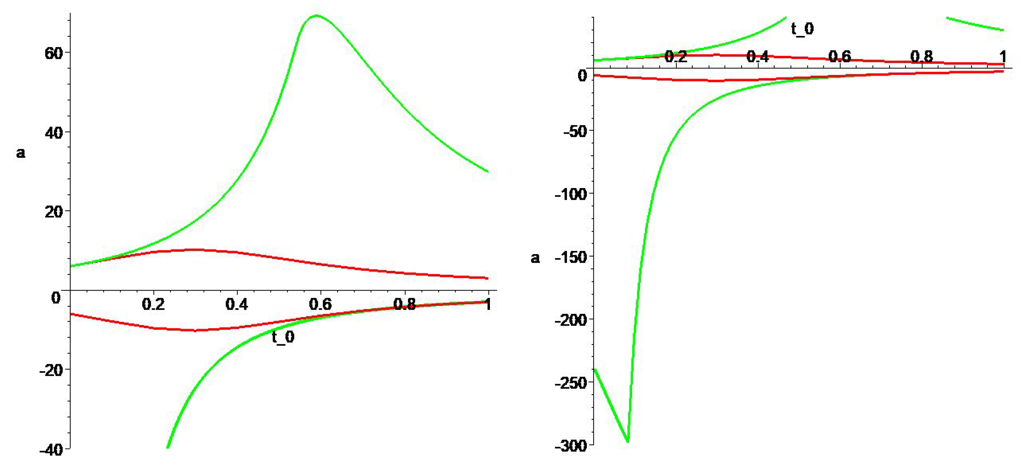
This solvability condition will be significantly improved by the following condition (33). Condition (32) coincides with condition (33) only in two cases (when the coefficient $p\left(t\right)$ is non-negative, that is, for $t_0=0$, $a>0$ and for $t_0=1$, $a<$0 (see Figure 1)). In other cases, condition (33) is much weaker, than (32), moreover, the constants in (33) are unimprovable.

Figure 1. The graphs of the functions −$A^{-}$ and $A^{+}$ (33) are indicated in green, the solvability bounds (32) obtained using the Banach’s principle are indicated in red.

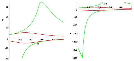
Direct verification of the conditions of Theorem 1 makes it possible to obtain necessary and sufficient conditions for the constants $t_0$ and a under which inequality (10) is satisfied for all $0⩽t_3⩽t_1⩽1$. We find that for such $p^{+}$, $p^{-}$ by Theorem 1 problem (1) and (2) enjoys the property ${\mathcal{A}}_1$ if and only if

$$-A^{-}\left(t_0\right)<a<A^{+}\left(t_0\right),$$

(33)

where the functions $A^{-}$, $A^{+}$ are defined by equalities (see Figure 1)

$$A^{+}\left(t_0\right)=\left\{\begin{array}{c}6/{(1-t_0)}^3\mathrm{for}{t}_0\in [0,t^{*}],\hfill \\ \underset{0<t_3⩽t_1<t_0}{min}\frac{3(q_1+\sqrt{q_1^2+4q_2})}{q_2}\mathrm{for}{t}_0\in (t^{*},1],\hfill \end{array}\right.$$

$t^{*}$ is a unique real solution of the equation ${(3t_0-1)}^2/4={(1-t_0)}^3$ ($t^{*}\approx 0.54$),

$$\begin{array}{cc}\hfill & q_1={(t_0-t_1)}^3-3(1-t_1){(t_0-t_3)}^2+3t_0-1,\hfill \\ \hfill & q_2=t_1^2(3-t_0-2t_3){(t_0-t_3)}^2(3t_0-t_1)-(3t_0-1){(t_1-t_3)}^2(3t_0-t_1-2t_3);\hfill \end{array}$$

$$A^{-}\left(t_0\right)=\left\{\begin{array}{c}\underset{t_0<t_3⩽t_1<1}{min}\left\{\frac{3(r_1-\sqrt{r_1^2-4r_2})}{r_2},\frac{6}{t_0^2(3-t_0)}\right\}\mathrm{for}{t}_0\in [0,t_{*}),\hfill \\ \frac{6}{t_0^2(3-t_0)}\mathrm{for}{t}_0\in [t_{*},1],\hfill \end{array}\right.$$

$t_{*}$ is a unique solution of the equation $t_0^2(3-t_0)=2-3t_0$ ($t_{*}\approx 0.47$),

$$\begin{array}{cc}\hfill & r_1=(t_1^2(3t_0-t_1)+3{(t_0-t_3)}^2(t_1-1))/6,\hfill \\ \hfill & r_2=(t_1(t_0+2t_3)(3t_0-t_1)+(3t_1-t_0-2t_3)(1+t_1-3t_0)){(t_0-t_3)}^2(t_1-1)/36.\hfill \end{array}$$

If the parameter a satisfies the inequality (33), then Cauchy problem (31) is uniquely solvable for all measurable deviations of the argument $h:[0,1]\to [0,1]$. If the condition (33) is not satisfied, then there is a measurable function $h:[0,1]\to [0,1]$ such that Cauchy problem (31) is not uniquely solvable.

It follows that, for $t_0\in [1/5,t^{*}]$, problem (1) and (2) possesses property ${\mathcal{A}}_1$ if and only if

$$a\in \left(-\frac{6}{t_0^2(3-t_0)},\frac{6}{{(1-t_0)}^3}\right).$$

In particular, if $t_0=1/2$, then the inequality $-\frac{48}{5}<a<48$ is necessary and sufficient for problem (1) and (2) to enjoy property ${\mathcal{A}}_1$. Thus, for $b\in \mathbf{L}[0,1]$ the Cauchy problem

$$\left\{\begin{array}{c}\ddot{x}\left(t\right)=b\left(t\right)(t-1/2)x\left(h\left(t\right)\right)+f\left(t\right),t\in [0,1],\hfill \\ x\left(0\right)=c_0,\dot{x}\left(0\right)=c_1,\hfill \end{array}\right.$$

(34)

is uniquely solvable for all measurable $h:[0,1]\to [0,1]$ if

$$0⩽b\left(t\right)⩽48,b\left(t\right)\not\equiv 48,$$

or

$$-48/5⩽b\left(t\right)⩽0,b\left(t\right)\not\equiv -48/5,$$

and the constants 48 and $48/5$ cannot be increased.

Let us apply Theorem 2 to the Cauchy problem

$$\left\{\begin{array}{c}\ddot{x}\left(t\right)=b\left(t\right)(t-1/2)x\left(h\left(t\right)\right)-d\left(t\right)x\left(g\left(t\right)\right)+f\left(t\right),t\in [0,1],\hfill \\ x\left(0\right)=c_0,\dot{x}\left(0\right)=c_1,\hfill \end{array}\right.$$

(35)

where $b\left(t\right)=0$ for $t\in [0,1/2]$, $b\left(t\right)⩾0$ for $t\in (1/2,1]$, $d\left(t\right)⩾0$ for all $t\in [0,1]$. So, here we have not changed the operator $T^{+}$ from Cauchy problem (34), but consider an arbitrary operator $T^{-}$. Application of Theorem 2 gives the following solvability condition: the Cauchy problem (35) is uniquely solvable for all measurable functions h, $g:[0,1]\to [0,1]$ if $\underset{t\in [1/2,1]}{sup}b\left(t\right)⩽48$, $b\left(t\right)\not\equiv 48$ for $t\in [1/2,1]$, and

$${\int }_0^{1}d\left(t\right)dt⩽4+4\sqrt{1-\frac{\underset{t\in [1/2,1]}{sup}b\left(t\right)}{48}}.$$

For $\underset{t\in [1/2,1]}{sup}b\left(t\right)=48$, we have the solvability condition ${\int }_0^{1}d\left(t\right)dt⩽4$, which is expected to be significantly less than $48{\int }_0^{1/2}(1/2-s)ds=6$ from the solvability conditions of problem (34). This is explained by the fact that when considering problem (35) we imposed not pointwise restrictions on the operator $T^{-}$, but weaker integral restrictions. All constants in these solvability conditions cannot be increased.

7. Discussion

In this paper we have presented a new class of sufficient conditions for the unique solvability of the Cauchy problem for linear functional differential equations. These conditions are necessary conditions for the unique solvability of the Cauchy problem for all equations from a certain family. We use a new kind of family, when we impose different restrictions on linear operators in functional differential equation.

The obtained solvability conditions improve all known ones. They are unimprovable in the sense that if they are not satisfied, then in the considered family of equations given by relations (3)–(6), there exists an equation for which the Cauchy problem is not uniquely solvable.

We consider only linear functional differential equations, but generalizations to non-linear equations with Lipschitz nonlinearities are possible and do not encounter fundamental difficulties. Natural generalizations of the results obtained to other boundary value problems and functional differential equations with continuous and discrete time are also possible. Moreover, the obtained results can be extended to fractional differential equations (see, for example, [36], where a method close to ours and to the method of the books [1,5] was used). The proposed methodology in the paper can be used for real problems (such as described in [37]).

References

- Azbelev, N.V.; Maksimov, V.P.; Rakhmatullina, L.F. Introduction to the Theory of Functional Differential Equations: Methods and Applications; Hindawi Publishing Corporation: New York, NY, USA; Cairo, Egypt, 2007; ISBN 978-9775945495. [Google Scholar]
- Agarwal, R.P.; Berezansky, L.; Braverman, E.; Domoshnitsky, A. Nonoscillation Theory of Functional Differential Equations with Applications; Springer Science & Business Media: Berlin/Heidelberg, Germany, 2012; ISBN 978-146143455-9/1461434548/978-146143454-2. [Google Scholar] [CrossRef]
- Azbelev, N.V.; Maksimov, V.P.; Rakhmatullina, V.P. Introduction to the Theory of Functional Differential Equations; Nauka: Moscow, Russia, 1991. (In Russian) [Google Scholar]
- Azbelev, V.P. Contemporary theory of functional differential equations and some classic problems. Nonlinear Anal. Theory Methods Appl. 2005, 63, e2603–e2605. [Google Scholar] [CrossRef]
- Azbelev, N.V.; Rakhmatullina, L.F. Theory of linear abstract functional-differential equations and applications. Mem. Differ. Equ. Math. Phys. 1996, 8, 1–102. [Google Scholar]
- Beklaryan, L.A.; Beklaryan, A.L. Solvability problems for a linear homogeneous functional-differential equation of the pointwise type. Differ. Equ. 2017, 2, 145–156. [Google Scholar] [CrossRef]
- Belkina, T.A.; Konyukhova, N.B.; Kurochkin, S.V. Singular initial-value and boundary-value problems for integrodifferential equations in dynamical insurance models with investments. J. Math. Sci. 2016, 218, 571–585. [Google Scholar] [CrossRef]
- Byszewski, E.I.; Akca, H. Existence of solutions of a semilinear functional-differential evolution nonlocal problem. Nonlinear Anal. Theory Methods Appl. 1998, 34, 65–72. [Google Scholar] [CrossRef]
- Myshkis, A.D. Mixed Functional Differential Equations. J. Math. Sci. 2005, 129, 4111–4226. [Google Scholar] [CrossRef]
- Šremr, J. On the Cauchy type problem for two-dimensional functional differential systems. Mem. Differ. Equ. Math. Phys. 2007, 40, 77–134. [Google Scholar]
- Agarwal, R.P. Boundary Value Problems from Higher Order Differential Equations; World Scientific: Singapore, 1986; ISBN 978-981-4513-63-0. [Google Scholar] [CrossRef]
- Corduneanu, C.; Li, Y.; Mahdavi, M. Functional Differential Equations. Advances and Applications; John Wiley & Sons: Hoboken, NJ, USA, 2016; ISBN 978-1119189473. [Google Scholar] [CrossRef]
- Hale, J.K. Theory of Functional Differential Equations; Springer: New York, NY, USA, 1977; ISBN 978-1-4612-9892-2/978-1-4612-9894-6. [Google Scholar] [CrossRef]
- Hale, J.K.; Lunel, S.M.V. Introduction to Functional Differential Equations; Springer Science & Business Media: Berlin/Heidelberg, Germany, 2013; ISBN 978-0-387-94076-2/978-1-4612-4342-7. [Google Scholar] [CrossRef]
- Henderson, J.; Luca, R. Boundary Value Problems for Systems of Differential, Difference and Fractional Equations. Positive Solutions; Elsevier: Amsterdam, The Netherlands, 2015; ISBN 9780128036525/9780128036792. [Google Scholar]
- Lomtatidze, A.; Mukhigulashvili, S. On periodic solutions of second order functional differential equations. Mem. Differ. Equ. Math. Phys. 1995, 5, 125–126. [Google Scholar]
- Lomtatidze, A.; Mukhigulashvili, S. On a two-point boundary value problem for second-order functional-differential equations, i. Mem. Differ. Equ. Math. Phys. 1997, 10, 125–128. [Google Scholar]
- Lomtatidze, A.; Mukhigulashvili, S. On a two-point boundary value problem for second-order functional-differential equations, ii. Mem. Differ. Equ. Math. Phys. 1997, 10, 150–152. [Google Scholar]
- Hakl, R.; Lomtatidze, A. On the Cauchy problem for first order linear differential equations with a deviating argument. Arch. Math. 2002, 38, 61–71. [Google Scholar]
- Hakl, R.; Lomtatidze, A.; Půža, B. New optimal conditions for unique solvability of the Cauchy problem for first order linear functional differential equations. Math. Bohem. 2002, 127, 509–524. [Google Scholar] [CrossRef]
- Bravyi, E.; Hakl, R.; Lomtatidze, A. Optimal conditions for unique solvability of the Cauchy problem for first order linear functional differential equations. Czech. Math. J. 2002, 52, 513–530. [Google Scholar] [CrossRef]
- Šremr, J. Solvability conditions of the Cauchy problem for two-dimensional systems of linear functional differential equations with monotone operators. Math. Bohem. 2007, 132, 263–295. [Google Scholar] [CrossRef]
- Šemr, J.; Hakl, R. On the Cauchy problem for two-dimensional systems of linear functional differential equations with monotone operators. Nonlinear Oscil. 2004, 10, 569–582. [Google Scholar] [CrossRef]
- Hakl, R.; Lomtatidze, A.; Půža, B. On periodic solutions of first order linear functional differential equations. Nonlinear Anal. Theory Methods Appl. 2002, 49, 929–945. [Google Scholar] [CrossRef]
- Hakl, R.; Lomtatidze, A.; Šremr, J. On an antiperiodic type boundary value problem for first order linear functional differential equations. Arch. Math. 2002, 38, 149–160. [Google Scholar]
- Bravyi, E.I. Solvability of the periodic problem for higher-order linear functional differential equations. Differ. Equ. 2015, 5, 571–585. [Google Scholar] [CrossRef]
- Bravyi, E. On solvability conditions for the Cauchy problem for second order functional differential equations with non-Volterra operators and composite pointwise restrictions. Mem. Differ. Equ. Math. Phys. 2022, 87, 37–52. [Google Scholar]
- Bravyi, E.I. Solvability of the Cauchy problem for higher-order linear functional differential equations. Differ. Equ. 2012, 48, 465–476. [Google Scholar] [CrossRef]
- Dilnaya, N.Z.; Ronto, A.N. Some new conditions for the solvability of the Cauchy problem for systems of linear functional-differential equations. Ukr. Math. J. 2004, 56, 1033–1053. [Google Scholar] [CrossRef]
- Bravyi, E. On the solvability of the Cauchy problem for functional differential equations with mixed restrictions on functional operators. Funct. Differ. Equ. 2023, 1–2, 21–38. [Google Scholar]
- Kantorovich, L.V.; Akilov, G.P. Functional Analysis; Pergamon Press, 1982; ISBN 978-0-08-023036-8. [Google Scholar] [CrossRef]
- Krein, S.G. Linear Equations in Banach Spaces; Birkhäuser: Boston, MA, USA, 1982; ISBN 978-0-8176-3101-7/978-1-4684-8068-9. [Google Scholar] [CrossRef]
- Kantorovich, L.V. Descriptive Theory of Sets and Functions. Functional Analysis in Semi-Ordered Spaces; CRC Press: Boca Raton, FL, USA, 1996; ISBN 9782884490122. [Google Scholar]
- Wang, W.; Zhang, H.; Jiang, X.; Yang, X. A high-order and efficient numerical technique for the nonlocal neutron diffusion equation representing neutron transport in a nuclear reactor. Ann. Nucl. Energy 2024, 195, 110163. [Google Scholar] [CrossRef]
- Yang, X.; Zhang, Q.; Yuan, G.; Sheng, Z. On positivity preservation in nonlinear finite volume method for multi-term fractional subdiffusion equation on polygonal meshes. Nonlinear Dyn. 2018, 92, 595–612. [Google Scholar] [CrossRef]
- Bohner, M.; Domoshnitsky, A.; Padhi, S.; Srivastava, S.N. Vallée-Poussin theorem for equations with Caputo fractional derivative. Math. Slovaca 2023, 73, 713–728. [Google Scholar] [CrossRef]
- Zhang, H.; Liu, Y.; Yang, X. An efficient ADI difference scheme for the nonlocal evolution problem in three-dimensional space. J. Appl. Math. Comput. 2023, 69, 651–674. [Google Scholar] [CrossRef]
Disclaimer/Publisher’s Note: The statements, opinions and data contained in all publications are solely those of the individual author(s) and contributor(s) and not of MDPI and/or the editor(s). MDPI and/or the editor(s) disclaim responsibility for any injury to people or property resulting from any ideas, methods, instructions or products referred to in the content. |
© 2023 by the author. Licensee MDPI, Basel, Switzerland. This article is an open access article distributed under the terms and conditions of the Creative Commons Attribution (CC BY) license (https://creativecommons.org/licenses/by/4.0/).