Efficient Automatic Subdifferentiation for Programs with Linear Branches

Abstract

Computing an element of the Clarke subdifferential of a function represented by a program is an important problem in modern non-smooth optimization. Existing algorithms either are computationally inefficient in the sense that the computational cost depends on the input dimension or can only cover simple programs such as polynomial functions with branches. In this work, we show that a generalization of the latter algorithm can efficiently compute an element of the Clarke subdifferential for programs consisting of analytic functions and linear branches, which can represent various non-smooth functions such as max, absolute values, and piecewise analytic functions with linear boundaries, as well as any program consisting of these functions such as neural networks with non-smooth activation functions. Our algorithm first finds a sequence of branches used for computing the function value at a random perturbation of the input; then, it returns an element of the Clarke subdifferential by running the backward pass of the reverse-mode automatic differentiation following those branches. The computational cost of our algorithm is at most that of the function evaluation multiplied by some constant independent of the input dimension n, if a program consists of piecewise analytic functions defined by linear branches, whose arities and maximum depths of branches are independent of n.

1. Introduction

Automatic differentiation refers to various techniques to compute the derivatives of a function represented by a program, based on the well-known chain rule of calculus. It has been widely used across various domains, and diverse practical automatic differentiation systems have been developed [1,2,3]. In particular, reverse-mode automatic differentiation [4] has been a driving force of the rapid advances in numerical optimization [5,6,7].

There are two important properties of reverse-mode automatic differentiation: correctness and efficiency. For programs consisting of smooth functions, it is well known that reverse-mode automatic differentiation always computes the correct derivatives [8,9]. Furthermore, for programs returning a scalar value, it efficiently computes their derivatives in the sense that its computational cost is at most proportional to that of the function evaluation, where the additional multiplicative factor is bounded by five for rational functions [10,11] and by some constant that depends on the underlying implementation of smooth functions; if the arities of the functions are independent of the input dimension n, then this constant is also independent of n [12]. Such correctness and efficiency of reverse-mode automatic differentiation, referred to as the Cheap Gradient Principle, have been of central importance for modern nonlinear optimization algorithms [13].

In practical problems, a program often involves branches (e.g., max and an absolute value), and the corresponding target function can be non-smooth. In other words, the derivative of the program may not exist at some inputs. In this work, we investigated a Cheap Subgradient Principle: an efficient algorithm that correctly computes an element of the Clarke subdifferential, a generalized notion of the derivative, for scalar programs. One naïve approach is to directly apply reverse-mode automatic differentiation to the Clarke subdifferential. Such a method is computationally cheap as in the smooth case; however, due to the absence of the sharp chain rule for the Clarke subdifferential, it is incorrect in general even if the target function is differentiable [8,14,15].

There have been extensive research efforts to correctly compute an element of the Clarke subdifferential. A notable line of work is based on the lexicographic subdifferential [16], which is a subset of the Clarke subdifferential, but a sharp chain rule holds under some structural assumptions. Based on this, a series of works [17,18,19,20] has shown that an element of the lexicographic subdifferential can be computed by evaluating n directional derivatives, where n denotes the input dimension. Nevertheless, since this approach requires computing n directional derivatives, it incurs a multiplicative factor n in its computational cost compared to that of function evaluation in the worst case.

To avoid such an input-dimension-dependent factor, a two-step randomized algorithm for programs with branches has been proposed [14]. In the first step, the algorithm chooses a random direction $\delta$ and finds a sequence of branch selections based on the directional derivative with respect to $\delta$ under some qualification condition [14,21]. Then, the second step computes the derivative corresponding to the branches returned in the first step, which is shown to be an element of the Clarke subdifferential. Here, the second step can also be efficiently implemented via reverse-mode automatic differentiation. As a result, this two-step algorithm correctly computes an element of the Clarke subdifferential under the qualification condition, with the computational cost independent of the input dimension. However, this result is only for piecewise polynomial programs, defined by branches and finite compositions of monomials and affine functions.

In this work, we propose an efficient automatic subdifferentiation algorithm by generalizing the algorithm in [14] described above. Our algorithm correctly computes an element of the Clarke subdifferential for programs consisting of any analytic functions (including polynomials) and linear branches. As in the prior efficient automatic (sub)differentiation works, the computational cost of our algorithm is that of the function evaluation multiplied by some constant independent of the input dimension n, if a program consists of piecewise analytic functions (defined by linear branches) whose arities and maximum depths of branches are independent of n (e.g., max and the absolute value).

Related Works

Non-smooth optimization: Although smooth functions are easy to formulate and optimize, they have limited applicability as non-smoothness appears in various science and engineering problems. For example, real-world problems in thermodynamics often involve discrete switching between thermodynamic phases, which can be modeled by non-smooth functions. Dynamic simulation and optimization under these models often require the treatment of these models [22,23]. In machine learning applications, hinge loss, ReLU$\left(x\right)=max\{x,0\}$, and maxpool operations are often used, which makes the optimization objective non-smooth [6,24,25]. For optimizing convex, but non-smooth functions, subderivative methods are widely used for approximating a local minimum [26,27]. However, for non-convex functions, the subderivative does not exist in general, and researchers have investigated the generalized notion of derivatives (e.g., the Clarke subdifferential).

Optimization algorithms using generalized derivatives: Recently, the convergence properties of optimization algorithms based on generalized derivatives for non-convex and non-smooth functions have received much attention. Ref. [28] proved that, for locally Lipschitz functions, the stochastic gradient method, where the gradient is chosen from the Clarke subdifferential, converges to a stationary point. However, as we introduced in the previous section, computing an element of the Clarke subdifferential is computationally expensive or can be efficient only for a specific class of programs. Ref. [29] proposed a new notion of gradient called the conservative gradient, which can be efficiently computed; nevertheless, its convergence property is not well understood, especially under practical setups.

2. Problem Setup

2.1. Notations

For $n\in \mathbb{N}\cup \left\{0\right\}$, we denote $\left[n\right]\triangleq \{1,\cdots ,n\}$, where $\left[0\right]=\varnothing$. For any set $\mathcal{S}$, we use ${\mathcal{S}}^0\triangleq \left\{\left(\right)\right\}$, where $\left(\right)$ denotes the zero-dimensional vector. For any vector $x\in {\mathcal{S}}^n$ and $i\in \left[n\right]$, we denote $x_i$ for the i-th coordinate of x and $x_{:i}\triangleq (x_1,\cdots ,x_{i-1})$, where $x_{:1}=\left(\right)$; similarly, for any $x\in {\mathcal{S}}^n$ and index set $\mathcal{I}=\{i_1,\cdots ,i_k\}\subseteq \left[n\right]$ with $i_1<\cdots <i_k$, we use $x_{\mathcal{I}}\triangleq (x_{i_1},\cdots ,x_{i_k})$. For any $u=(u_1,\cdots ,u_n)\in {\mathbb{R}}^n$ and $v=(v_1,\cdots ,v_m)\in {\mathbb{R}}^m$, we use $u\oplus v\triangleq (u_1,\cdots ,u_n,v_1,\cdots ,v_m)$; when $n=m$, we write $⟨u,v⟩$ to denote the standard inner product between u and v. For any $x\in \mathbb{R}$, sign$\left(x\right)=1$ if $x>0$ and sign$\left(x\right)=-1$ otherwise. For any real-valued vector x, len$\left(x\right)$ denotes the length of x, i.e., len$\left(x\right)=n$ if $x\in {\mathbb{R}}^n$. For any set $\mathcal{S}\subseteq {\mathbb{R}}^n$, we use cl$\left(\mathcal{S}\right)$, int$\left(\mathcal{S}\right)$, and conv$\left(\mathcal{S}\right)$ to denote the closure, interior, and convex hull of $\mathcal{S}$, respectively. We lastly define the Clarke subdifferential. Given a function $f:{\mathbb{R}}^n\to \mathbb{R}$ and the set $\mathcal{D}\subseteq {\mathbb{R}}^n$ of all points at which f is differentiable, the Clarke subdifferential of f at $x\in {\mathbb{R}}^n$ is a set defined as

$$\begin{array}{c}\hfill {\partial }^{c}f\left(x\right)\triangleq \mathrm{conv}\left\{s\in {\mathbb{R}}^n:\exists {\left\{u_t\right\}}_{t\in \mathbb{N}}\subseteq \mathcal{D}\mathrm{such}\mathrm{that}{u}_t\to x\mathrm{and}\nabla f\left(u_t\right)\to s\right\}.\end{array}$$

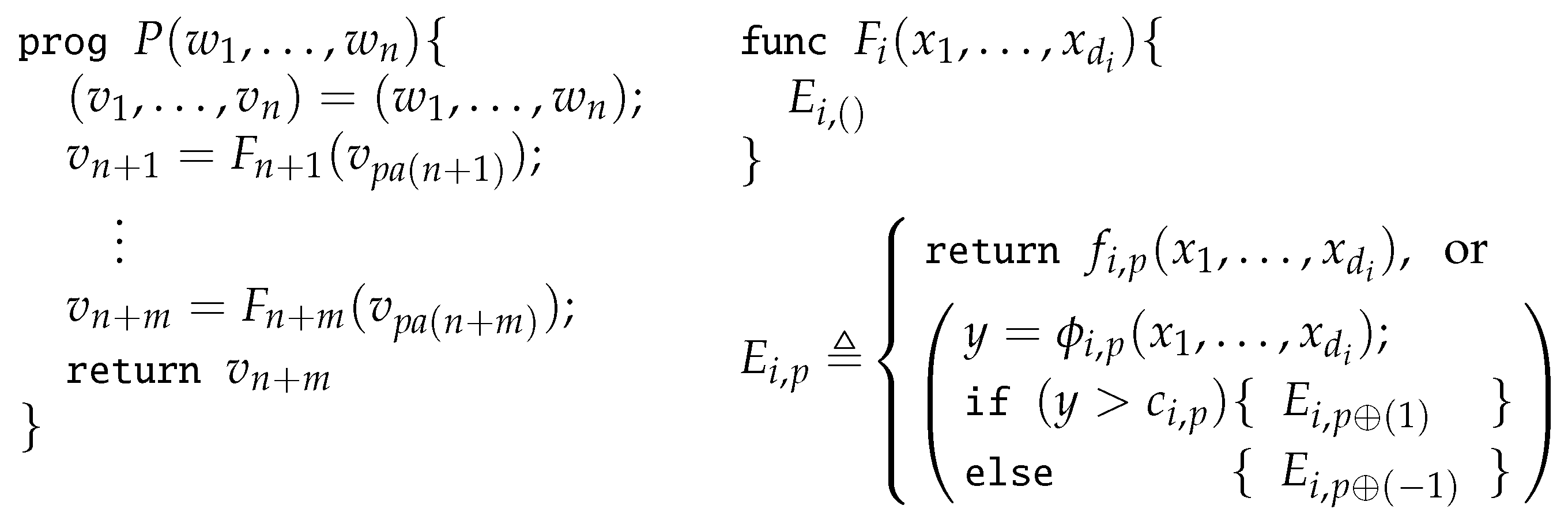
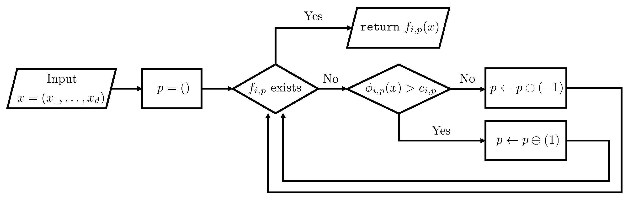
2.2. Programs with Branches

We considered a program P defined in Figure 1 (left). P applies a series of primitive functions $F_{n+1},\cdots ,F_{n+m}$ to compute intermediate variables $v_{n+1},\cdots ,v_{n+m}$ and, then, returns the last result $v_{n+m}$. Each primitive function $F_i:{\mathbb{R}}^{d_i}\to \mathbb{R}$ is continuous and defined in an inductive way as in Figure 1 (right): $F_i$ either applies a function $f_{i,\left(\right)}$ or branches via (possibly nested) if–else statements. Namely, $F_i$ is a continuous, piecewise function. If $F_i$ branches with an input $(x_1,\cdots ,x_{d_i})$, then it first evaluates $y={\varphi }_{i,\left(\right)}(x_1,\cdots ,x_{d_i})$ for some ${\varphi }_{i,\left(\right)}:{\mathbb{R}}^{d_i}\to \mathbb{R}$ and checks whether $y>c_{i,\left(\right)}$ or not for some threshold value $c_{i,\left(\right)}\in \mathbb{R}$. If $y>c_{i,\left(\right)}$, it executes a code $E_{i,\left(1\right)}$ that either applies a function $f_{i,\left(1\right)}$ or executes another code $E_{i,(1,1)}$ or $E_{i,(1,-1)}$ depending on whether ${\varphi }_{i,\left(1\right)}(x_1,\cdots ,x_{d_i})>c_{i,\left(1\right)}$ or not. The case $y\le c_{i,\left(\right)}$ is handled in a similar way. Here, we assumed that each $F_i$ has finitely many branches. In short, each primitive function $F_i$ first finds a proper piece labeled by $p\in {\bigcup }_{j=0}^{\infty }{\{-1,1\}}^j$ and, then, returns $f_{i,p}(x_1,\cdots ,x_{d_i})$. We illustrate a flow chart for a primitive function $F_i$ in Figure 2.

Figure 1. Definitions of a program P (left) and primitive functions $F_{n+1},\cdots ,F_{n+m}$ (right).

Figure 2. A flow chart illustrating a primitive function $F_i$.

We present an example code for a primitive function $F_i$ that returns $max\{x_1,x_2,x_3\}$ in Figure 3. In this example, $F_i$ branches at most twice: its first branch is determined by ${\varphi }_{i,\left(\right)}(x_1,x_2,x_3)=x_1-x_2$, which is stored in y in the second line in Figure 3. If $y>0$ (the third line with $c_{i,\left(\right)}=0$), then it executes $E_{1,\left(1\right)}$, which corresponds to lines 4–6. Otherwise, it moves to $E_{1,(-1)}$, which corresponds to the lines 8–10. Suppose $E_{1,\left(1\right)}$ is executed (i.e., $y>0$ in line 3). Then, it computes ${\varphi }_{i,\left(1\right)}(x_1,x_2,x_3)=x_1-x_3$ and stores it in y as in line 4. If $y>0$, then $E_{i,(1,1)}$ is executed, which returns the value of $x_1$ (i.e., $f_{i,(1,1)}(x_1,x_2,x_3)=x_1$). Otherwise, $E_{i,(1,-1)}$ is executed, which returns the value of $x_3$ (i.e., $f_{i,(1,-1)}(x_1,x_2,x_3)=x_3$).

Figure 3. Example code for the max function $F_i:(x_1,x_2,x_3)\mapsto max\{x_1,x_2,x_3\}$.

We considered each $v_i$ and $v_{pa\left(i\right)}$ as a function of an input $w\in {\mathbb{R}}^n$. Specifically, for all $i\in \left[n\right]$, we use $v_i\left(w\right)\triangleq w_i$; and for all $i\in [n+m]\setminus \left[n\right]$, we use $v_i\left(w\right)\triangleq F_i\left(v_{\left(i\right)}\left(w\right)\right)$ and $v_{pa\left(i\right)}\left(w\right)\triangleq (v_{j_1}\left(w\right),\cdots ,v_{j_{d_i}}\left(w\right))$, where $pa\left(i\right)=\{j_1,\cdots ,j_{d_i}\}$ with $0<j_1<\cdots <j_{d_i}<i$. Under this notation, $w\mapsto v_{n+m}\left(w\right)$ denotes the target function represented by the program P. We often omit w and write $v_i$ and $v_{pa\left(i\right)}$ if it is clear from the context. We denote the gradient (or Jacobian) of functions with respect to an input w by the operator: e.g., D$v_i\left(w\right)\triangleq \partial v_i\left(w\right)/\partial w$ and D${\varphi }_{i,p}\left(v_{pa\left(i\right)}\left(w\right)\right)\triangleq \partial {\varphi }_{i,p}\left(v_{pa\left(i\right)}\left(w\right)\right)/\partial w$.

Throughout this paper, we focus on programs with linear branches; that is, each ${\varphi }_{i,p}(x_1,\cdots ,x_d)$ is linear in $x_1,\cdots ,x_d$. Primitive functions with linear branches can express fundamental non-smooth functions such as max, the absolute value, bilinear interpolation, and any piecewise analytic functions with finite linear boundaries. They have been widely used in various fields including machine learning, electrical engineering, and non-smooth analysis. For example, max–min representation (or the abs–normal form) has been extensively studied in non-smooth analysis [30,31]. Furthermore, neural networks using the ReLU$\left(x\right)=max\{x,0\}$ activation function and maxpool operations are widely used in machine learning, computer vision, load forecasting, etc. [6,24,25]. The assumption on linear branches will be formally introduced in Assumption 1 in Section 3.1.

2.3. Pieces of Programs

We introduce useful notations here. For each $i\in [n+m]\setminus \left[n\right]$, we define the set of the pieces of $F_i$ as

$$\begin{array}{c}\hfill {\mathsf{\Gamma }}_i\triangleq \left\{p\in \bigcup _{j=0}^{\infty }{\{-1,1\}}^j:E_{i,p}=\mathrm{return}{f}_{i,p}(x_1,\cdots ,x_{d_i})\right\}.\end{array}$$

We also define $\mathsf{\Gamma }\triangleq {\left\{\left(\right)\right\}}^n\times {\prod }_{i=n+1}^m{\mathsf{\Gamma }}_i$ for the pieces of the overall program. Here, we include an auxiliary piece $\left(\right)$ for the first n indices so that ${\gamma }_i\in {\mathsf{\Gamma }}_i$ for any $\gamma =({\gamma }_1,\cdots ,{\gamma }_{n+m})\in \mathsf{\Gamma }$ and $i\in [n+m]\setminus \left[n\right]$. For each $i\in [n+m]\setminus \left[n\right]$, we define the set of the inputs to $F_i$ that corresponds to the piece $p\in {\mathsf{\Gamma }}_i$, as 

$$\begin{array}{c}\hfill {\mathcal{X}}_{i,p}\triangleq \{x\in {\mathbb{R}}^{d_i}:F_i\mathrm{selects}{f}_{i,p}\mathrm{at}\mathrm{the}\mathrm{input}x\}.\end{array}$$

Then, $\{{\mathcal{X}}_{i,p}:p\in {\mathsf{\Gamma }}_i\}$ forms a partition of ${\mathbb{R}}^{d_i}$. Likewise, we also define the set of the inputs to the overall program P that corresponds to $\gamma \in \mathsf{\Gamma }$, as 

$$\begin{array}{c}\hfill {\mathcal{W}}_{\gamma }\triangleq \{w\in {\mathbb{R}}^n:v_{pa\left(i\right)}\left(w\right)\in {\mathcal{X}}_{i,{\gamma }_i}\mathrm{for}\mathrm{all}i\in [n+m]\setminus \left[n\right]\}.\end{array}$$

Then, $\{{\mathcal{W}}_{\gamma }:\gamma \in \mathsf{\Gamma }\}$ forms a partition of ${\mathbb{R}}^n$. Lastly, for each $\gamma \in \mathsf{\Gamma }$, we inductively define the function $v_{i,\gamma }:{\mathbb{R}}^n\to \mathbb{R}$ that corresponds to $v_i(·)$, but is obtained by using the ${\gamma }_j$ piece of each $F_j$, as 

$$\begin{array}{c}\hfill v_{i,\gamma }\left(w\right)\triangleq \left\{\begin{array}{cc}{w}_i\hfill & \mathrm{if}i\in \left[n\right]\hfill \\ f_{i,{\gamma }_i}\left(v_{pa\left(i\right),\gamma }\left(w\right)\right)\hfill & \mathrm{if}i\in [n+m]\setminus \left[n\right],\hfill \end{array}\right.\end{array}$$

where $v_{\left(i\right),\gamma }(·)$ is defined as in $v_{\left(i\right)}(·)$. Then, $v_{i,\gamma }(·)$ coincides with $v_i(·)$ on ${\mathcal{W}}_{\gamma }$ for all $i\in [n+m]$.

2.4. Reverse-Mode Automatic Differentiation

Reverse-mode automatic differentiation is an algorithm for computing the gradient $v_{n+m}\left(w\right)$ of the target function (if it exists) by sequentially running one forward pass (Algorithm 1) and one backward pass (Algorithm 2). Given $w\in {\mathbb{R}}^n$, its forward pass computes $v_{n+1}\left(w\right),\cdots ,v_{n+m}\left(w\right)$ and corresponding pieces ${\gamma }_i\in {\mathsf{\Gamma }}_i$ such that $w\in {\mathcal{W}}_{\gamma }$ for $\gamma =(\left(\right),\cdots ,\left(\right),{\gamma }_{n+1},\cdots ,{\gamma }_{n+m})$. Namely, we have $v_i\left(w\right)=v_{i,\gamma }\left(w\right)$ for all $i\in [n+m]$.

Algorithm 1 Forward pass of reverse-mode automatic differentiation

1: Input: P, $(w_1,\cdots ,w_n)$ 2: Initialize: $(v_1,\dots ,v_n)=(w_1,\dots ,w_n)$ 3: for $i=n+1,\dots ,n+m$ do 4:    Let $p=\left(\right)$ 5:    while  $p\notin {\mathsf{\Gamma }}_i$  do 6:      $p=p\oplus \left((\mathrm{sign}{\varphi }_{i,p}\left(v_{pa\left(i\right)}\right)-c_{i,p})\right)$ 7:     end  while 8:    Set ${\gamma }_i=p$ and $v_i=f_{i,{\gamma }_i}\left(v_{pa\left(i\right)}\right)$ 9: end  for 10: return  $(v_1,\dots ,v_{n+m})$, $({\gamma }_{n+1},\dots ,{\gamma }_{n+m})$

Algorithm 2 Backward pass of reverse-mode automatic differentiation

1: Input:  P, $(v_1,\dots ,v_{n+m})$, $({\gamma }_{n+1},\dots ,{\gamma }_{n+m})$ 2: Initialize:  $(g{v}_1,\cdots ,g{v}_{n+m})=(0,\cdots ,0,1)$ 3: for  $i=n+m,\dots ,n+1$  do 4:     for  $j\in \left(i\right)$  do 5:      ${\displaystyle g{v}_j=g{v}_j+g{v}_i·\frac{\partial f_{i,{\gamma }_i}}{\partial v_j}\left(v_{\left(i\right)}\right)}$ 6:     end  for 7: end  for 8: return  $(g{v}_1,\dots ,g{v}_n)$

Given $v_1\left(w\right),\cdots ,v_{n+m}\left(w\right)$ and $\gamma$, the backward pass computes ${Dv}_{n+m,\gamma }\left(w\right)$ by applying the chain rule to the composition of differentiable functions $f_{n+1,{\gamma }_{n+1}},\cdots ,f_{n+m,{\gamma }_{n+m}}$. In particular, it iteratively updates $g{v}_i$ and returns $(g{v}_1,\cdots ,g{v}_n)={Dv}_{n+m,\gamma }\left(w\right)$. It is well known that reverse-mode automatic differentiation computes the correct gradient, i.e., $g{v}_i$ coincides with $\partial v_{n+m}\left(w\right)/\partial w_i$ for all $i\in \left[n\right]$, if primitive functions $F_{n+1},\cdots ,F_{n+m}$ do not have any branches [8,9]. However, if some $F_i$ uses branches, it may return arbitrary values even if the target function $v_{n+m}(·)$ is differentiable at w [14,32,33]. In the rest of the paper, we use AD to denote reverse-mode automatic differentiation.

Our algorithm computing an element of the Clarke subdifferential is similar to AD: it first finds some pieces ${\gamma }_i^{*}\in {\mathsf{\Gamma }}_i$ and applies the backward pass of AD (Algorithm 2) to compute its output. Here, we chose the pieces ${\gamma }_i^{*}$ that are used for computing the forward pass with some perturbed input, not the original one. Hence, our pieces and that of AD are different in general, which enables our algorithm to correctly compute an element of the Clarke subdifferential. We provide more details including the intuition behind our algorithm in Section 3.2 and Section 3.3.

3. Efficient Automatic Subdifferentiation

In this section, we present our algorithm for efficiently computing an element of the Clarke subdifferential. To this end, we first introduce a class of primitive functions, which we consider in the rest of this paper. Then, we describe our algorithm after illustrating its underlying intuition via an example. Lastly, we analyze the computational complexity of our algorithm.

3.1. Assumptions on Primitive Functions

We considered primitive functions that satisfy the following assumptions.

Assumption 1. 

For any $i\in [n+m]\setminus \left[n\right]$, $p\in {\mathsf{\Gamma }}_i$, and $j\in \left[\mathrm{len}\right(p\left)\right]$, the following hold:

• ${\mathcal{X}}_{i,p}\ne \varnothing$.
• ${\varphi }_{i,p_{:j}}$ is linear, i.e., there exists $z\in {\mathbb{R}}^{d_i}$ such that ${\varphi }_{i,p_{:j}}\left(x\right)=⟨z,x⟩$.
• $f_{i,p}$ is analytic on ${\mathbb{R}}^{d_i}$.

The first assumption states that, for any $i\in [n+m]\setminus \left[n\right]$ and $p\in {\mathsf{\Gamma }}_i$, there exists $x\in {\mathbb{R}}^{d_i}$ such that $F_i$ selects $f_{i,p}$ at x. In other words, there is no non-reachable piece $p\in {\mathsf{\Gamma }}_i$, i.e., all pieces of $F_i$ are necessary to express $F_i$. The second assumption requires that all if–else statements of $F_i$ have linear ${\varphi }_{i,p}$ in their conditions. Lastly, we considered $f_{i,p}$, which is analytic on its domain (e.g., polynomials, exp, log, and sin), as stated in the third assumption. From this, $v_{i,\gamma }(·)$ is well-defined and analytic on some open set containing cl$\left({\mathcal{W}}_{\gamma }\right)$ for all $i\in [n+m]$ and $\gamma \in \mathsf{\Gamma }$.

Assumption 1 admits any primitive function that is analytic or piecewise analytic with linear boundaries such as max and bilinear interpolation. Hence, it allows many interesting programs such as nearly all neural networks considered in modern deep learning, e.g., [6,34].

3.2. Intuition Behind Efficient Automatic Subdifferentiation

As in AD, our algorithm first performs one forward pass (Algorithm 3) to compute the intermediate values $v_{n+1}\left(w\right),\cdots ,v_{n+m}\left(w\right)$ and to find proper pieces ${\gamma }_{n+1},\cdots ,{\gamma }_{n+m}$ for the given input w. Then, it runs the original backward pass of AD (Algorithm 2) to compute an element of the Clarke subdifferential at w using the intermediate values and the pieces generated by the forward pass. Here, the key component of our algorithm is about how to choose proper pieces in the forward pass so that the backward pass can correctly compute an element of the Clarke subdifferential.

Before describing our algorithm, we explain its underlying intuition. Let $\delta =({\delta }_1,\cdots ,{\delta }_n)\in {\mathbb{R}}^n$ be a random vector drawn from a Gaussian distribution (see the initialization of Algorithm 3). Then, there exists unique ${\gamma }^{*}\in \mathsf{\Gamma }$ and some $s^{*}>0$ almost surely such that

$$\begin{array}{c}\hfill w+t·\delta \in \mathrm{int}\left({\mathcal{W}}_{{\gamma }^{*}}\right)\mathrm{for}\mathrm{all}t\in (0,s^{*}),\end{array}$$

(1)

i.e., a given program takes the same piece ${\gamma }^{*}$ for all inputs close to w along the direction of $\delta$; see Lemma 7 in Section 4 for the details. Since $v_{n+m}(·)=v_{n+m,{\gamma }^{*}}(·)$ on ${\mathcal{W}}_{{\gamma }^{*}}$ and $v_{n+m,{\gamma }^{*}}(·)$ is differentiable, Equation (1) implies that $v_{n+m}(·)$ is differentiable at $w+t·\delta$ for all $t\in (0,s^{*})$. Therefore, the quantity:

$$\begin{array}{c}\hfill D{v}_{n+m,{\gamma }^{*}}\left(w\right)=\underset{t\downarrow 0}{lim}{Dv}_{n+m,{\gamma }^{*}}(w+t·\delta )=\underset{t\downarrow 0}{lim}{Dv}_{n+m}(w+t·\delta )\end{array}$$

(2)

is an element of the Clarke subdifferential ${\partial }^c{v}_{n+m}\left(w\right)$, and our algorithm computes this very quantity via the backward pass of AD.

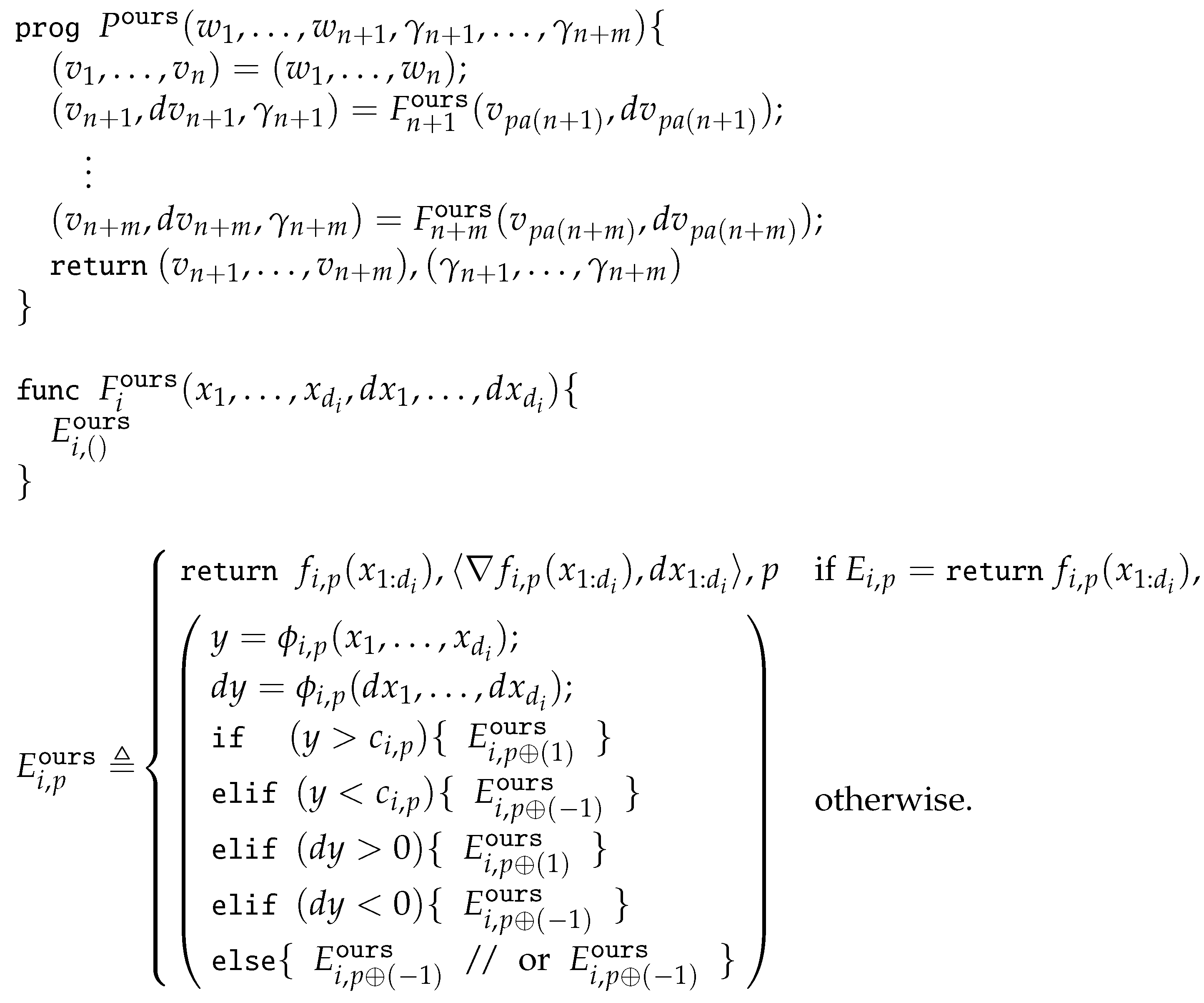
Algorithm 3 Forward pass of our algorithm

1: Input:  P, $(w_1,\cdots ,w_n)$ 2: Initialize:  Sample ${\delta }_i\sim \mathrm{Normal}(0,1)$, and set $(v_i,{dv}_i)=(w_i,{\delta }_i)$ for all $i\in \left[n\right]$ 3: for  $i=n+1,\dots ,n+m$  do 4:    Let $p=\left(\right)$ 5:     while  $p\notin {\mathsf{\Gamma }}_i$  do 6:       if  $({\varphi }_{i,p}\left(v_{pa\left(i\right)}\right)>c_{i,p})\vee ({\varphi }_{i,p}\left(v_{pa\left(i\right)}\right)=c_{i,p}\wedge {\varphi }_{i,p}\left(d{v}_{pa\left(i\right)}\right)>0)$  then 7:         $p=p\oplus \left(1\right)$ 8:      else if $({\varphi }_{i,p}\left(v_{pa\left(i\right)}\right)<c_{i,p})\vee ({\varphi }_{i,p}\left(v_{pa\left(i\right)}\right)=c_{i,p}\wedge {\varphi }_{i,p}\left(d{v}_{pa\left(i\right)}\right)<0)$  then 9:         $p=p\oplus (-1)$ 10:      else if ${\varphi }_{i,p}\left(v_{pa\left(i\right)}\right)=c_{i,p}\wedge {\varphi }_{i,p}\left(d{v}_{pa\left(i\right)}\right)=0$  then 11:         $p=p\oplus \left(s\right)$ for any $s\in \{-1,1\}$ 12:       end  if 13:     end  while 14:    Set ${\gamma }_i=p$, $v_i=f_{i,p}\left(v_{pa\left(i\right)}\right)$, and $d{v}_i=⟨\nabla f_{i,p}\left(v_{pa\left(i\right)}\right),d{v}_{pa\left(i\right)}⟩$ 15: end  for 16: return  $(v_1,\dots ,v_{n+m})$, $({\gamma }_{n+1},\dots ,{\gamma }_{n+m})$

We now illustrate the main idea behind our forward pass, which enables the backward pass to compute ${Dv}_{n+m,{\gamma }^{*}}\left(w\right)$ in Equation (2). As an example, consider a program with the following primitive functions: $F_{n+1},\cdots ,F_{n+m-1}$ are all analytic, and $F_{n+m}$ branches only once with ${\varphi }_{n+m,\left(\right)}(·)=\varphi (·)$ and $c_{n+m,\left(\right)}=0$. For notational simplicity, we use $u\left(w\right)=v_{pa(n+m)}\left(w\right)$.

If $\varphi \left(u\right(w\left)\right)>0$, then it is easy to observe that ${\gamma }_{n+m}^{*}=1$ from the continuity of $\varphi$ and u. Likewise, if $\varphi \left(u\right(w\left)\right)<0$, then ${\gamma }_{n+m}^{*}=-1$. In the case that $\varphi \left(u\right(w\left)\right)=0$, we use the following directional derivatives to determine ${\gamma }_{n+m}^{*}$:

$$\begin{array}{c}\hfill d{v}_i(w;\delta )\triangleq \underset{t\downarrow 0}{lim}\frac{v_i(w+t·\delta )-v_i\left(w\right)}{t}\end{array}$$

(3)

for $i\in [n+m-1]$, which can be easily computed using the chain rule. From the definition of $d{v}_i$, the linearity of $\varphi$, and the chain rule, it holds that

$$\begin{array}{c}\hfill \underset{t\downarrow 0}{lim}\frac{\varphi \left(u\right(w+t·\delta \left)\right)-\varphi \left(u\right(w\left)\right)}{t}=\sum _{j\in pa(n+m)}\frac{\partial \varphi \left(u\right(w\left)\right)}{\partial v_j\left(w\right)}·d{v}_j(w;\delta )=\varphi \left(du(w;\delta )\right),\end{array}$$

where $du(w;\delta )$ denotes the vector of all $d{v}_j(w;\delta )$ with $j\in pa(n+m)$. Then, by Taylor’s theorem, $\varphi \left(du\right(w;\delta \left)\right)>0$ (or $\varphi \left(du\right(w;\delta \left)\right)<0$) implies ${\gamma }_{n+m}^{*}=1$ (or ${\gamma }_{n+m}^{*}=-1$). In summary, if $\varphi \left(u\right(w\left)\right)\ne 0$ or $\varphi \left(du\right(w;\delta \left)\right)\ne 0$, then the exact ${\gamma }_{n+m}^{*}$ can be found, and hence, the backward pass (Algorithm 2) can correctly compute ${Dv}_{n+m,{\gamma }^{*}}\left(w\right)$ using ${\gamma }^{*}=(\left(\right),\dots ,\left(\right),{\gamma }_{n+m}^{*})$.

Now, we considered the only remaining case: $\varphi \left(u\right(w\left)\right)=0$ and $\varphi \left(du\right(w;\delta \left)\right)=0$. Unlike the previous cases, it is non-trivial here to find the correct ${\gamma }_{n+m}^{*}$ because the first-order Taylor series approximation does not provide any information about whether a small perturbation of w toward $\delta$ increases $\varphi \left(u\right(w\left)\right)$ or not. An important point, however, is that we do not need the exact ${\gamma }_{n+m}^{*}$ to compute an element of the Clarke subdifferential; instead, it suffices to compute ${Dv}_{n+m,{\gamma }^{*}}\left(w\right)$. Surprisingly, this can be performed by choosing an arbitrary piece of $F_{n+m}$, as shown below.

For simplicity, suppose that $\varphi \left(x\right)=x_1$, i.e., $\varphi \left(u\left(w\right)\right)=v_{i^{*}}\left(w\right)$ for some $i^{*}\in pa(n+m)$; the below argument can be easily extended to an arbitrary linear $\varphi$. Let ${\gamma }^{\alpha }=(\left(\right),\cdots ,\left(\right),\alpha )$ for $\alpha \in \left\{\right(-1),(1\left)\right\}$, i.e., ${\gamma }_{n+m}^{\alpha }=\alpha$. Then, for any $\alpha \in \left\{\right(-1),(1\left)\right\}$, we have

$$\begin{array}{c}\hfill {Dv}_{n+m,{\gamma }^{\alpha }}\left(w\right)=\sum _{j\in pa(n+m)\setminus \left\{i^{*}\right\}}\frac{\partial f_{n+m,\alpha }\left(u\left(w\right)\right)}{\partial v_j\left(w\right)}·{Dv}_j\left(w\right)\end{array}$$

(4)

almost surely, by the chain rule and the following result: $d{v}_{i^{*}}(w;\delta )=\varphi \left(du(w;\delta )\right)=0$ implies ${Dv}_{i^{*}}\left(w\right)=0$ almost surely (Lemma 5 in Section 4). Here, from the continuity and the definition of $F_{n+m}$, we must have $f_{n+m,\left(1\right)}=f_{n+m,(-1)}$ on the hyperplane $\{x\in {\mathbb{R}}^{d_{n+m}}:x_1=0\}$, and thus, $\partial f_{n+m,\left(1\right)}\left(x\right)/\partial x_j=\partial f_{n+m,(-1)}\left(x\right)/\partial x_j$ for any $x\in \{x\in {\mathbb{R}}^{d_{n+m}}:x_1=0\}$ and $j\in \left[d_{n+m}\right]\setminus \left\{1\right\}$. From this and $v_{i^{*}}\left(w\right)=\varphi \left(u\left(w\right)\right)=0$, we then obtain

$$\begin{array}{c}\hfill \frac{\partial f_{n+m,\left(1\right)}\left(u\left(w\right)\right)}{\partial v_j\left(w\right)}=\frac{\partial f_{n+m,(-1)}\left(u\left(w\right)\right)}{\partial v_j\left(w\right)}\end{array}$$

(5)

for all $j\in pa(n+m)\setminus \left\{i^{*}\right\}$. By combining Equations (4) and (5), we can finally conclude that

$$\begin{array}{c}\hfill {Dv}_{n+m,{\gamma }^{\left(1\right)}}\left(w\right)={Dv}_{n+m,{\gamma }^{(-1)}}\left(w\right)={Dv}_{n+m,{\gamma }^{*}}\left(w\right)\end{array}$$

almost surely, where the last equality is from the fact that ${\gamma }_{n+m}^{*}$ is either $\left(1\right)$ or $(-1)$. To summarize, if $\varphi \left(u\right(w\left)\right)=0$ and $\varphi \left(du\right(w;\delta \left)\right)=0$, we can compute the target element of the Clarke subdifferential (i.e., ${Dv}_{n+m,{\gamma }^{*}}\left(w\right)$) by choosing an arbitrary piece of $F_{n+m}$.

3.3. Forward Pass for Efficient Automatic Subdifferentiation

Our algorithm for computing an element of the Clarke subdifferential is based on the observation made in the previous section: it runs one forward pass (Algorithm 3) for computing $v_{n+1}\left(w\right),\cdots ,v_{n+m}\left(w\right)$ and some $\gamma \in \mathsf{\Gamma }$ such that ${Dv}_{n+m,\gamma }\left(w\right)={Dv}_{n+m,{\gamma }^{*}}\left(w\right)$ and one backward pass of AD (Algorithm 2) for computing ${Dv}_{n+m,\gamma }\left(w\right)$.

We now describe our forward pass procedure (Algorithm 3). First, it randomly samples a vector $\delta \in {\mathbb{R}}^n$ from a Gaussian distribution and initializes $d{v}_i={\delta }_i$ for all $i\in \left[n\right]$ (line 2). Then, it iterates for $i=n+1,\cdots ,n+m$ as follows. Given $v_1\left(w\right),\cdots ,v_{i-1}\left(w\right)$ and their directional derivatives $d{v}_1(w;\delta ),\cdots ,d{v}_{i-1}(w;\delta )$ with respect to $\delta$, lines 5–13 in Algorithm 3 find a proper piece ${\gamma }_i\in {\mathsf{\Gamma }}_i$ of $F_i$ by exploring its branches. If the condition in line 6 is satisfied, then it moves to the branch corresponding to ${\varphi }_{i,p}\left(v_{\left(i\right)}\left(w\right)\right)>c_{i,p}$ (line 7). It moves in a similar way if the condition in line 8 is satisfied. As in our example in Section 3.2, if ${\varphi }_{i,p}\left(v_{pa\left(i\right)}\left(w\right)\right)=c_{i,p}$ and ${\varphi }_{i,p}\left(d{v}_{pa\left(i\right)}(w;\delta )\right)=0$ (line 10), then our algorithm moves to an arbitrary branch (line 11). Once Algorithm 3 finds a proper piece ${\gamma }_i$ of $F_i$, it updates $v_i\left(w\right)$ and $d{v}_i(w;\delta )$ via the chain rule (line 14). Here, $v_i\left(w\right)$ can be correctly computed due to the continuity of $F_i$, while $d{v}_i(w;\delta )$ can also be correctly computed almost surely; see Lemma 8 in Section 4 for details. We remark that our algorithm is a generalization of the algorithm in [14]. The difference occurs in lines 10–11, where the existing algorithm deterministically chooses s based on some qualification condition [14].

As illustrated in Section 3.2, the piece $\gamma \in \mathsf{\Gamma }$ computed by our forward pass satisfies ${Dv}_{n+m,\gamma }\left(w\right)={Dv}_{n+m,{\gamma }^{*}}\left(w\right)$ almost surely, and hence, the backward pass using this $\gamma$ correctly computes ${Dv}_{n+m,{\gamma }^{*}}\left(w\right)$ almost surely, which is an element of the Clarke subdifferential. We formally state the correctness of our algorithm in the following theorem; its proof is given in Section 4.

Theorem 1. 

Suppose that Assumption 1 holds. Then, for any $w\in {\mathbb{R}}^n$, running Algorithm 3 and then Algorithm 2 returns an element of ${\partial }^c{v}_{n+m}\left(w\right)$ almost surely.

3.4. Computational Cost

In this section, we analyze the computational cost of our algorithm (both forward and backward passes) on a program P, compared to the cost of running P. Here, we only counted the cost of arithmetic operations and function evaluations and ignore the cost of memory read and write. We assumed that elementary operations ($+,\times ,\wedge ,\vee$), the comparison between two scalar values ($>,<,=$), and sampling a value from the standard normal distribution have a unit cost (e.g., cost$(+)=1$), while the cost for evaluating an analytic function f is represented by cost$\left(f\right)$. To denote the cost of evaluating a program P with an input w, we use cost$\left(P\right(w\left)\right)$. Likewise, for the cost of running our algorithm (i.e., Algorithms 2 and 3) on P and w, we use cost$\left(\mathrm{ours}\right(P,w\left)\right)$. We also assumed that memory read/write costs are included in our cost function. Under this setup, we bound the computational cost of our algorithm in Theorem 2.

Theorem 2. 

Suppose that $\mathrm{cost}\left(P\right(w\left)\right)\ge n$ for all $w\in {\mathbb{R}}^n$. Then, for any program P and its input $w\in {\mathbb{R}}^n$, $\mathrm{cost}\left(\mathrm{ours}\right(P,w\left)\right)\le \kappa ·\mathrm{cost}\left(P\right(w\left)\right)$ where

$$\begin{array}{cc}\hfill \kappa \triangleq & 1+\underset{i\in [n+m]\setminus \left[n\right]}{max}{\kappa }_i,\hfill \\ \hfill {\kappa }_i\triangleq & \frac{{max}_{p\in {\mathsf{\Gamma }}_i}2\mathrm{cost}(\nabla f_{i,p})+\mathrm{cost}\left(f_{i,p}\right)+4d_i+4\mathrm{len}\left(p\right)+2{\sum }_{j=1}^{\mathrm{len}\left(p\right)}\mathrm{cost}\left({\varphi }_{i,p_{:j}}\right)}{{min}_{q\in {\mathsf{\Gamma }}_i}\mathrm{cost}\left(f_{i,q}\right)+\mathrm{len}\left(q\right)+{\sum }_{j=1}^{\mathrm{len}\left(q\right)}\mathrm{cost}\left({\varphi }_{i,q_{:j}}\right)}.\hfill \end{array}$$

(6)

The assumption in Theorem 2 is mild since it is satisfied if at least one distinct operation is applied to each input for evaluating P. The proof of Theorem 2 is presented in Section 5, where we use program representations of Algorithms 2 and 3 (see Figure 4 and Figure 5 in Section 3.4 for the details).

Figure 4. A program $P^{\mathtt{ADB}}$ implementing the backward pass of AD (Algorithm 2).

Figure 5. A program $P^{\mathtt{ours}}$ implementing Algorithm 3. Here, $x_{1:d_i}=(x_1,\cdots ,x_{d_i})$.

Suppose that, for each $i\in [n+m]\setminus \left[n\right]$, $d_i$ and ${max}_{p\in {\mathsf{\Gamma }}_i}\mathrm{len}\left(p\right)$ (i.e., the arity and the maximum branch depth of $f_i$) are independent of n. This condition holds in many practical cases: e.g., the absolute value function has $d_i=1$ and ${max}_{p\in {\mathsf{\Gamma }}_i}\mathrm{len}\left(p\right)=1$; $max\{·,·\}$ has $d_i=2$ and ${max}_{p\in {\mathsf{\Gamma }}_i}\mathrm{len}\left(p\right)=1$. Under this mild condition, $\mathrm{cost}\left(f_{i,p}\right)$, $\mathrm{cost}(\nabla f_{i,p})$, and $\mathrm{cost}\left({\varphi }_{i,p_{:j}}\right)$ are independent of n, and thus, ${\kappa }_i$ does so because the numerator in the definition of ${\kappa }_i$ is independent of n and the denominator is at least one (as $\mathrm{cost}\left(f_{i,q}\right)\ge 1$). This implies that $\kappa$ is independent of the input dimension n under the above condition.

In practical setups with large n, the computational cost of our algorithm can be much smaller than that of existing algorithms based on the lexicographic subdifferential [17,18,19,20]. For example, modern neural networks have more than a million parameters (i.e., n), where the cost for computing the gradient of each piece in the activation functions (i.e., $\mathrm{cost}(\nabla f_{i,p})$) is typically bounded by $O\left(\mathrm{cost}\left(f_{i,p}\right)\right)$. Further, the depth of branches in these activation functions is often bounded by a constant (e.g., the depth is one for ReLU). Hence, for those networks, $\kappa =O\left(1\right)$, and our algorithm does not incur much computational overhead. On the other hand, lexicographic-subdifferential-based approaches require at least n computations of $P\left(w\right)$ [17,18,19,20], which may not be practical when n is large.

4. Proof of Theorem 1

In this section, we prove Theorem 3 under the setup that $\delta$ in Algorithm 3 is given instead of randomly sampled. This theorem directly implies Theorem 1 since the statement of Theorem 3 holds for almost every $\delta$ and the proof of Theorem 1 requires showing the same statement almost surely, where the randomness comes from $\delta$ following an Isotropic Gaussian distribution. Namely, proving Theorem 3 suffices for proving Theorem 1. We note that all results in this section are under Assumption 1.

Theorem 3. 

Given $w\in {\mathbb{R}}^n$, Algorithms 3 and 2 compute an element of ${\partial }^c{v}_{n+m}\left(w\right)$ for almost every $\delta \in {\mathbb{R}}^n$.

4.1. Additional Notations

We frequently use the following shorthand notations: the set of indices of branches:

$${\mathcal{I}}_{br}\triangleq \{i\in [n+m]:|{\mathsf{\Gamma }}_i|>1\}$$

and an auxiliary index set:

$${\mathrm{Idx}}_i\triangleq \{(j,p):p\in {\mathsf{\Gamma }}_i,j\in \left[\mathrm{len}\left(p\right)\right]\}.$$

For $\gamma \in \mathsf{\Gamma }$, $i\in [n+m]\setminus \left[n\right]$, and $(j,p)\in {\mathrm{Idx}}_i$, we use

$$\begin{array}{cc}\hfill {\varphi }_{i,p_{:j}}^{\gamma }\left(w\right)\triangleq & {\varphi }_{i,p_{:j}}\left(v_{pa\left(i\right),\gamma }\left(w\right)\right).\hfill \end{array}$$

Note that $v_{i,\gamma }$ and ${\varphi }_{i,p_{:j}}^{\gamma }$ are analytic (and, therefore, differentiable) for all $\gamma \in \mathsf{\Gamma }$, $i\in [n+m]\setminus \left[n\right]$, and $(j,p)\in {\mathrm{Idx}}_i$. We next define the set of pieces reachable by our algorithm (Algorithm 3) with inputs $w=(w_1,\cdots ,w_n),\delta =({\delta }_1,\cdots ,{\delta }_n)\in {\mathbb{R}}^n$ as $\mathsf{\Gamma }(w,\delta )$:

$$\begin{array}{cc}\hfill & \mathsf{\Gamma }(w,\delta )\triangleq \{\gamma \in \mathsf{\Gamma }:{\gamma }_{i,j}\in {\mathcal{C}}_{i,j}^{\gamma }(w;\delta )\forall i\in {\mathcal{I}}_{br},\forall j\in \left[\mathrm{len}\left({\gamma }_i\right)\right]\},\mathrm{where}\hfill \\ \hfill & {\mathcal{C}}_{i,j}^{\gamma }(w;\delta )\triangleq \left\{\begin{array}{cc}\left\{1\right\}\hfill & \mathrm{if}\left({\varphi }_{i,{\gamma }_{i,:j}}\left(v_{pa\left(i\right),\gamma }\left(w\right)\right)=c_{i,{\gamma }_{i,:j}}\wedge {\varphi }_{i,{\gamma }_{i,:j}}\left(d{v}_{pa\left(i\right),\gamma }(w;\delta )\right)>0\right)\hfill \\ \hfill & \vee \left({\varphi }_{i,{\gamma }_{i,:j}}\left(v_{pa\left(i\right)}^{\gamma }\right)>c_{i,{\gamma }_{i,:j}}\right)\hfill \\ \{-1\}\hfill & \mathrm{if}\left({\varphi }_{i,{\gamma }_{i,:j}}\left(v_{pa\left(i\right),\gamma }\left(w\right)\right)=c_{i,{\gamma }_{i,:j}}\wedge {\varphi }_{i,{\gamma }_{i,:j}}\left(d{v}_{pa\left(i\right),\gamma }(w;\delta )\right)<0\right)\hfill \\ \hfill & \vee \left({\varphi }_{i,{\gamma }_{i,:j}}\left(v_{pa\left(i\right)}^{\gamma }\right)<c_{i,{\gamma }_{i,:j}}\right)\hfill \\ \{-1,1\}\hfill & \mathrm{if}\left({\varphi }_{i,{\gamma }_{i,:j}}\left(v_{pa\left(i\right),\gamma }\left(w\right)\right)=c_{i,{\gamma }_{i,:j}}\wedge {\varphi }_{i,{\gamma }_{i,:j}}\left(d{v}_{pa\left(i\right),\gamma }(w;\delta )\right)=0\right)\hfill \end{array}\right..\hfill \end{array}$$

4.2. Technical Claims

Lemma 1. 

For any open $\mathcal{O}\subset \mathbb{R}$, for any analytic, but non-constant $f:\mathcal{O}\to \mathbb{R}$, and for any $x\in \mathcal{O}$, there exists $\epsilon >0$ such that

$$\begin{array}{c}\hfill f\left(x\right)\notin f\left(\right[x-\epsilon ,x+\epsilon ]\setminus \{x\left\}\right).\end{array}$$

Furthermore, f is strictly monotone on $[x,x+\epsilon ]$ and strictly monotone on $[x-\epsilon ,x]$.

Proof Lemma 1. 

Without loss of generality, suppose that $f\left(x\right)=0$. Since f is analytic, f is infinitely differentiable and can be represented by the Taylor series on $(x-\delta ,x+\delta )$ for some $\delta >0$:

$$\begin{array}{c}\hfill f\left(z\right)=\sum _{i=0}^{\infty }\frac{f^{\left(i\right)}\left(x\right)}{i!}{(z-x)}^i\end{array}$$

where $f^{\left(i\right)}$ denotes the i-th derivative of f. Since f is non-constant, there exists $i\in \mathbb{N}$ such that $f^{\left(i\right)}\left(x\right)\ne 0$. Let $i^{*}$ be the minimum such i. Then, by Taylor’s theorem, $f\left(z\right)=\frac{f^{\left(i^{*}\right)}\left(x\right)}{i^{*}!}{(z-x)}^{i^{*}}{+o\left(\right|z-x|}^{i^{*}})$.

Consider the case that $f^{\left(i\right)}\left(x\right)>0$ and $i^{*}$ is odd. Then, we can choose $\epsilon \in (0,\delta )$ so that

$$\begin{array}{cc}\hfill & f^{\left(1\right)}\left(z\right)<0\mathrm{on}[x-\epsilon ,x)\mathrm{and}{f}^{\left(1\right)}\left(z\right)>0\mathrm{on}(x,x+\epsilon ]\hfill \end{array}$$

i.e., f is strictly increasing on $[x-\epsilon ,x+\epsilon ]$ (e.g., by the mean value theorem), and hence, $f\left(x\right)\notin f\left(\right[x-\epsilon ,x+\epsilon ]\setminus \{x\left\}\right)$. One can apply a similar argument to the cases that $f^{\left(i\right)}\left(x\right)<0$ and $i^{*}$ is odd, $f^{\left(i\right)}\left(x\right)>0$ and $i^{*}$ is even, and $f^{\left(i\right)}\left(x\right)<0$ and $i^{*}$ is even. This completes the proof of Lemma 1.    □

Lemma 2 

(Proposition 0 in [35]). For any $n\in \mathbb{N}$, for any open connected $\mathcal{O}\subset {\mathbb{R}}^n$, and for any real analytic $f:\mathcal{O}\to \mathbb{R}$, if ${\mu }_n\left(\mathit{zero}\left(f\right)\right)>0$, then $f\left(x\right)=0$ for all $x\in \mathcal{O}$.

Lemma 3. 

For any $n\in \mathbb{N}$, for any open connected $\mathcal{O}\subset {\mathbb{R}}^n$, and for any real analytic $f,g:\mathcal{O}\to \mathbb{R}$, if ${\mu }_n\left(\mathit{zero}(f-g)\right)>0$, then $f\left(x\right)=g\left(x\right)$ for all $x\in \mathcal{O}$.

Proof Lemma 3. 

The proof directly follows from Lemma 2.    □

4.3. Technical Assumptions

Assumption 2. 

Given $w\in {\mathbb{R}}^n$, $\delta \in {\mathbb{R}}^n$ satisfies the following: for any $\gamma \in \mathsf{\Gamma }$, $i\in {\mathcal{I}}_{br}$, and $(j,p)\in {\mathrm{Idx}}_i$, if ${\varphi }_{i,p_{:j}}^{\gamma }$ is not a constant function, then

$$\begin{array}{c}\hfill {\varphi }_{i,p_{:j}}^{\gamma }(w+t·\delta )\mathit{is}\mathit{not}a\mathit{constant}\mathit{function}\mathit{in}t\in \mathbb{R}.\end{array}$$

Assumption 3. 

Given $w\in {\mathbb{R}}^n$, $\delta \in {\mathbb{R}}^n$ satisfies the following: for any $\gamma \in \mathsf{\Gamma }$, $i\in {\mathcal{I}}_{br}$, and $(j,p)={\mathrm{Idx}}_i$,

$$\begin{array}{c}\hfill ⟨\delta ,{D\varphi }_{i,p_{:j}}^{\gamma }\left(w\right)⟩=0\mathit{if}\mathit{and}\mathit{only}\mathit{if}{D\varphi }_{i,p_{:j}}^{\gamma }\left(w\right)=\overrightarrow{0}.\end{array}$$

4.4. Technical Lemmas

Lemma 4. 

Given $w\in {\mathbb{R}}^n$, almost every $\delta \in {\mathbb{R}}^n$ satisfies Assumption 2.

Proof of Lemma 4. 

Since $\left|\mathsf{\Gamma }\right|<\infty$, if the set of $\delta$ that does not satisfy Assumption 2 has a non-zero measure, then there exist $\gamma \in \mathsf{\Gamma }$, $i\in {\mathcal{I}}_{br}$, and $(j,p)\in {\mathsf{Idx}}_i$ such that ${\varphi }_{i,p_{:j}}^{\gamma }$ is not a constant function and

$$\begin{array}{c}\hfill {\mu }_n\left(\mathcal{S}\triangleq \{\delta \in {\mathbb{R}}^n:{\varphi }_{i,p_{:j}}^{\gamma }(w+t·\delta )\mathrm{is}\mathrm{a}\mathrm{constant}\mathrm{function}\mathrm{in}t\in \mathbb{R}\}\right)>0.\end{array}$$

Without loss of generality, suppose that ${\varphi }_{i,p_{:j}}^{\gamma }\left(w\right)=0$. Then, from the definition of $\mathcal{S}$, $\mathcal{S}$ is contained in the zero set:

$$\begin{array}{c}\hfill \mathit{zero}\left(\tilde{\varphi }\right)\triangleq \{u\in \mathbb{R}:\tilde{\varphi }\left(u\right)=0\}\end{array}$$

of an analytic function $\tilde{\varphi }:{\mathbb{R}}^W\to \mathbb{R}$ defined as

$$\begin{array}{c}\hfill \tilde{\varphi }\left(u\right)\triangleq {\varphi }_{i,p_{:j}}^{\gamma }(w+u).\end{array}$$

Namely, ${\mu }_n\left(\mathit{zero}\left(\tilde{\varphi }\right)\right)\ge {\mu }_n\left(\mathcal{S}\right)>0$. However, from Lemma 2, $\tilde{\varphi }$ must be a constant function, which contradicts our assumption that ${\varphi }_{i,p_{:j}}^{\gamma }$ is not a constant function. This completes the proof of Lemma 4.    □

Lemma 5. 

Given $w\in {\mathbb{R}}^n$, almost every $\delta \in {\mathbb{R}}^n$ satisfies Assumption 3.

Proof of Lemma 5. 

Since ${D\varphi }_{i,p_{:j}}^{\gamma }\left(w\right)=\overrightarrow{0}$ implies $⟨\delta ,{\varphi }_{i,p_{:j}}^{\gamma }\left(w\right)⟩=0$ for all $\delta \in {\mathbb{R}}^n$, we prove the converse. Suppose that ${D\varphi }_{i,p_{:j}}^{\gamma }\left(w\right)\ne \overrightarrow{0}$. Since the set $\{\delta \in {\mathbb{R}}^n:⟨\delta ,{D\varphi }_{i,p_{:j}}^{\gamma }\left(w\right)⟩=0\}$ has zero measure under ${D\varphi }_{i,p_{:j}}^{\gamma }\left(w\right)\ne \overrightarrow{0}$,

$$\begin{array}{c}\hfill \bigcup _{\gamma \in \mathsf{\Gamma },i\in {\mathcal{I}}_{br},(j,p)\in {\mathrm{Idx}}_i:{D\varphi }_{i,p_{:j}}^{\gamma }\left(w\right)\ne \overrightarrow{0}}\{\delta \in {\mathbb{R}}^n:⟨\delta ,{D\varphi }_{i,p_{:j}}^{\gamma }\left(w\right)⟩=0\}\end{array}$$

also has zero measure. This completes the proof of Lemma 5.    □

Lemma 6. 

For $i\in {\mathcal{I}}_{br}$ and $p\in {\mathsf{\Gamma }}_i$, suppose that $x\in {\mathbb{R}}^{d_i}$ satisfies one of the following for all $j\in \left[\mathrm{len}\right(p\left)\right]$:

• $\mathrm{sign}({\varphi }_{i,p_{:j}}\left(x\right)-c_{i,p_{:j}})=p_j$;
• ${\varphi }_{i,p_{:j}}\left(x\right)=c_{i,p_{:j}}$.

Then,$x\in \mathrm{cl}\left({\mathcal{X}}_{i,p}\right)$.

Proof of Lemma 6. 

Without loss of generality, assume that $x\notin {\mathcal{X}}_{i,p}$. Since we assumed ${\mathcal{X}}_{i,p}\ne \varnothing$ by Assumption 1, there exists $y\in {\mathcal{X}}_{i,p}$, i.e., $\mathrm{sign}({\varphi }_{i,p_{:j}}\left(y\right)-c_{i,p_{:j}})=p_j$ for all $j\in \left[\mathrm{len}\right(p\left)\right]$. Define

$$\begin{array}{c}\hfill \mathcal{I}\triangleq \{j\in \left[\mathrm{len}\left(p\right)\right]:{\varphi }_{i,p_{:j}}\left(x\right)=c_{i,p_{:j}}\}.\end{array}$$

Since ${\varphi }_{i,p_{:j}}$ is linear, for $z=y-x$ and for any $j\in \mathcal{I}$, we have

$$\begin{array}{c}\hfill \mathrm{sign}\left({\varphi }_{i,p_{:j}}\left(z\right)\right)=p_j.\end{array}$$

This implies that, for any $t>0$ and $j\in \mathcal{I}$, it holds that

$$\begin{array}{c}\hfill \mathrm{sign}\left({\varphi }_{i,p_{:j}}(x+t·z)\right)=p_j.\end{array}$$

(7)

Since $|{\varphi }_{i,p_{:j}}\left(x\right)-c_{i,p_{:j}}|>0$ and $\mathrm{sign}\left({\varphi }_{i,p_{:j}}\left(x\right)\right)=p_j$ for all $j\in \left[\mathrm{len}\right(p\left)\right]\setminus \mathcal{I}$ by the definition of $\mathcal{I}$, there exists $s>0$ such that

$$\begin{array}{c}\hfill |{\varphi }_{i,p_{:j}}(x+t·z)-c_{i,p_{:j}}|>0\mathrm{and}\mathrm{sign}\left({\varphi }_{i,p_{:j}}(x+t·z)\right)=p_j\end{array}$$

(8)

for all $t\in [0,s]$ and $j\in \left[\mathrm{len}\right(p\left)\right]\setminus \mathcal{I}$. Combining Equations (7) and (8) implies that $x+t·z\in {\mathcal{X}}_{i,p}$ for all $t\in (0,s]$, i.e., x is a limit point of ${\mathcal{X}}_{i,p}$. This completes the proof of lem:closure    □

4.5. Key Lemmas

Lemma 7. 

For any $w\in {\mathbb{R}}^n$ and for any $\delta \in {\mathbb{R}}^n$ satisfying Assumption 2, there exist $s^{*}>0$ and ${\gamma }^{*}\in \mathsf{\Gamma }(w,\delta )$ such that

$$\begin{array}{c}\hfill w+t·\delta \in \mathrm{int}\left({\mathcal{W}}_{{\gamma }^{*}}\right)\mathit{for}\mathit{all}t\in (0,s^{*}).\end{array}$$

Proof of Lemma 7. 

We first define some notations: for an analytic function $f:\mathbb{R}\to \mathbb{R}$ and $t\in \mathbb{R}$,

$$\begin{array}{cc}\hfill {\varphi }_{i,p_{:j}}^{\gamma ,w,\delta }\left(t\right)\triangleq & {\varphi }_{i,p_{:j}}^{\gamma }(w+t·\delta ),\hfill \\ \hfill \mathrm{dir}\left(f\right)\triangleq & \left\{\begin{array}{cc}{s}^{\prime }\hfill & \mathrm{if}{s}^{\prime }={sup}_{s\ge 0}\left\{f\right(0)\mathrm{is}\mathrm{strictly}\mathrm{increasing}\mathrm{on}[0,s]\}>0\hfill \\ s^{″}\hfill & \mathrm{if}{s}^{″}={sup}_{s\ge 0}\left\{f\right(0)\mathrm{is}\mathrm{strictly}\mathrm{decreasing}\mathrm{on}[0,s]\}>0\hfill \\ \perp \hfill & \mathrm{otherwise}\hfill \end{array}\right..\hfill \end{array}$$

Under Assumption 2 and by Lemma 1, one can observe that, for any $i\in {\mathcal{I}}_{br}$, $p={\gamma }_i$, and $j\in \left[\mathrm{len}\right(p\left)\right]$, $\mathrm{dir}\left({\varphi }_{i,p_{:j}}^{\gamma ,w,\delta }\right)=\perp$ if and only if ${\varphi }_{i,p_{:j}}^{\gamma }$ is a constant function. In addition, from Lemma 1, if ${\varphi }_{i,p_{:j}}^{\gamma }$ is not a constant function, then $\mathrm{dir}\left({\varphi }_{i,p_{:j}}^{\gamma ,w,\delta }\right)>0$. Using Algorithm 4, we iteratively construct ${\gamma }^{*}\in \mathsf{\Gamma }(w,\delta )$ and update $s^{*}>0$ for each $i\in {\mathcal{I}}_{br}$ so that

$$\begin{array}{c}\hfill w+t·\delta \in \mathrm{int}\left({\mathcal{W}}_{{\gamma }^{*}}\right)\mathrm{for}\mathrm{all}t\in (0,s^{*}).\end{array}$$

Under our construction of ${\gamma }^{*}$, one can observe that ${\gamma }^{*}\in \mathsf{\Gamma }(w,\delta )$. From our choice of $s^{*}$, for any $i\in {\mathcal{I}}_{br}$, $j\in \left[\mathrm{len}\right(p\left)\right]$, and for $s_{i,j}=\mathrm{dir}\left({\varphi }_{i,{\gamma }_{i,:j}^{*}}^{{\gamma }^{*},w,\delta }\right)$, the following statements hold:

• If $s_{i,j}\ne \perp$, then ${\varphi }_{i,{\gamma }_{i,:j}^{*}}^{{\gamma }^{*},w,\delta }\left((0,s^{*})\right)$ is open since ${\varphi }_{i,{\gamma }_{i,:j}^{*}}^{{\gamma }^{*},w,\delta }$ is strictly monotone on $(0,s^{*})$;
• If $s_{i,j}=\perp$, then ${\varphi }_{i,{\gamma }_{i,:j}^{*}}^{{\gamma }^{*},w,\delta },{\varphi }_{i,{\gamma }_{i,:j}^{*}}^{{\gamma }^{*}}$ are constant functions (i.e., ${\varphi }_{i,{\gamma }_{i,:j}^{*}}^{{\gamma }^{*},w,\delta }\left((0,s^{*})\right)$ is a constant) due to Assumption 2.

For any $t\in (0,s^{*})$, we have $w+t·\delta \in \mathcal{O}\subset {\mathcal{W}}_{{\gamma }^{*}}$, where

$$\begin{array}{cc}\hfill & \mathcal{O}\triangleq \left(\bigcap _{i,j:z_{i,j}=\perp }{\left({\varphi }_{i,{\gamma }_{i,:j}^{*}}^{{\gamma }^{*}}\right)}^{-1}\left({\varphi }_{i,{\gamma }_{i,:j}^{*}}^{{\gamma }^{*},w,\delta }\left((0,s^{*})\right)\right)\right)\cap \left(\bigcap _{i,j:z_{i,j}\ne \perp }{\left({\varphi }_{i,{\gamma }_{i,:j}^{*}}^{{\gamma }^{*}}\right)}^{-1}\left({\varphi }_{i,{\gamma }_{i,:j}^{*}}^{{\gamma }^{*},w,\delta }\left((0,s^{*})\right)\right)\right).\hfill \end{array}$$

Here, $\mathcal{O}$ is open since each term for the intersection in the above equation is open; it is ${\mathbb{R}}^n$ if $s_{i,j}=\perp$, and it is an inverse image of a continuous function of an open set otherwise. This completes the proof of Lemma 7.    □

Algorithm 4 Construction of ${\gamma }^{*}$ and $s^{*}$

Input: P, $(w_1,\cdots ,w_n)$, $({\delta }_1,\dots ,{\delta }_n)$ Initialize: $(v_1,\cdots ,v_n)=(w_1,\dots ,w_n)$, ${dv}_i={\delta }_i$ for all $i\in \left[n\right]$, $s^{*}=\infty$, ${\gamma }^{*}=\left(\left(\right),\cdots ,\left(\right)\right)$ for  $i=n+1,\dots ,n+m$  do    Let $x=v_{pa\left(i\right)}$, $dx=d{v}_{pa\left(i\right)}$, and $p=\left(\right)$     while  $p\notin {\mathsf{\Gamma }}_i$  do      Set $y={\varphi }_{i,p}\left(x\right)$ and $s=\mathrm{dir}\left({\varphi }_{i,p}^{{\gamma }^{*},w,\delta }\right)$       if  $s=\perp \wedge y>c_{i,p}$  then         $p=p\oplus 1$ else if $s=\perp \wedge y\le c_{i,p}$then         $p=p\oplus (-1)$ else if $s\ne \perp \wedge y>c_{i,p}$ then         $p=p\oplus 1$ and $\epsilon =min\{|{\varphi }_{i,p}^{{\gamma }^{*},w,\delta }\left(s\right)-y|,y-c_{i,p}\}$         $\left\{s^{\prime }\right\}={\left({\varphi }_{i,p}^{{\gamma }^{*},w,\delta }\right)}^{-1}(y+z·\epsilon )\cap [0,s]$ and $s^{*}=min\{s^{*},s^{\prime }\}$ else if $s\ne \perp \wedge y<c_{i,p}$ then         $p=p\oplus (-1)$ and $\epsilon =min\{|{\varphi }_{i,p}^{{\gamma }^{*},w,\delta }\left(s\right)-y|,c_{i,p}-y\}$         $\left\{s^{\prime }\right\}={\left({\varphi }_{i,p}^{{\gamma }^{*},w,\delta }\right)}^{-1}(y+z·\epsilon )\cap [0,s]$ and $s^{*}=min\{s^{*},s^{\prime }\}$ else if $s\ne \perp \wedge y=c_{i,p}$ then         $p=p\oplus \mathrm{sign}\left(z\right)$ and $s^{*}=min\{s^{*},s\}$       end  if      Set ${\gamma }_i^{*}=p$ and $v_i=f_{i,{\gamma }_i^{*}}\left(x\right)$     end  while end  for return  ${\gamma }^{*}$, $s^{*}$

Corollary 1. 

For any $w\in {\mathbb{R}}^n$ and for any $\delta \in {\mathbb{R}}^n$ satisfying Assumption 2, there exist $s^{*}>0$ and ${\gamma }^{*}\in \mathsf{\Gamma }(w,\delta )$ such that

$$\begin{array}{c}\hfill {Dv}_{n+m}(w+t·\delta )={Dv}_{n+m,{\gamma }^{*}}(w+t·\delta )\mathit{for}\mathit{all}t\in (0,s^{*}).\end{array}$$

Proof of Corollary 1. 

This corollary directly follows from Lemma 7.    □

Lemma 8. 

For any $w\in {\mathbb{R}}^n$ and for any $\delta$ satisfying Assumption 3, it holds that

$${Dv}_{n+m,{\gamma }^{\prime }}\left(w\right)={Dv}_{n+m,{\gamma }^{″}}\left(w\right)\mathit{for}\mathit{all}{\gamma }^{\prime },{\gamma }^{″}\in \mathsf{\Gamma }(w,\delta ).$$

Proof of Lemma 8. 

We use the mathematical induction on i to show that $v_{i,{\gamma }^{\prime }}\left(w\right)=v_{i,{\gamma }^{″}}\left(w\right)$ and ${Dv}_{i,{\gamma }^{\prime }}\left(w\right)={Dv}_{i,{\gamma }^{″}}\left(w\right)$ for all $i\in [n+m]$. The base case is trivial: $v_{i,{\gamma }^{\prime }}\left(w\right)=v_{i,{\gamma }^{″}}\left(w\right)$ and ${Dv}_{i,{\gamma }^{\prime }}\left(w\right)={Dv}_{i,{\gamma }^{″}}\left(w\right)$ for all $i\in \left[n\right]$. Hence, suppose that $i\in {\mathcal{I}}_{br}$ since the case that $i\in [n+m]\setminus (\left[n\right]\cup {\mathcal{I}}_{br})$ is also trivial. Then, by the induction hypothesis, we have $v_{j,{\gamma }^{\prime }}\left(w\right)=v_{j,{\gamma }^{″}}\left(w\right)$ and ${Dv}_{j,{\gamma }^{\prime }}\left(w\right)={Dv}_{j,{\gamma }^{″}}\left(w\right)$ for all $j\in [i-1]$. For notational simplicity, we denote $x_j\triangleq v_{j,{\gamma }^{\prime }}\left(w\right)=v_{j,{\gamma }^{″}}\left(w\right)$ and $d{x}_j\triangleq d{v}_{j,{\gamma }^{\prime }}(w;\delta )=d{v}_{j,{\gamma }^{″}}(w;\delta )$ for all $j\in [i-1]$.

Let $p^{\prime }={\gamma }_i^{\prime }$ and $p^{″}={\gamma }_i^{″}$. First, by Lemma 6, the definition of $\mathsf{\Gamma }(w,\delta )$, and the induction hypothesis, we have

$$\begin{array}{c}\hfill x_{pa\left(i\right)}\in \mathrm{cl}\left({\mathcal{X}}_{i,p^{\prime }}\right)\cap \mathrm{cl}\left({\mathcal{X}}_{i,p^{″}}\right).\end{array}$$

Due to the continuity of $F_i$, this implies that

$$\begin{array}{c}\hfill v_{i,{\gamma }^{\prime }}\left(w\right)=f_{i,p^{\prime }}\left(x_{pa\left(i\right)}\right)=f_{i,p^{″}}\left(x_{pa\left(i\right)}\right)=v_{i,{\gamma }^{″}}\left(w\right).\end{array}$$

Now, it remains to show ${Dv}_{i,{\gamma }^{\prime }}\left(w\right)={Dv}_{i,{\gamma }^{″}}\left(w\right)$. To this end, we define the following:

$$\begin{array}{cc}\hfill \mathcal{I}& \triangleq \left\{(j,p)\in {\mathrm{Idx}}_i:{\varphi }_{i,p_{:j}}\left(d{x}_{pa\left(i\right)}\right)=0\right\},\hfill \\ \hfill \mathcal{S}& \triangleq \left\{x\in {\mathbb{R}}^{d_i}:{\varphi }_{i,p_{:j}}\left(x\right)=0\mathrm{for}\mathrm{all}(j,p)\in \mathcal{I}\right\}.\hfill \end{array}$$

From the definition of $\mathcal{S}$ and $\mathcal{I}$, $d{x}_{pa\left(i\right)}\in \mathcal{S}$. Furthermore, by Assumption 3, for any $(j,p)\in {\mathrm{Idx}}_i$ and $\gamma \in \{{\gamma }^{\prime },{\gamma }^{″}\}$, we have ${\varphi }_{i,p_{:j}}\left(d{v}_{pa\left(i\right),\gamma }(w;\delta )\right)=0$ if and only if ${D\varphi }_{i,p_{:j}}\left(v_{pa\left(i\right),\gamma }\left(w\right)\right)=\overrightarrow{0}$, i.e., $\partial {\varphi }_{i,p_{:j}}\left(v_{pa\left(i\right),\gamma }\left(w\right)\right)/\partial w_{\ell }={\varphi }_{i,p_{:j}}(\partial v_{pa\left(i\right),\gamma }\left(w\right)/\partial w_{\ell })=0$ for all $\ell \in \left[n\right]$. Therefore, since $d{x}_{pa\left(i\right)}\in \mathcal{S}$, it holds that

$$\begin{array}{c}\hfill \frac{\partial v_{pa\left(i\right),{\gamma }^{\prime }}\left(w\right)}{\partial w_{\ell }},\frac{\partial v_{pa\left(i\right),{\gamma }^{″}}\left(w\right)}{\partial w_{\ell }}\in \mathcal{S}\mathrm{for}\mathrm{all}\ell \in \left[n\right].\end{array}$$

In addition, due to the identities

$$\begin{array}{cc}\hfill & {Dv}_{i,{\gamma }^{\prime }}\left(w\right)={Df}_{i,p^{\prime }}\left(v_{pa\left(i\right),{\gamma }^{\prime }}\left(w\right)\right),{Dv}_{i,{\gamma }^{″}}\left(w\right)={Df}_{i,p^{″}}\left(v_{pa\left(i\right),{\gamma }^{″}}\left(w\right)\right),\hfill \\ \hfill & \frac{\partial f_{i,p^{\prime }}\left(v_{pa\left(i\right),{\gamma }^{\prime }}\left(w\right)\right)}{\partial w_{\ell }}=⟨\nabla f_{i,p^{\prime }}\left(x_{pa\left(i\right)}\right),\frac{\partial v_{pa\left(i\right),{\gamma }^{\prime }}\left(w\right)}{\partial w_{\ell }}⟩,\hfill \\ \hfill & \frac{\partial f_{i,p^{″}}\left(v_{pa\left(i\right),{\gamma }^{″}}\left(w\right)\right)}{\partial w_{\ell }}=⟨\nabla f_{i,p^{″}}\left(x_{pa\left(i\right)}\right),\frac{\partial v_{pa\left(i\right),{\gamma }^{″}}}{\partial w_{\ell }}⟩,\hfill \end{array}$$

showing the following stronger statement suffices for proving Lemma 8:

$$\begin{array}{c}\hfill ⟨\nabla f_{i,p^{\prime }}\left(x_{pa\left(i\right)}\right),z⟩=⟨\nabla f_{i,p^{″}}\left(x_{pa\left(i\right)}\right),z⟩\mathrm{for}\mathrm{all}z\in \mathcal{S}.\end{array}$$

(9)

By Lemma 1 and the induction hypothesis ($d{v}_{pa\left(i\right),{\gamma }^{\prime }}=d{v}_{pa\left(i\right),{\gamma }^{″}}$), there exists $s>0$ such that, for any $t\in (0,s)$ and $(j,p)\in {\mathrm{Idx}}_i$ and for $z_t=x_{pa\left(i\right)}+t·d{x}_{pa\left(i\right)}$,

$$\begin{array}{cc}\hfill & {\varphi }_{i,p_{:j}}\left(z_t\right)>c_{i,p_{:j}}\mathrm{if}({\varphi }_{i,p_{:j}}\left(x_{pa\left(i\right)}\right)=c_{i,p_{:j}}\wedge {\varphi }_{i,p_{:j}}\left(d{x}_{pa\left(i\right)}\right)>0)\vee ({\varphi }_{i,p_{:j}}\left(x_{pa\left(i\right)}\right)>c_{i,p_{:j}}),\hfill \\ \hfill & {\varphi }_{i,p_{:j}}\left(z_t\right)<c_{i,p_{:j}}\mathrm{if}({\varphi }_{i,p_{:j}}\left(x_{pa\left(i\right)}\right)=c_{i,p_{:j}}\wedge {\varphi }_{i,p_{:j}}\left(d{x}_{pa\left(i\right)}\right)<0)\vee ({\varphi }_{i,p_{:j}}\left(x_{pa\left(i\right)}\right)<c_{i,p_{:j}}),\hfill \\ \hfill & {\varphi }_{i,p_{:j}}\left(z_t\right)=c_{i,p_{:j}}\mathrm{if}({\varphi }_{i,p_{:j}}\left(x_{pa\left(i\right)}\right)=c_{i,p_{:j}}\wedge {\varphi }_{i,p_{:j}}\left(d{x}_{pa\left(i\right)}\right)=0).\hfill \end{array}$$

Since each ${\varphi }_{i,p_{:j}}$ is linear (i.e., continuous) and by the definition of $\mathcal{S}$, for each $t\in (0,s)$, there exists an open neighborhood ${\mathcal{O}}_t\subset \mathcal{S}$ (open in $\mathcal{S}$) of $z_t$ such that, for any $z\in {\mathcal{O}}_t$ and $(j,p)\in {\mathrm{Idx}}_i$,

$$\begin{array}{cc}\hfill & {\varphi }_{i,p_{:j}}\left(z\right)>c_{i,p_{:j}}\mathrm{if}({\varphi }_{i,p_{:j}}\left(x_{pa\left(i\right)}\right)=c_{i,p_{:j}}\wedge {\varphi }_{i,p_{:j}}\left(d{x}_{pa\left(i\right)}\right)>0)\vee ({\varphi }_{i,p_{:j}}\left(x_{pa\left(i\right)}\right)>c_{i,p_{:j}}),\hfill \\ \hfill & {\varphi }_{i,p_{:j}}\left(z\right)<c_{i,p_{:j}}\mathrm{if}({\varphi }_{i,p_{:j}}\left(x_{pa\left(i\right)}\right)=c_{i,p_{:j}}\wedge {\varphi }_{i,p_{:j}}\left(d{x}_{pa\left(i\right)}\right)<0)\vee ({\varphi }_{i,p_{:j}}\left(x_{pa\left(i\right)}\right)<c_{i,p_{:j}}),\hfill \\ \hfill & {\varphi }_{i,p_{:j}}\left(z\right)=c_{i,p_{:j}}\mathrm{if}({\varphi }_{i,p_{:j}}\left(x_{pa\left(i\right)}\right)=c_{i,p_{:j}}\wedge {\varphi }_{i,p_{:j}}\left(d{x}_{pa\left(i\right)}\right)=0).\hfill \end{array}$$

(10)

Here, we claim that, for any $t\in (0,s)$,

$$\begin{array}{c}\hfill {\mathcal{O}}_t\subset \mathrm{cl}\left({\mathcal{X}}_{i,p^{\prime }}\right)\cap \mathrm{cl}\left({\mathcal{X}}_{i,p^{″}}\right)\cap \mathcal{S}\triangleq \mathcal{B}\mathrm{and}{x}_{pa\left(i\right)}\in \mathcal{B}.\end{array}$$

(11)

First, from the definition of ${\mathcal{O}}_t$, we have ${\mathcal{O}}_t\subset \mathcal{S}$. In addition, by Equation (10) and the definition of $\mathsf{\Gamma }(w,\delta )$, either $({\varphi }_{i,p_{:j}^{\prime }}\left(z\right)-c_{i,p_{:j}^{\prime }})=p_j^{\prime }$ or ${\varphi }_{i,p_{:j}^{\prime }}\left(z\right)=c_{i,p_{:j}^{\prime }}$ for all $j\in \left[\mathrm{len}\left(p^{\prime }\right)\right]$ and $z\in {\mathcal{O}}_t$; the same argument also holds for $p^{″}$. Hence, by Lemma 6, the LHS of Equation (11) holds. Likewise, we have $x_{pa\left(i\right)}\in \mathcal{B}$.

Due to the continuity of $F_i$, Equation (11) implies that, for any $t\in (0,s)$,

$$\begin{array}{c}\hfill f_{i,p^{\prime }}=f_{i,p^{″}}\mathrm{on}{\mathcal{O}}_t,\end{array}$$

(12)

i.e., $⟨\nabla f_{i,p^{\prime }}\left(z_t\right),z⟩=⟨\nabla f_{i,p^{″}}\left(z_t\right),z⟩$ for all $z\in \mathcal{S}$ and $t\in (0,s)$. Here, $f_{i,p^{\prime }}$ and $f_{i,p^{″}}$ are differentiable at $z_t$ by Equation (11) and Assumption 1. Due to the analyticity of $f_{i,p^{\prime }}$ and $f_{i,p^{″}}$, this implies that, for any $z\in \mathcal{S}$, we have

$$\begin{array}{c}\hfill ⟨\nabla f_{i,p^{\prime }}\left(x_{pa\left(i\right)}\right),z⟩=\underset{t\downarrow 0}{lim}⟨\nabla f_{i,p^{\prime }}\left(z_t\right),z⟩=\underset{t\downarrow 0}{lim}⟨\nabla f_{i,p^{″}}\left(z_t\right),z⟩=⟨\nabla f_{i,p^{″}}\left(x_{pa\left(i\right)}\right),z⟩\end{array}$$

where $f_{i,p^{\prime }}$ and $f_{i,p^{″}}$ are differentiable at $x_{pa\left(i\right)}$ by Equation (11) and Assumption 1. This proves Equation (9) and completes the proof of Lemma 8.    □

4.6. Proof of Theorem 3

Under Assumptions 2 and 3, combining Lemmas 4 and 5, Corollary 1, and Lemma 8 completes the proof of Theorem 3.

5. Proof of Theorem 2

Here, we analyze the computational costs based on the program representations in Figure 4 and Figure 5. For simplicity, we use A2 and A3 for the shorthand notations for Algorithm 2 and Algorithm 3, respectively. Under these setups, our cost analysis for $P\left(w\right)$ and $\mathrm{A}2(P,\mathrm{A}3(P,w\left)\right)=\mathrm{ours}(P,w)$ is as follows: for $\gamma ,{\gamma }^{\prime }\in \mathsf{\Gamma }$ such that $\gamma =\left(\left(\right),\cdots ,\left(\right),{\gamma }_{n+1},\cdots ,{\gamma }_{n+m}\right)$, where $({\gamma }_{n+1},\cdots ,{\gamma }_{n+m})$ and $v\left(w\right)=(v_1\left(w\right),\cdots ,v_{n+m}\left(w\right))$ are the outputs of $\mathrm{A}3(P,w)$ and $w\in {\mathcal{W}}_{{\gamma }^{\prime }}$:

$$\begin{array}{cc}\hfill & \mathrm{cost}\left(P\left(w\right)\right)=\sum _{i=n+1}^{n+m}\left(\mathrm{cost}\left(f_{i,{\gamma }_i^{\prime }}\right)+\mathrm{len}\left({\gamma }_i^{\prime }\right)+\sum _{j\in \left[\mathrm{len}\left({\gamma }_i^{\prime }\right)\right]}\mathrm{cost}\left({\varphi }_{i,{\gamma }_{i,:j}^{\prime }}\right)\right),\hfill \\ \hfill & \mathrm{cost}\left(\mathrm{A}2\right(P,v\left(w\right),\gamma \left)\right)=\sum _{i=n+1}^{n+m}{d}_i·(\mathrm{cost}(+)+\mathrm{cost}(\times ))+\mathrm{cost}(\nabla f_{i,{\gamma }_i})\hfill \\ \hfill & \phantom{\left(\mathrm{A}3\right(P,v\left(w\right),\gamma \left)\right)}\le \sum _{i=n+1}^{n+m}2d_i+\mathrm{cost}(\nabla f_{i,{\gamma }_i}),\hfill \\ \hfill & \mathrm{cost}\left(\mathrm{A}3(P,w)\right)\le \sum _{i=n+1}^{n+m}(max\{d_i-1,0\}·\mathrm{cost}(+)+d_i·\mathrm{cost}(\times )\hfill \\ \hfill & +\mathrm{cost}\left(f_{i,{\gamma }_i}\right)+\mathrm{cost}(\nabla f_{i,{\gamma }_i})+\sum _{j\in \left[\mathrm{len}\left({\gamma }_i\right)\right]}\left(2\mathrm{cost}\left({\varphi }_{i,{\gamma }_{i,:j}}\right)+4\mathrm{cost}(>)\right))\hfill \\ \hfill & \le \sum _{i=n+1}^{n+m}\left(2d_i+4\mathrm{len}\left({\gamma }_i\right)+\mathrm{cost}\left(f_{i,{\gamma }_i}\right)+\mathrm{cost}(\nabla f_{i,{\gamma }_i})+2\sum _{j\in \left[\mathrm{len}\left({\gamma }_i\right)\right]}\mathrm{cost}\left({\varphi }_{i,{\gamma }_{i,:j}}\right)\right),\hfill \\ \hfill & \mathrm{cost}\left(\mathrm{ours}(P,w)\right)\le \sum _{i=1}^n\mathrm{cost}\left(\mathrm{sample}{\delta }_i\right)+\mathrm{A}2(P,v\left(w\right),\gamma ))+\mathrm{cost}\left(\mathrm{A}3(P,w)\right)\hfill \\ \hfill & \le n+\sum _{i=n+1}^{n+m}\left(4d_i+4\mathrm{len}\left({\gamma }_i\right)+\mathrm{cost}\left(f_{i,{\gamma }_i}\right)+2\mathrm{cost}(\nabla f_{i,{\gamma }_i})+2\sum _{j\in \left[\mathrm{len}\left({\gamma }_i\right)\right]}\mathrm{cost}\left({\varphi }_{i,{\gamma }_{i,:j}}\right)\right).\hfill \end{array}$$

This implies the following:

$$\begin{array}{cc}\hfill & \frac{\mathrm{cost}\left(\mathrm{ours}\right(P,w\left)\right)}{\mathrm{cost}\left(P\right(w\left)\right)}\le \frac{n}{\mathrm{cost}\left(P\right(w\left)\right)}\hfill \\ \hfill & +\frac{{\sum }_{i=n+1}^{n+m}\left(4d_i+4\mathrm{len}\left({\gamma }_i\right)+\mathrm{cost}\left(f_{i,{\gamma }_i}\right)+2\mathrm{cost}(\nabla f_{i,{\gamma }_i})+2{\sum }_{j\in \left[\mathrm{len}\left({\gamma }_i\right)\right]}\mathrm{cost}\left({\varphi }_{i,{\gamma }_{i,:j}}\right)\right)}{\mathrm{cost}\left(P\right(w\left)\right)}\hfill \\ \hfill & \le 1+\underset{i\in [n+m]\setminus \left[n\right]}{max}{\kappa }_i=\kappa \hfill \end{array}$$

where the first inequality is from the above bound and the second inequality is from the definition of ${\kappa }_i$ and the assumption $\mathrm{cost}\left(P\right(w\left)\right)\ge n$. This completes the proof.

6. Conclusions

In this work, we proposed an efficient subdifferentiation algorithm for computing an element of the Clarke subdifferential of programs with linear branches. In particular, we generalized the existing algorithm in [14] and extended its application from polynomials to analytic functions. The computational cost of our algorithm is at most that of the function evaluation multiplied by an input-dimension-independent factor, for primitive functions whose arities and maximum depths of branches are independent of the input dimension. We believe that extending our algorithm to general functions (e.g., continuously differentiable functions), general branches (e.g., nonlinear branches), and general programs (e.g., programs with loops) will be an important future research direction.

References

- Abadi, M.; Barham, P.; Chen, J.; Chen, Z.; Davis, A.; Dean, J.; Devin, M.; Ghemawat, S.; Irving, G.; Isard, M.; et al. TensorFlow: A System for Large-Scale Machine Learning. In Proceedings of the Symposium on Operating Systems Design and Implementation (OSDI), Savannah, GA, USA, 2–4 November 2016; pp. 265–283. [Google Scholar]
- Paszke, A.; Gross, S.; Chintala, S.; Chanan, G.; Yang, E.; DeVito, Z.; Lin, Z.; Desmaison, A.; Antiga, L.; Lerer, A. Automatic differentiation in PyTorch. In Proceedings of the NIPS Autodiff Workshop. 2017. Available online: https://openreview.net/forum?id=BJJsrmfCZ (accessed on 1 November 2023).
- Frostig, R.; Johnson, M.; Leary, C. Compiling machine learning programs via high-level tracing. In Proceedings of the SysML Conference, Stanford, CA, USA, 15–16 February 2018; Volume 4. [Google Scholar]
- Speelpenning, B. Compiling Fast Partial Derivatives of Functions Given by Algorithms; University of Illinois at Urbana-Champaign: Champaign, IL, USA, 1980. [Google Scholar]
- Krizhevsky, A.; Sutskever, I.; Hinton, G.E. ImageNet Classification with Deep Convolutional Neural Networks. In Proceedings of the Annual Conference on Neural Information Processing Systems (NeurIPS), Lake Tahoe, NV, USA, 3–6 December 2012; pp. 84–90. [Google Scholar]
- He, K.; Zhang, X.; Ren, S.; Sun, J. Deep residual learning for image recognition. In Proceedings of the IEEE Conference on Computer Vision and Pattern Recognition (CVPR), Las Vegas, NV, USA, 27–30 June 2016; pp. 770–778. [Google Scholar]
- Vaswani, A.; Shazeer, N.; Parmar, N.; Uszkoreit, J.; Jones, L.; Gomez, A.N.; Kaiser, Ł.; Polosukhin, I. Attention is all you need. In Proceedings of the Annual Conference on Neural Information Processing Systems (NeurIPS), Long Beach, CA, USA, 4–9 December 2017; pp. 6000–6010. [Google Scholar]
- Griewank, A.; Walther, A. Evaluating Derivatives: Principles and Techniques of Algorithmic Differentiation, 2nd ed.; SIAM: Philadelphia, PA, USA, 2008. [Google Scholar]
- Pearlmutter, B.A.; Siskind, J.M. Reverse-mode AD in a functional framework: Lambda the ultimate backpropagator. ACM Trans. Program. Lang. Syst. 2008, 30, 1–36. [Google Scholar] [CrossRef]
- Baur, W.; Strassen, V. The complexity of partial derivatives. Theor. Comput. Sci. 1983, 22, 317–330. [Google Scholar] [CrossRef]
- Griewank, A. On automatic differentiation. Math. Program. Recent Dev. Appl. 1989, 6, 83–107. [Google Scholar]
- Bolte, J.; Boustany, R.; Pauwels, E.; Pesquet-Popescu, B. Nonsmooth automatic differentiation: A cheap gradient principle and other complexity results. arXiv 2022, arXiv:2206.01730. [Google Scholar]
- Griewank, A. Who invented the reverse mode of differentiation. Doc. Math. Extra Vol. ISMP 2012, 389400, 389–400. [Google Scholar]
- Kakade, S.M.; Lee, J.D. Provably Correct Automatic Sub-Differentiation for Qualified Programs. In Proceedings of the Annual Conference on Neural Information Processing Systems (NeurIPS), Montréal, QC, Canada, 3–8 December 2018; pp. 7125–7135. [Google Scholar]
- Lee, W.; Yu, H.; Rival, X.; Yang, H. On Correctness of Automatic Differentiation for Non-Differentiable Functions. In Proceedings of the Annual Conference on Neural Information Processing Systems (NeurIPS), Virtual, 6–12 December 2020; pp. 6719–6730. [Google Scholar]
- Nesterov, Y. Lexicographic differentiation of nonsmooth functions. Math. Program. 2005, 104, 669–700. [Google Scholar] [CrossRef]
- Khan, K.A.; Barton, P.I. Evaluating an element of the Clarke generalized Jacobian of a composite piecewise differentiable function. ACM Trans. Math. Softw. 2013, 39, 1–28. [Google Scholar]
- Khan, K.A.; Barton, P.I. A vector forward mode of automatic differentiation for generalized derivative evaluation. Optim. Methods Softw. 2015, 30, 1185–1212. [Google Scholar] [CrossRef]
- Barton, P.I.; Khan, K.A.; Stechlinski, P.; Watson, H.A.J. Computationally relevant generalized derivatives: Theory, evaluation and applications. Optim. Methods Softw. 2018, 33, 1030–1072. [Google Scholar] [CrossRef]
- Khan, K.A. Branch-locking AD techniques for nonsmooth composite functions and nonsmooth implicit functions. Optim. Methods Softw. 2018, 33, 1127–1155. [Google Scholar] [CrossRef]
- Griewank, A. Automatic directional differentiation of nonsmooth composite functions. In Proceedings of the Recent Developments in Optimization: Seventh French-German Conference on Optimization, Dijon, France, 27 June–2 July 1995; Springer: Berlin/Heidelberg, Germany, 1995; pp. 155–169. [Google Scholar]
- Sahlodin, A.M.; Barton, P.I. Optimal campaign continuous manufacturing. Ind. Eng. Chem. Res. 2015, 54, 11344–11359. [Google Scholar] [CrossRef]
- Sahlodin, A.M.; Watson, H.A.; Barton, P.I. Nonsmooth model for dynamic simulation of phase changes. AIChE J. 2016, 62, 3334–3351. [Google Scholar] [CrossRef]
- Hanin, B. Universal function approximation by deep neural nets with bounded width and relu activations. Mathematics 2019, 7, 992. [Google Scholar] [CrossRef]
- Alghamdi, H.; Hafeez, G.; Ali, S.; Ullah, S.; Khan, M.I.; Murawwat, S.; Hua, L.G. An Integrated Model of Deep Learning and Heuristic Algorithm for Load Forecasting in Smart Grid. Mathematics 2023, 11, 4561. [Google Scholar] [CrossRef]
- Boyd, S.P.; Vandenberghe, L. Convex Optimization; Cambridge University Press: Cambridge, UK, 2004. [Google Scholar]
- Rehman, H.U.; Kumam, P.; Argyros, I.K.; Shutaywi, M.; Shah, Z. Optimization based methods for solving the equilibrium problems with applications in variational inequality problems and solution of Nash equilibrium models. Mathematics 2020, 8, 822. [Google Scholar] [CrossRef]
- Davis, D.; Drusvyatskiy, D.; Kakade, S.; Lee, J.D. Stochastic subgradient method converges on tame functions. Found. Comput. Math. 2020, 20, 119–154. [Google Scholar] [CrossRef]
- Bolte, J.; Pauwels, E. Conservative set valued fields, automatic differentiation, stochastic gradient methods and deep learning. Math. Program. 2021, 188, 19–51. [Google Scholar] [CrossRef]
- Scholtes, S. Introduction to Piecewise Differentiable Equations; Springer: Berlin/Heidelberg, Germany, 2012. [Google Scholar]
- Griewank, A.; Bernt, J.U.; Radons, M.; Streubel, T. Solving piecewise linear systems in abs-normal form. Linear Algebra Its Appl. 2015, 471, 500–530. [Google Scholar] [CrossRef]
- Bolte, J.; Pauwels, E. A mathematical model for automatic differentiation in machine learning. In Proceedings of the Annual Conference on Neural Information Processing Systems (NeurIPS), Online, 6–12 December 2020; pp. 10809–10819. [Google Scholar]
- Lee, W.; Park, S.; Aiken, A. On the Correctness of Automatic Differentiation for Neural Networks with Machine-Representable Parameters. arXiv 2023, arXiv:2301.13370. [Google Scholar]
- Simonyan, K.; Zisserman, A. Very deep convolutional networks for large-scale image recognition. In Proceedings of the International Conference on Learning Representations (ICLR), Banff, AB, Canada, 14–16 April 2014. [Google Scholar]
- Mityagin, B. The zero set of a real analytic function. arXiv 2015, arXiv:1512.07276. [Google Scholar] [CrossRef]
Disclaimer/Publisher’s Note: The statements, opinions and data contained in all publications are solely those of the individual author(s) and contributor(s) and not of MDPI and/or the editor(s). MDPI and/or the editor(s) disclaim responsibility for any injury to people or property resulting from any ideas, methods, instructions or products referred to in the content. |
© 2023 by the author. Licensee MDPI, Basel, Switzerland. This article is an open access article distributed under the terms and conditions of the Creative Commons Attribution (CC BY) license (https://creativecommons.org/licenses/by/4.0/).