In this section, we recall some definitions and preliminary results.
2.1. Approximation Tools
Now, let
be a rectangle and
denote the space of the continuous functions on
R. As usual,
can be equipped with the uniform norm
. From now on, the notations
and
will denote the function
as depending on the only variable
z or
s, respectively. For smoother functions, we introduce the following Sobolev-type space
where the superscript
denotes the
derivative of the one-dimensional function
or
,
and
. We equip
with the norm
Now, let
be the space of bivariate algebraic polynomials of total degree
n and
be the space of bivariate polynomials of degree
n in each variable. Obviously,
. We denote by
and
the errors of best polynomial approximation on
R for bivariate continuous functions by means of polynomials in
and
, respectively, i.e.,
From the definitions, it follows that
In [
7], the following Favard-type inequality was proved when
:
and therefore, due to the linearity, the same inequality holds true for any general rectangle
R.
Moreover, by (
2), the same estimate can be stated also for
, i.e.,
2.2. An Algebraic Cubature Formula on Curvilinear Polygons
In order to describe the cubature formula, which is the base of the proposed Nyström method, we recall some definitions and properties of a planar parametric curve (see [
11]).
We consider
simple closed curves, i.e., curves parametrized on
for which
is continuous and injective on
and
, with
. Moreover, we assume that
is
piecewise , i.e., there is at most a finite number of
breakpoints , where
(
is considered a breakpoint if
).
The space
of piecewise
parametric curves on the partition of
, generated by a fixed set of “parameter breakpoints”
, is endowed with the norm
where
, for
is piecewise continuous.
Let a
singular point be a point
such that
or
, and we define a
cusp as a breakpoint
, such that
, for some
(which means, in particular, that the left and right tangents at the point have opposite directions). We say that a curve in
is
generalized regular if it has no singular points and no cusps.
Now, let
be a compact domain (the closure of a bounded and simply connected open set), whose boundary is a Jordan piecewise polynomial parametric curve
,
, given counter-clockwise by a sequence of polynomial parametric curves
, with
, defined in the interval
, and “breakpoints”
with
(i.e.,
). Furthermore, let
be the minimal rectangle containing
H,
,
,
, and
are the nodes and weights of the Gauss–Legendre rule in
. The cubature formula proposed in [
10] for the integral of the bivariate function
f on the domain
H, i.e.,
, is defined as follows:
with
where
In [
10], it was proved that this formula is exact for
, and stable, since it results in
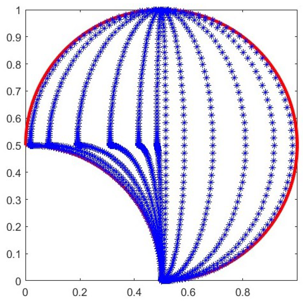
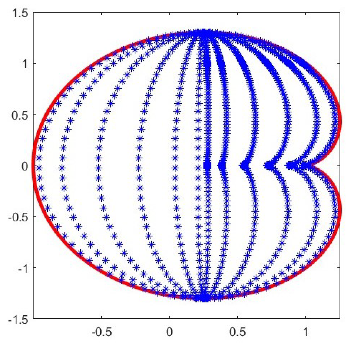
We underline that, as discussed in [
10], in general, the nodes of this cubature formula are not contained in the domain
H, but only in the minimal rectangle
with sides parallel to the axes.
However, the nodes are inside the cubature domain when there exists a straight line l such that the following property holds:
When property
holds, a change in coordinates so that
l becomes parallel to the new
y-axis implies that all the cubature nodes
are in
H, and that all the weights
are nonnegative, taking as
(which defines the nodes of the cubature formula) the intersection point of
l with the new
x-axis. For a detailed discussion on this, the interested reader can consult [
10] and the references therein.
Go back now to a general domain
, and assume that it is a compact domain whose boundary is a Jordan (simple and closed) curve, defined parametrically by two piecewise smooth functions
that are not polynomials
In [
10], it was suggested to use the Chebfun package [
12] in order to provide two piecewise polynomials
(interpolating at Chebychev–Lobatto nodes), such that
where
is the machine precision and
denotes the ordinary maximum norm on
. Denoting by
the domain whose boundary is defined as
in [
10], it was proposed to approximate
with
, and then approximate
with
.
Obviously, in order to construct the cubature for
, it is necessary that
is still a Jordan curve; that is, essentially a
simple curve. There exist sufficient conditions (see, for instance, [
11,
13]) such that is reasonable to assume that
Chebfun constructs a Jordan curve if the original boundary of
is piecewise
and a generalized regular curve, in the sense that it has no singular points and no cusps.
Concerning the convergence of the cubature rule, the following results were proven in [
10]. For any subset
of
, we denote by
the error of best polynomial approximation of the function
f by means of bivariate polynomials of total degree
m, with respect to the uniform norm on
. Moreover, let
denote the minimal rectangle containing
.
Theorem 1 ([
10], Theorem 3)
. Let Ω
be a compact domain in , whose boundary (9) is a Jordan curve, and let be the domain with the boundary, as in (11). Assume that , are at least piecewise Hölder continuous and satisfy (10). The following cubature error estimate holds for Formula (7) with where , and , in the general case, while when Ω
satisfies Property , and denotes the closed disk centered at the origin with radius . In the case when the approximated boundary is not guaranteed to be simple, as for example if the original curve has some singular points, the following error estimate holds true.
Theorem 2 ([
10], Theorem 5)
. Let Ω
be as in (9), and , be the piecewise polynomial approximating curve (10). Assume that the integrand f is Hölder-continuous with constant C and exponent on the minimal rectangle containing , where . Then, the following estimate holds for the error of the cubature formula (7) with :where . 


