Explicit Symplectic Runge–Kutta–Nyström Methods Based on Roots of Shifted Legendre Polynomial

Abstract

To date, all explicit symplectic Runge–Kutta–Nyström methods of order five or above are derived by numerical solutions of order condition equations and symplectic condition. In this paper, we derive 124 sets of seven-stage fifth-order explicit symplectic Runge–Kutta–Nyström methods with closed-form coefficients in the Butcher tableau using the roots of a degree-3 shifted Legendre polynomial. One method is analyzed and its P-stable interval is derived. Numerical tests on the two newly discovered methods are performed, showing their long-time stability and large step size stability over some existing methods.

1. Introduction

In recent decades, geometric numerical methods that preserve at least one geometric property of a given system have received significant attention in various fields, such as astrophysics, computational fluid dynamics and molecular dynamics; see monographs [1,2,3,4,5] and references therein. For other traditional numerical methods for ordinary differential equations, such as Runge–Kutta methods, we refer to the book [6].

Consider the classical second-order differential equation [2,4]

$$\ddot{q}=-▽U\left(q\right),q\left(t_0\right)=q_0,\dot{q}\left(t_0\right)=p_0,$$

where $U:{\mathbb{R}}^d\to \mathbb{R}$ is assumed to be sufficiently smooth. Introducing $p=\dot{q}$, wherein q and p are vectors, represents a function related to potential energy. An s-stage explicit symplectic Runge–Kutta–Nyström (ESRKN) method applied to the above equation is [7]

$$\begin{array}{c}\hfill \begin{array}{cc}\hfill Q_i& =q_n+h{c}_i{p}_n-h^2\sum _{j=1}^s{\overline{a}}_{ij}▽U\left(Q_j\right),\hfill \\ \hfill q_{n+1}& =q_n+h{p}_n-h^2\sum _{i=1}^s{\overline{b}}_i▽U\left(Q_i\right),\hfill \\ \hfill p_{n+1}& =p_n-h\sum _{i=1}^s{b}_i▽U\left(Q_i\right),\hfill \end{array}\end{array}$$

(1)

where h is the step size,

$$\begin{array}{c}\hfill \begin{array}{ccc}\hfill {\overline{b}}_i& =b_i(1-c_i),i=1,\dots ,s\mathrm{and}{\overline{a}}_{ij}\hfill & \hfill =\left\{\begin{array}{cc}0,\hfill & i\le j,\hfill \\ b_j(c_i-c_j),\hfill & i>j.\hfill \end{array}\right.\end{array}\end{array}$$

The ESRKN method (1) is expressed in a Butcher tableau by where the symbols match their locations in (1). For more information about Butcher tableaus, we refer to a Butcher book [6].

Therefore, an ESRKN method is determined only by nodes $c_i$ and quadrature coefficients $b_i$. There are different strategies used to obtain $c_i$ and $b_i$; we mention (without being exhaustive) the following references [5,8,9,10,11,12,13,14,15,16]. For ESRKN methods with an order higher than four, none of the aforementioned works present $c_i$ and $b_i$ in exact closed form. In other words, those methods obtained do not satisfy order conditions and symplectic conditions exactly, but within some digits of accuracy. Hence, an interesting question is whether or not there exists a closed form of $c_i$ and $b_i$ for ESRKN with an order higher than four. In this paper, we present a positive answer to this question.

In an earlier work, authors in [8] constructed a fifth-order ESRKN method by solving 13 equations of order conditions, while constructing a sixth-order method requires solving 23 equations of order conditions. Obviously, as the order increases, so does the computational cost of solving the nonlinear order equations to produce $c_i$ and $b_i$. Although the research by Calvo and Hairer has significantly reduced the number of independent order conditions in the ESRKN method [17], the coupled order conditions equations still comprise a considerable proportion of the total order conditions equations. On the other hand, despite modern computers’ tremendous performance, it is nearly impossible to solve order conditions directly to obtain $c_i$ and $b_i$ with a higher order. One possibility is to assign some suitable $c_i$ first and then solve order conditions to yield $b_i$. But what is the preassigned acceptable $c_i$? It is worth noting that the $c_i$ nodes of both three-stage fourth-order ESRKN methods in Table 1 and Table 2 are the roots of the degree-2 shifted Legendre polynomial [18].

Table 1. Scheme 1.

$\frac{1}{2}+\frac{\sqrt{3}}{6}$
$\frac{1}{2}-\frac{\sqrt{3}}{6}$	$\frac{2-\sqrt{3}}{12}$
$\frac{1}{2}+\frac{\sqrt{3}}{6}$	0	$\frac{\sqrt{3}}{6}$
ine	$\frac{5-3\sqrt{3}}{24}$	$\frac{3+\sqrt{3}}{12}$	$\frac{1+\sqrt{3}}{24}$
ine	$\frac{1}{4}-\frac{\sqrt{3}}{6}$	$\frac{1}{2}$	$\frac{1}{4}+\frac{\sqrt{3}}{6}$

Table 2. Scheme 2.

$\frac{1}{2}-\frac{\sqrt{3}}{6}$
$\frac{1}{2}+\frac{\sqrt{3}}{6}$	$\frac{2+\sqrt{3}}{12}$
$\frac{1}{2}-\frac{\sqrt{3}}{6}$	0	$-\frac{\sqrt{3}}{6}$
ine	$\frac{5+3\sqrt{3}}{24}$	$\frac{3-\sqrt{3}}{12}$	$\frac{1-\sqrt{3}}{24}$
ine	$\frac{1}{4}+\frac{\sqrt{3}}{6}$	$\frac{1}{2}$	$\frac{1}{4}-\frac{\sqrt{3}}{6}$

Numerous researchers have already successfully utilized polynomials or functions to design numerical methodologies. For instance, Revelli and Ridolfi [19] developed an interpolation collocation method based on the sine function. Additionally, a fourth-order algorithm was designed based on sinc-collocation in [20]. The successful instances have sparked a great deal of interest in our investigation for constructing higher-order ESRKN methods based on shifted Legendre polynomials.

We investigate the potential of using the degree-3 shifted Legendre polynomial roots as the $c_i$ nodes and come up with a five-stage fourth-order ESRKN method, which further confirms that it is feasible to construct ESRKN using the shifted Legendre polynomial roots as the $c_i$ nodes. We then conduct further research to derive fifth-order ESRKN methods. The main contribution of this paper is to show that this is an effective technique for deriving ESRKN methods and we demonstrate this by deriving 124 seven-stage fifth-order ESRKN methods with $c_i$ and $b_i$ in closed form. To the best of our knowledge, this is the first work carried out to derive closed-form ESRKN methods with order five. We will explore closed-form ESRKN methods with order 6 or higher in a future paper.

This paper is organized as follows. In Section 2, we introduce order conditions for the ESRKN method (1) and demonstrate two closed-form ESRKN methods with order four and five, respectively. Their P-stable intervals are also provided. Section 3 presents numerical experiments. In Section 4, some conclusions are drawn. Appendix A lists 124 sets of preassigned acceptable $c_i$, where the corresponding closed-form real solution $b_i$ could be determined by order conditions.

2. ESRKN Methods with Order 4 and 5

2.1. Order Conditions for ESRKN Method

Given the assumption ${\overline{b}}_i=b_i(1-c_i)$, the order conditions for RKN method (1) are as follows [8,21]:

$$\begin{array}{c}\hfill \begin{array}{cccc}\hfill \left(1\right)& \sum _{i=1}^s{b}_i=1,\hfill & \hfill \left(2\right)& \sum _{i=1}^s{b}_i{c}_i=\frac{1}{2},\hfill \\ \hfill \left(3\right)& \sum _{i=1}^s{b}_i{c}_i^2=\frac{1}{3},\hfill & \hfill \left(4\right)& \sum _{i=1}^s\sum _{j=1}^s{b}_i{\overline{a}}_{ij}=\frac{1}{6},\hfill \\ \hfill \left(5\right)& \sum _{i=1}^s{b}_i{c}_i^3=\frac{1}{4},\hfill & \hfill \left(6\right)& \sum _{i=1}^s\sum _{j=1}^s{b}_i{c}_i{\overline{a}}_{ij}=\frac{1}{8},\hfill \\ \hfill \left(7\right)& \sum _{i=1}^s\sum _{j=1}^s{b}_i{\overline{a}}_{ij}{c}_j=\frac{1}{24},\hfill & \hfill \left(8\right)& \sum _{i=1}^s{b}_i{c}_i^4=\frac{1}{5},\hfill \\ \hfill \left(9\right)& \sum _{i=1}^s\sum _{j=1}^s{b}_i{c}_i^2{\overline{a}}_{ij}=\frac{1}{10},\hfill & \hfill \left(10\right)& \sum _{i=1}^s\sum _{j=1}^s\sum _{k=1}^s{b}_i{\overline{a}}_{ij}{\overline{a}}_{ik}=\frac{1}{20},\hfill \\ \hfill \left(11\right)& \sum _{i=1}^s\sum _{j=1}^s{b}_i{c}_i{\overline{a}}_{ij}{c}_j=\frac{1}{30},\hfill & \hfill \left(12\right)& \sum _{i=1}^s\sum _{j=1}^s{b}_i{\overline{a}}_{ij}{c}_j^2=\frac{1}{60},\hfill \\ \hfill \left(13\right)& \sum _{i=1}^s\sum _{j=1}^s\sum _{k=1}^s{b}_i{\overline{a}}_{ij}{\overline{a}}_{jk}=\frac{1}{120}.\hfill \end{array}\end{array}$$

(2)

If only condition (1) is satisfied, the method is of order one. If both conditions (1) and (2) are satisfied, the method is of order two. If conditions (1) to (4) are satisfied, the method is of order three. If conditions (1) to (7) are satisfied, the method is of order four, and if conditions (1) to (13) are satisfied, the method is of order five. It has been demonstrated that, for ESRKN methods, conditions (7), (12) and (13) are redundant [8].

2.2. A Five-Stage Fourth-Order ESRKN Method

Let the degree-l normalized shifted Legendre polynomial $P_l\left(x\right)$ be [21],

$$P_l\left(x\right)=\frac{\sqrt{2l+1}}{l!}\frac{d^l}{d{x}^l}\left(x^l{(x-1)}^l\right),l=0,1,2,\dots .$$

The roots of degree-3 shifted Legendre polynomial $P_3\left(x\right)=\sqrt{7}(20x^3-30x^2+12x-1)$ are

$$\begin{array}{c}\hfill \begin{array}{cccccc}\hfill g_1& =\frac{1}{2}-\frac{\sqrt{15}}{10},\hfill & \hfill g_2& =\frac{1}{2},\hfill & \hfill g_3& =\frac{1}{2}+\frac{\sqrt{15}}{10}.\hfill \end{array}\end{array}$$

(3)

By placing $g_1,g_2,g_3$ in five positions as a set of $c_i$, we find a closed-form five-stage fourth-order ESRKN method whose Butcher tableau is presented in Table 3.

Table 3. Five-stage fourth-order ESRKN method.

$\frac{1}{2}+\frac{\sqrt{15}}{10}$	0	0	0	0	0
$\frac{1}{2}-\frac{\sqrt{15}}{10}$	$\frac{3}{10}-\frac{13\sqrt{15}}{180}$	0	0	0	0
$\frac{1}{2}+\frac{\sqrt{15}}{10}$	0	$\frac{\sqrt{15}}{18}$	0	0	0
$\frac{1}{2}$	$\frac{3}{20}-\frac{13\sqrt{15}}{360}$	$\frac{\sqrt{15}}{36}$	$\frac{13\sqrt{15}}{360}-\frac{3}{20}$	0	0
$\frac{1}{2}+\frac{\sqrt{15}}{10}$	0	$\frac{\sqrt{15}}{18}$	0	$\frac{2\sqrt{15}}{45}$	0
ine	$\frac{119}{360}-\frac{31\sqrt{15}}{360}$	$\frac{5}{36}+\frac{\sqrt{15}}{36}$	$\frac{31\sqrt{15}}{360}-\frac{119}{360}$	$\frac{2}{9}$	$\frac{5}{36}-\frac{\sqrt{15}}{36}$
ine	$\frac{13}{36}-\frac{\sqrt{15}}{10}$	$\frac{5}{18}$	$\frac{\sqrt{15}}{10}-\frac{13}{36}$	$\frac{4}{9}$	$\frac{5}{18}$

Theorem 1.

The explicit five-stage method defined in Table 3 is a fourth-order symplectic RKN method and its P-stable interval [22] is (0, 7.75342…).

Proof. 

It is easy to verify that parameters in Table 3 satisfy order conditions (1) to (7); therefore, it is of fourth order.

We solve the test equation $\ddot{q}=-{\lambda }^{2}q$ using the ESRKN method (1) to obtain ${\mathbf{y}}_{n+1}=M{\mathbf{y}}_n$, where

$$\begin{array}{cc}\hfill {\mathbf{y}}_n=\left(\begin{array}{c}{q}_n\\ h{\dot{q}}_n\end{array}\right),M& =\left(\begin{array}{cc}1-r{\overline{b}}^{⊺}{(I+r\overline{a})}^{-1}e& 1-r{\overline{b}}^{⊺}{(I+r\overline{a})}^{-1}c\\ -r{b}^{⊺}{(I+r\overline{a})}^{-1}e& 1-r{b}^{⊺}{(I+r\overline{a})}^{-1}c\end{array}\right).\hfill \end{array}$$

(4)

Here, $r={\lambda }^2{h}^2$, $e=\left(\begin{array}{ccc}1,& \cdots & ,1\end{array}\right)$, c, b, $\overline{b}$ and matrix $\overline{a}$ are defined in Table 3. Numerical calculations reveal that the P-stable interval is given by

$$\begin{array}{c}\hfill I_p=\{r\mid \rho \left(M\right)=1,\mathrm{tr}{\left(M\right)}^2<4det\left(M\right)\}=(0,7.75342\dots ).\end{array}$$

 □

2.3. A Seven-Stage Fifth-Order ESRKN Method

We choose the stage number as seven and place $g_1,g_2$ and $g_3$ of (3) in seven positions of $\left\{c_i\right\}$. There are $3^7=2187$ permutations for $c_i$. By solving the fifth-order conditions of 13 equations, we find real solution $b_i$ for 124 sets of $c_i$. For each set of nodes $c_i$, we present its adjoint counterpart in Appendix A. Therefore, we find in total 124 seven-stage fifth-order ESRKN methods in closed form, where $c_i$ is chosen among $g_1,g_2$ and $g_3$ of (3) and $b_i$ is solved by fifth-order conditions in (2). In particular, we display in Table 4 such an ESRKN method.

Table 4. A seven-stage fifth-order ESRKN method (cf. (5)).

$\frac{1}{2}$	0	0	0	0	0	0	0
$\frac{1}{2}-\frac{\sqrt{15}}{10}$	${\overline{a}}_{21}$	0	0	0	0	0	0
$\frac{1}{2}$	0	${\overline{a}}_{32}$	0	0	0	0	0
$\frac{1}{2}-\frac{\sqrt{15}}{10}$	${\overline{a}}_{41}$	0	${\overline{a}}_{43}$	0	0	0	0
$\frac{1}{2}+\frac{\sqrt{15}}{10}$	${\overline{a}}_{51}$	${\overline{a}}_{52}$	${\overline{a}}_{53}$	${\overline{a}}_{54}$	0	0	0
$\frac{1}{2}-\frac{\sqrt{15}}{10}$	${\overline{a}}_{61}$	0	${\overline{a}}_{63}$	0	$-\frac{\sqrt{15}}{18}$	0	0
$\frac{1}{2}$	0	${\overline{a}}_{72}$	0	${\overline{a}}_{74}$	$-\frac{\sqrt{15}}{36}$	$-\frac{1}{20}$+$\frac{\sqrt{15}}{72}$	0
ine	${\overline{b}}_1$	${\overline{b}}_2$	${\overline{b}}_3$	${\overline{b}}_4$	$\frac{5}{36}-\frac{\sqrt{15}}{36}$	$\frac{7}{360}-\frac{\sqrt{15}}{360}$	$\frac{1}{9}-\frac{\sqrt{15}}{30}$
ine	$b_1$	$b_2$	$b_3$	$b_4$	$\frac{5}{18}$	$\frac{5}{36}-\frac{\sqrt{15}}{30}$	$\frac{2}{9}-\frac{\sqrt{15}}{15}$

Here, in Table 4,

$$\begin{array}{c}\hfill \begin{array}{cc}\hfill b_1& =-\frac{137\sqrt{15}}{1296}+\frac{1}{2}-\frac{\sqrt{21955335-5576400\sqrt{15}}}{6480},\hfill \\ \hfill b_2& =\frac{1117\sqrt{15}}{6480}-\frac{5}{18}-\frac{\sqrt{21955335-5576400\sqrt{15}}}{6480},\hfill \\ \hfill b_3& =\frac{1117\sqrt{15}}{6480}-\frac{5}{18}+\frac{\sqrt{21955335-5576400\sqrt{15}}}{6480},\hfill \\ \hfill b_4& =-\frac{901\sqrt{15}}{6480}+\frac{5}{12}+\frac{\sqrt{21955335-5576400\sqrt{15}}}{6480},\hfill \\ \hfill {\overline{b}}_i& =b_i(1-c_i)\mathrm{and}{\overline{a}}_{ij}=b_j(c_i-c_j).\hfill \end{array}\end{array}$$

(5)

Theorem 2.

The seven-stage explicit method defined in Table 4 is a fifth-order symplectic RKN method and its P-stable interval is (0, 9.22575…).

Proof. 

We verify the 13 equations in (2) by plugging the coefficients $c_i$, $b_i$, ${\overline{b}}_i$ and ${\overline{a}}_{ij}$ from Table 4. We compute the spectrum of M in (4) with c, b, $\overline{b}$ and $\overline{a}$ from Table 4 to obtain

$$\begin{array}{c}\hfill I_p=\{r\mid \rho \left(M\right)=1,\mathrm{tr}{\left(M\right)}^2<4det\left(M\right)\}=(0,9.22575\dots ).\end{array}$$

 □

3. Numerical Experiments

We compute two numerical examples. The first example has a known solution that the computation verifies, determining the symplecticity-preserving and the order convergence of the new methods. The second example shows a strong stability of the new methods over some existing methods.

We solve the Kepler problem, cf. [4],

$$\begin{array}{cc}\hfill \ddot{\mathbf{q}}& =f\left(\mathbf{q}\right),f(\left(\begin{array}{c}{q}_1\\ q_2\end{array}\right))=\left(\begin{array}{c}-q_1/{(q_1^2+q_2^2)}^{3/2}\\ -q_2/{(q_1^2+q_2^2)}^{3/2}\end{array}\right),\hfill \\ \hfill \mathbf{q}\left(0\right)& =\left(\begin{array}{c}4\\ 0\end{array}\right),\dot{\mathbf{q}}\left(0\right)=\left(\begin{array}{c}0\\ \sqrt{13/40}\end{array}\right).\hfill \end{array}$$

The Hamiltonian is

$$\begin{array}{cc}\hfill H(\mathbf{q},\dot{\mathbf{q}})& =\frac{{\dot{q}}_1^2+{\dot{q}}_2^2}{2}-\frac{1}{{(q_1^2+q_2^2)}^{1/2}}.\hfill \end{array}$$

(6)

The exact solution is

$$\begin{array}{cc}\hfill q_1\left(t\right)& =\frac{cos\left(E\right(t\left)\right)-e}{1-e}·4,q_2\left(t\right)=T(1-e)sin\left(E\left(t\right)\right)\sqrt{13/40},\hfill \end{array}$$

where $e=3/10$, $T=2\pi a^{3/2}$, $a=40/7$ and $E\left(t\right)$ is the solution of the Kepler equation

$$\begin{array}{c}\hfill E\left(t\right)-esin\left(E\left(t\right)\right)=a^{-3/2}t.\end{array}$$

We solve the Kepler problem in $t\in [0,5T]$ using the five-stage fourth-order method defined in Table 3, and using the seven-stage fifth-order method defined in Table 4, with grid size $h=5T/2^7$, …, $5T/2^{12}$. In Figure 1, we plot the error of the computed Hamiltonian (6). It indicates that both methods are symplectic. The error is roughly caused by the computer round-off.

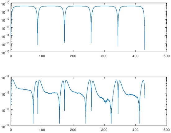
Figure 1. The error of computed Hamiltonian, $H(\mathbf{q},\dot{\mathbf{q}})-H({\mathbf{q}}_0,{\dot{\mathbf{q}}}_0)$, on $[0,5T]$, using the five-stage fourth-order method (top) and using the seven-stage fifth-order method (bottom).

In Table 5, we list the computed error at $t=5T$ and the computed order of convergence using the fifth-stage fourth-order method in Table 3, and using the seven-stage fifth-order method defined in Table 4.

Table 5. Error profile using the 5-stage 4th order method in Table 3 (left), and using the 7-stage 5th order method in Table 4 (right).

h	$|{\mathit{q}}_1\left(5\mathit{T}\right)-{\mathit{q}}_1^{\mathit{N}}|$	Order	$|{\mathit{q}}_2\left(5\mathit{T}\right)-{\mathit{q}}_2^{\mathit{N}}|$	Order
$5T/2^7$	1.832 × 10${}^{-1}$	—	7.271 × 10${}^{-3}$	—
$5T/2^8$	1.251 × 10${}^{-2}$	3.9	1.293 × 10${}^{-4}$	5.8
$5T/2^9$	8.009 × 10${}^{-4}$	4.0	2.091 × 10${}^{-6}$	6.0
$5T/2^{10}$	5.035 × 10${}^{-5}$	4.0	3.296 × 10${}^{-8}$	6.0
$5T/2^{11}$	3.152 × 10${}^{-6}$	4.0	5.140 × 10${}^{-10}$	6.0
$5T/2^{12}$	1.971 × 10${}^{-7}$	4.0	4.690 × 10${}^{-12}$	6.8

We next solve the Hénon–Heiles Hamiltonian system [23,24]

$$\begin{array}{c}\hfill \begin{array}{cc}\hfill & {\dot{p}}_1=-q_1-2q_1{q}_2,{\dot{q}}_1=p_1,\hfill \\ \hfill & {\dot{p}}_2=-q_2-q_1^2+q_2^2,{\dot{q}}_2=p_2,\hfill \end{array}\end{array}$$

(7)

with initial values $(p_1,p_2,q_1,q_2)=(0,0,0.1,-0.5)$. The corresponding Hamiltonian function is denoted by

$$H(p,q)=\frac{1}{2}(p_1^2+p_2^2)+\frac{1}{2}(q_1^2+q_2^2)+q_1^2{q}_2-\frac{1}{3}{q}_2^2.$$

(8)

In the following experiments, we apply four ESRKN methods to (7): the five-stage fourth-order ESRKN method listed in Table 3; the seven-stage fifth-order ESRKN method listed in Table 4; the five-stage fifth-order ESRKN method from [8] listed in the first part of Table 6, which satisfies the order condition with an error tolerance of ${10}^{-15}$; the seven-stage fifth-order RKN method from [10] listed in the second part of Table 6, which satisfies the order condition with an error tolerance of less than 3 × ${10}^{-16}$. In short, we will denote these four methods as NEW4, NEW5, OS5 and CS5, cf. the abbreviation table at the end. In all the following figures, the cyan, red, magenta and blue lines denote the results derived by NEW4, NEW5, OS5 [8] and CS5 [10], respectively.

Table 6. Top: the five-stage fifth-order method (OS5) from [8]. Bottom: the seven-stage fifth-order method (CS5) from [10].

$c_1$	0.69883375727544694289	$b_1$	0.40090379269664777606
$c_2$	0.20413810365459889029	$b_2$	$0.95997088013412390506$
$c_3$	1.02055757000418534370	$b_3$	$0.08849515812721633901$
$c_4$	0.36292800323075291580	$b_4$	$1.22143909234910252870$
$c_5$	0.30508610893167564804	$b_5$	$-1.67080892330709041000$
$c_1$	0.0000000000000000	$b_1$	$0.06281213570268329$
$c_2$	0.2179621390175646	$b_2$	$0.37889831312525750$
$c_3$	0.4424703708255242	$b_3$	$0.27545285152613400$
$c_4$	1.4784605594388980	$b_4$	$-0.001585299574780513$
$c_5$	0.3400000000000000	$b_5$	$-0.17857040385276180$
$c_6$	0.7000000000000000	$b_6$	$0.34799958341988310$
$c_7$	1.0000000000000000	$b_7$	$0.11499281965358440$

In Table 7, we present the convergence rates of the NEW4, NEW5, OS5 [8] and CS5 [10] methods, where global errors for q and p corresponding to these four methods at five step sizes h in the time interval [0, 1] are provided. It verifies the convergence rates of all four methods.

Table 7. Convergence rates for NEW4, NEW5, OS5 [8] and CS5 [10] methods at $t=1$.

h	NEW4		NEW5		OS5 [8]		CS5 [10]
	Error	Order	Error	Order	Error	Order	Error	Order
$2^{-2}$	1.2779 × 10${}^{-5}$	—	2.7640 × 10${}^{-6}$	—	4.6273 × 10${}^{-5}$	—	2.3635 × 10${}^{-7}$	—
$2^{-3}$	7.7886 × 10${}^{-7}$	4.04	8.0660 × 10${}^{-8}$	5.10	1.2286 × 10${}^{-6}$	5.23	7.3171 × 10${}^{-9}$	5.01
$2^{-4}$	4.8164 × 10${}^{-8}$	4.02	2.4460 × 10${}^{-9}$	5.04	3.5467 × 10${}^{-8}$	5.11	2.2908 × 10${}^{-10}$	4.99
$2^{-5}$	2.9957 × 10${}^{-9}$	4.00	7.5375 × 10${}^{-11}$	5.01	1.0657 × 10${}^{-9}$	5.05	7.1838 × 10${}^{-12}$	5.00
$2^{-6}$	1.8680 × 10${}^{-10}$	4.00	2.3438 × 10${}^{-12}$	5.00	3.2652 × 10${}^{-11}$	5.03	2.3228 × 10${}^{-13}$	4.95

The research findings from [25] revealed that particles of (7) manifest chaotic behavior when the system energy $H>\frac{1}{12}$. Furthermore, it was proposed that when H is less than $\frac{1}{6}$, particle trajectories are confined within the equilateral triangle defined by $H=\frac{1}{6}$. For the sake of this study, an initial value of $H=\frac{1}{6}$ is selected, resulting in chaotic numerical behavior while constraining trajectories within the triangular region. This property is expected to be retained by symplectic numerical methods. Numerical computations have demonstrated, however, that those methods such as OS5 [8] and CS5 [10], which do not fully meet the order condition equations and symplectic condition, are incapable of retaining long-term stability. After a certain time, the variations in particle trajectories escalate rapidly, eventually exceeding the boundaries of the triangular region.

Figure 2 illustrates the trajectory plots derived from numerical simulations of the Hénon–Heiles system within the interval [0, 1000] using a step size of $h=0.5$. All four methods display trajectories that are confined within the equilateral triangle area in this situation. Nonetheless, Figure 3 shows that when the OS5 [8] method is used to generate numerical trajectories within the interval [0, 17,575], the trajectories escape directly from the upper region. Figure 4 looks into the causes of the OS5 [8] method’s escape phenomena, attributing them to the numerical inability to maintain system energy. The capacity of symplectic algorithms to maintain correct numerical behavior over lengthy periods of time is a significant advantage. Therefore, we continue to increase the time interval. In Figure 5, it is evident that the NEW4, NEW5 and CS5 [10] methods maintain accurate numerical behavior even at t = 100,000.

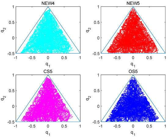
Figure 2. Solving the numerical orbit diagram of the Hénon–Heiles system over the interval [0, 1000] with a step size of $h=0.5$.

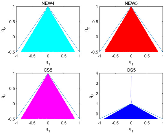
Figure 3. Solving the numerical orbit diagram of the Hénon–Heiles system over the interval [0, 17,575] with a step size of $h=0.5$.

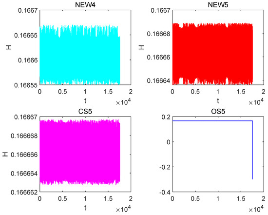
Figure 4. Computing the Hamiltonian energy diagram of the Hénon–Heiles system over the interval [0, 17,575] with a step size of $h=0.5$.

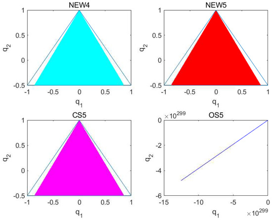
Figure 5. Solving the numerical orbit diagram of the Hénon–Heiles system over the interval [0, 100,000] with a step size of $h=0.5$.

With such extensive time intervals, the need for further comparisons with bigger time intervals appears to be decreasing for the NEW4, NEW5 and CS5 [10] methods. As a result, the step size is steadily increased in the interval [0, 10,000], beginning with $h=0.50$ and gradually increasing until it reaches $h=0.86$. The CS5 [10] method begins to gradually deviate from the triangular region at this point. However, the NEW4 and NEW5 methods continue to display reliable numerical performance in the face of such variances. These phenomena are illustrated in Figure 6. Finally, Figure 7 depicts the variation in Hamiltonian energy over time using the NEW4, NEW5 and CS5 [10] methods, emphasizing that the inability to maintain system energy is the cause of the escape phenomena.

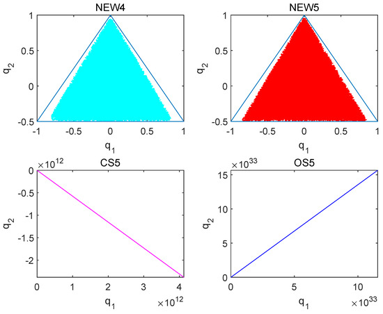
Figure 6. Solving the numerical orbit diagram of the Hénon–Heiles system over the interval [0, 10,000] with a step size of $h=0.86$.

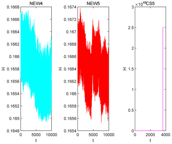
Figure 7. Computing the Hamiltonian energy diagram of the Hénon–Heiles system over the interval [0, 10,000] with a step size of $h=0.86$.

4. Discussion

This article introduces an approach to constructing ESRKN methods that precisely satisfy the order conditions and the symplectic conditions, resulting in 124 sets of seven-stage fifth-order ESRKN methods. Based on the results of numerical experiments, it is clear that using ESRKN methods that exactly meeting the order conditions and the symplectic conditions has advantages over approaches that have inherent errors in satisfying these criteria. In light of these findings, a future research will be dedicated to developing sixth-order ESRKN methods.

References

- Leimkuhler, B.; Reich, S. Simulating Hamiltonian Dynamics; Cambridge Monographs on Applied and Computational Mathematics; Cambridge University Press: Cambridge, UK, 2004; Volume 14. [Google Scholar] [CrossRef]
- Hairer, E.; Lubich, C.; Wanner, G. Geometric Numerical Integration: Structure-Preserving Algorithms for Ordinary Differential Equations, 2nd ed.; Springer Series in Computational Mathematics; Springer: Berlin/Heidelberg, Germany, 2006; Volume 31. [Google Scholar] [CrossRef]
- Feng, K.; Qin, M. Symplectic Geometric Algorithms for Hamiltonian Systems; Springer: Berlin/Heidelberg, Germany, 2010; Volume 449. [Google Scholar]
- Blanes, S.; Casas, F. A Concise Introduction to Geometric Numerical Integration; Monographs and Research Notes in Mathematics; CRC Press: Boca Raton, FL, USA, 2016. [Google Scholar] [CrossRef]
- Sanz-Serna, J.; Calvo, M. Numerical Hamiltonian Problems; Courier Dover Publications: New York, NY, USA, 2018. [Google Scholar]
- Butcher, J. The Numerical Analysis of Ordinary Differential Equations. Runge–Kutta and General Linear Methods; Wiley: Hoboken, NJ, USA, 1987. [Google Scholar]
- Okunbor, D.; Skeel, R. Explicit canonical methods for Hamiltonian systems. Math. Comput. 1992, 59, 439–455. [Google Scholar] [CrossRef]
- Okunbor, D.; Skeel, R. Canonical Runge-Kutta-Nyström methods of orders five and six. J. Comput. Appl. Math. 1994, 51, 375–382. [Google Scholar] [CrossRef]
- Tsitouras, C. A tenth-order symplectic Runge-Kutta-Nyström method. Celest. Mech. Dyn. Astron. 1999, 74, 223–230. [Google Scholar] [CrossRef]
- Chou, L.; Sharp, P. On order 5 symplectic explicit Runge-Kutta-Nyström methods. J. Appl. Math. Decis. Sci. 2000, 4, 143–150. [Google Scholar] [CrossRef]
- Xiao, A.; Tang, Y. Order properties of symplectic Runge-Kutta-Nyström methods. Comput. Math. Appl. 2004, 47, 569–582. [Google Scholar] [CrossRef]
- Franco, J.; Gómez, I. Some procedures for the construction of high-order exponentially fitted Runge-Kutta-Nyström methods of explicit type. Comput. Phys. Commun. 2013, 184, 1310–1321. [Google Scholar] [CrossRef]
- Wang, B.; Wu, X. A highly accurate explicit symplectic ERKN method for multi-frequency and multidimensional oscillatory Hamiltonian systems. Numer. Algorithms 2014, 65, 705–721. [Google Scholar] [CrossRef]
- Blanes, S.; Casas, F.; Escorihuela-Tomàs, A. Runge-Kutta-Nyström symplectic splitting methods of order 8. Appl. Numer. Math. 2022, 182, 14–27. [Google Scholar] [CrossRef]
- Kovalnogov, V.; Fedorov, R.; Karpukhina, M.; Kornilova, M.; Simos, T.; Tsitouras, C. Runge-Kutta-Nyström methods of eighth order for addressing linear inhomogeneous problems. J. Comput. Appl. Math. 2023, 419, 12. [Google Scholar] [CrossRef]
- Yang, H.; Zeng, X. The tri-coloured free-tree theory for symplectic multi-frequency ERKN methods. J. Comput. Appl. Math. 2023, 423, 20. [Google Scholar] [CrossRef]
- Calvo, M.; Hairer, E. Further reduction in the number of independent order conditions for symplectic, explicit partitioned Runge-Kutta and Runge-Kutta-Nyström methods. Appl. Numer. Math. 1995, 18, 107–114. [Google Scholar] [CrossRef]
- Qin, M.; Zhu, W. Canonical Runge-Kutta-Nyström (RKN) methods for second order ordinary differential equations. Comput. Math. Appl. 1991, 22, 85–95. [Google Scholar] [CrossRef]
- Revelli, R.; Ridolfi, L. Sinc collocation-interpolation method for the simulation of nonlinear waves. Comput. Math. Appl. 2003, 46, 1443–1453. [Google Scholar] [CrossRef]
- Yang, X.; Wu, L.; Zhang, H. A space-time spectral order sinc-collocation method for the fourth-order nonlocal heat model arising in viscoelasticity. Appl. Math. Comput. 2023, 457, 128192. [Google Scholar] [CrossRef]
- Tang, W.; Zhang, J. Symplecticity-preserving continuous-stage Runge-Kutta-Nyström methods. Appl. Math. Comput. 2018, 323, 204–219. [Google Scholar] [CrossRef]
- Franco, J. Stability of explicit ARKN methods for perturbed oscillators. J. Comput. Appl. Math. 2005, 173, 389–396. [Google Scholar] [CrossRef]
- Hénon, M.; Heiles, C. The applicability of the third integral of motion: Some numerical experiments. Astron. J. 1964, 69, 73–79. [Google Scholar] [CrossRef]
- Hénon, M. Numerical exploration of Hamiltonian Systems. In Chaotic Behaviour of Deterministic Systems; Iooss, G., Ed.; Elsevier Science Ltd.: Amsterdam, The Netherlands, 1983; pp. 53–170. [Google Scholar]
- Feng, K. K. Feng’s Collection of Works; National Defence Industry Press: Beijing, China, 1995; Volume 2. [Google Scholar]
Disclaimer/Publisher’s Note: The statements, opinions and data contained in all publications are solely those of the individual author(s) and contributor(s) and not of MDPI and/or the editor(s). MDPI and/or the editor(s) disclaim responsibility for any injury to people or property resulting from any ideas, methods, instructions or products referred to in the content. |
© 2023 by the authors. Licensee MDPI, Basel, Switzerland. This article is an open access article distributed under the terms and conditions of the Creative Commons Attribution (CC BY) license (https://creativecommons.org/licenses/by/4.0/).