Asymptotic Results of Some Conditional Nonparametric Functional Parameters in High-Dimensional Associated Data

Abstract

In this paper, we propose to study the asymptotic properties of some conditional functional parameters, such as the distribution function, the density, and the hazard function, for an explanatory variable with values in a Hilbert space (infinite dimension) and a response variable real in a quasi-associated dependency framework. We consider the non parametric estimation of the conditional distribution function by the kernel method in the presence of the quasi-associated dependence, and we establish under general hypotheses the almost complete convergence with speed of the estimator built in the associated case. The estimation of the conditional hazard function will be conducted by utilizing the two outcomes of the conditional distribution function and the conditional density. We establish the asymptotic normality of the kernel estimator as the conditional risk function of a properly normalized functional. We explicitly give the asymptotic variance. Simulation studies were conducted to investigate the behavior of the asymptotic property in the context of finite sample data. All the statistical analyses were performed using R software.

1. Introduction

Mathematics and statistical analysis techniques have been of considerable relevance in a variety of scientific sectors in recent years, including engineering, economics, clinical medicine, and healthcare. In particular, the application of methods of mathematical and statistical analysis have been applied to engineering, economics, healthcare, and clinical medicine, and is has been demonstrated how these approaches may assist in such vital areas as comprehension, prediction, correlation, diagnosis, therapy, and data processing.

It is crucial to note that the study of conditional models, which is included in nonparametric functional data analysis, is one of the most significant approaches of statistical analysis. An examination of this kind is carried out with the primary purpose of investigating and modeling the connection that exists between a scalar response variable and a functional regressor. In addition, two essential asymptotic features are the consistency and the asymptotic normality of particular statistical parameter estimators.

Functional data are the subject of this research. As defined in Ref. [1], statistics functional data analysis (FDA) analyzes infinite-dimensional variables, including curves, sets, and pictures. The “Big Data” revolution has spurred its rapid expansion over the past 20 years.

This may be demonstrated by researching the topic’s past (for an example, see [2]). In [3], the topics of density and mode estimation for normed vector space data and the problem of excessive dimensionality in functional data and are discussed and potential remedies are offered. Nonparametric models were investigated for use in regression estimation in [4].

The treatment of functional data today typically involves contemporary theory. For example, reference [5] presented the consistency rates of a variety of conditional distribution functionals, such as the regression function, conditional cumulative distribution, and conditional density, uniformly over a subset of the explanatory variable. These functionals include the conditional cumulative distribution and conditional density. The conditional cumulative distribution, as well as the conditional density, are both included in these functionals.

Uniformly in bandwidth (UIB) consistency was extended to the ergodic scenario, and the rates of consistency for different functional nonparametric models were investigated in [6]. The regression function was a part of these models, a conditional hazard function, conditional distribution, and conditional density.

In the field of statistical mathematics, in recent years, there has been a surge of curiosity in the statistical analysis of functional data. These numbers are used in econometrics, medicine, environmental science, and many other fields. In the statistical functional, ref. [4] made the first attempt to estimate the conditional density function and its derivatives. In addition, they were the ones who were the first to do so in the scientific community. These authors reached an extent of convergence in the i.i.d. case that was really near to being finished. Since this work was published, much more research has been done on estimating the conditional density and its derivatives, especially for computing the conditional mode. In point of fact, ref. [7] demonstrated that a kernel estimator of the conditional mode will almost certainly converge to the true value. The authors showed this by taking into account data that included a-mixing.

The point that nullifies the kernel density estimator derivative was used by [8,9] to estimate the conditional mode. This was done to determine the conditional mode. The outcomes were comparable using this approach, but they put more of an emphasis on the estimator’s asymptotic normality, which was provided in both the i.i.d and mixed circumstances, respectively. Both scenarios included mixing. Ref. [10] was able to identify the level of accuracy of the terms that dominate the quadratic error that is produced by the kernel density estimator.

We suggest that the reader check [11] for further information on the smoothing parameter that should be used in estimating the conditional density in relation to the functional explanatory variable.

The concept of a quasi-association variable refers to a variable that exhibits some degree of association with another variable; examples of research that processed data under both positive and negative dependent random variables are [12,13,14]. In Ref. [15], the authors were the first people to offer the concept of quasi-association to conduct an analysis of real-valued stochastic occurrences. This is a very striking illustration of the idea of weak reliance. It was used by [16] for real-valued random fields, and it provides a unified technique for studying families of positively dependent and negatively dependent random variable families.

According to our knowledge, the nonparametric estimation of quasi-associated random variables is addressed in a vanishingly small number of published papers. The study conducted by [17] focuses on a limit theorem for quasi-associated Hilbertian random variables. The research conducted by [18] explores asymptotic results for an M-estimator of the regression for weak dependance; and in Ref. [19], the authors investigated both quasi-associated processes and asymptotic results. Ref. [20] investigated the asymptotic normality of this final estimator as part of the study, which focused on the single-index structure of the conditional hazard function.

To solve relative regression, ref. [21] explored the nonparametric estimate for linked random variables; it was found to be significant in [22,23]. Both of these results were found to be significant. The authors were responsible for conducting these investigations in their own separate ways. The authors in [24] demonstrate the robust uniform consistency characteristics of partial derivatives of multivariate density functions under weak dependence, namely inside compact subsets of $R_d$, and they determine the relevant rates of convergence to establish the asymptotic normality of these estimators.

In [25], the authors examine the application of the kernel nearest neighbors (k-nn) technique in a regression model with a single index. They specifically focus on cases where the explanatory variable is measured in functional space, in the context of the association dependency condition. The primary outcome of this study involves the determination of the asymptotic distribution for the single index estimator using the k-nn.

The study conducted in [26] examines the application of the k-nn approach within the single index regression model. This particular investigation focuses on scenarios where the predictor is functional in nature, and the response is scalar. The primary outcome of this study is the determination of the almost comprehensive rates of convergence under the assumption of weak dependence.

The primary outcome of the study referenced in [27] is the establishment of the asymptotic properties, specifically the almost complete convergence rates and the asymptotic normality, of nonparametric estimation techniques for the regression function in the context of the single functional index model (SFIM). These features are derived under the assumption of quasi-association dependence.

It is important to keep in mind that our results are connected to the model’s functional space in some manner, just as they are related to every previous asymptotic statistics functional nonparametric finding.

In this research, we establish under general hypotheses the almost complete convergence with the speed of the estimator built in the quasi-associated case, and we will apply the two results of the conditional distribution function and the conditional density in [28] to estimate the conditional hazard function. We establish the asymptotic normality of the kernel estimator as the conditional hazard function of a properly normalized functional. We give explicitly the asymptotic variance.

In the subsequent sections of this work, we will introduce our model, which can be found in Section 2. In Section 3 of this paper, the primary findings are presented. The confidence bands is the subject of discussion in Section 4. In Section 5, an analysis and evaluation of the behavior of our asymptotic normality findings on finite sample data is conducted. The conclusion is articulated in Section 6. The proof of the intermediate findings is provided in Appendix A.

2. Model and Estimator

To commence, we provide a precise delineation of quasi-association about random variables that possess values within a separable Hilbert space.

Consider a separable Hilbert space $(\mathcal{H},<.,.>)$ furnished with an orthonormal basis. The sequence of elements is represented by $e_k,k\ge 1$.

Let ${\left(R_n\right)}_{n\in \mathbb{N}}$ be a sequence of real random variables with values in $\mathcal{H}$. The statement is made that this sequence exhibits quasi-association about the basis. The user defines $e_k$ as a variable. The term “quasi-associated” is used to describe the sequence $e_k$ if, for any positive integer d, the d-dimensional sequence $\{(<R_i,e_{j1}>,\dots ,<R_i,e_{jd}>),i\in \mathbb{N}\}$ is also quasi-associated.

In this analysis, we will examine a group of n quasi-associated random variables, which we will represent as $W_i={(R_i,S_i)}_{1\le i\le n}$. The random variables mentioned exhibit the same distribution as the random variable $W=(R,S)$, which represents values in a separable real Hilbert space denoted as $\mathcal{H}\times \mathbb{R}$. This Hilbert space is equipped with an inner product denoted as $<.,.>$, which generates the norm. The semi-metric d is considered, as given by: $\forall r,r^{\prime }\in \mathcal{H}/d(r,r^{\prime })=\parallel r-r^{\prime }\parallel$.

For a fixed r in the $\mathcal{H}$ space, its fixed neighborhood ${\mathcal{N}}_r$ and a compact subset of $\mathbf{R}$ all have the notation $\mathcal{S}$. For each $r\in {\mathcal{N}}_r$, there is a S such that $R=r$. Using a sample of n dependent observations from $W:=(R,S)$, the conditional distribution function $F^r\left(s\right)$ is estimated. We present the $\widehat{F}{}^r\left(s\right)$ estimator of $F^r\left(s\right)$, a kernel type estimator, defined as:

$$\widehat{F}{}^r\left(s\right)=\frac{{\sum }_{i=1}^{n}K\left(h_H^{-1}d(r,R_i)\right)H\left(h_H^{-1}(s-S_i)\right)}{K\left(h_H^{-1}d(r,R_i)\right)},\forall s\in \mathbb{R}$$

(1)

K: denotes the kernel, H represents a particular distribution function, and the sequence of positive real integers $h_K=h_{K,n}$ (resp. $h_H=h_{H,n}$) converges to zero when n increases to infinity. We define $\widehat{f}{}^r\left(s\right)$ estimator of the conditional density $f^r\left(s\right)$, given by:

$${\displaystyle \widehat{f}{}^r\left(s\right)=\frac{{\displaystyle h_H^{-1}\sum _{i=1}^{n}K\left(h_K^{-1}d(r,R_i)\right)H^{\prime }\left(h_H^{-1}(s-S_i)\right)}}{{\displaystyle \sum _{i=1}^{n}K\left(h_K^{-1}d(r,R_i)\right)}},\forall s\in \mathbb{R}.}$$

(2)

This is the derivative of H expressed as $H^{\prime }$.

Finally, we obtain the conditional hazard function estimator $\widehat{Z}{}^r\left(s\right)$. This estimator is defined as follows:

$$\widehat{Z}{}^r\left(s\right)=\frac{\widehat{f}{}^r\left(s\right)}{1-\widehat{F}{}^r\left(s\right)},\forall s\in \mathbb{R}.$$

(3)

3. The Consistency and Asymptotic Normality of the Kernel Estimators

3.1. Assumptions and Necessary Background Knowledge

When there is no chance of misunderstanding, we shall designate any strictly positive generic constants in the paper by the notation l or/and $l^{{}^{\prime }}$. This will only happen when there is no risk of mistakes. The expression w in the process signifies a fixed point in $\mathcal{H}$, and ${\mathcal{N}}_w$ stands for a fixed neighborhood of w. We take into account the fact that the random couple $\{(W_i,T_i),i\in \mathcal{N}\}$ is a process that is stationary.

Let ${\lambda }_k$ denote the covariance coefficient, which may be found by using the equation:

$${\lambda }_k=su{p}_{s\ge k}\sum _{|i-j|\ge s}{\lambda }_{i,j}$$

(4)

In

$${\lambda }_{i,j}=\sum _{k=1}^{\infty }\sum _{l=1}^{\infty }|Cov(W_i^k,W_j^l)|+\sum _{k=1}^{\infty }|Cov(W_i^k,T_j)|+\sum _{l=1}^{\infty }|Cov(W_i,X_j^l)|+|Cov(T_i,T_j)|$$

The $k\mathrm{th}$ component of $W_i$, as represented by $R_i^k$, where $R_i^k:=<W_i,e^k>$ is the definition of $R_i^k$. Let us denote the ball as $B(w,h):=\{r^{\prime }\in \mathcal{H}/d(w^{\prime },w)<h\}$. This represents the ball with a center of w and a radius $h,$ when $h>0$.

For the purpose of establishing the virtually full convergence of the estimator of $\widehat{F}{}^r\left(s\right)$. In order to establish the results of our research, it will be necessary to rely on the following assumptions.

(P1)

$\mathbb{P}(R\in B(r,h))={\varphi }_r\left(h\right)>0$ and the function ${\varphi }_r\left(h\right)$ is a differentiable at 0.

There exists a function $\beta (r,.)$ such that:

$${\displaystyle \forall s^{{}^{\prime }}\in [0,1],\underset{h\to 0}{lim}\frac{{\varphi }_r\left(s^{{}^{\prime }}{h}_K\right)}{{\varphi }_r\left(h_K\right)}=\beta (r,s^{{}^{\prime }})}$$

(P2)

The conditional distribution function $F^r\left(s\right)$ satisfies the Holder condition, that is: $\forall (r_1,r_2)\in {\mathcal{N}}_r\times {\mathcal{N}}_x,\forall (s_1,s_2)\in {\mathcal{S}}^2$

$$|f^{r_1}\left(s_1\right)-f^{r_2}\left(s_2\right)|⩽l\left(d^{z_1}(r_1,r_2)+{|s_1-s_2|}^{z_2}\right)z_1>0,z_2>0$$

$$|F^{r_1}\left(s_1\right)-F^{r_2}\left(s_2\right)|⩽l\left(d^{z_3}(r_1,r_2)+{|s_1-s_2|}^{z_4}\right)z_3>0,z_4>0$$

Here, $\mathcal{S}$ is a fixed compact subset of $\mathbb{R}$.

(P3)

The kernel, denoted by H, is a differentiable function, and its inverse, denoted by $H^{\prime }$, is a positive, bounded, and Lipschitzian continuous function:

$${\int \left|t\right|}^{z_2}{H}^{\prime }\left(t\right)dt<\infty and\int H^{\prime 2}\left(t\right)dt<\infty$$

(P4)

For K, we have the necessary conditions for it to be a bounded continuous Lipschitz function, which are:

$${l\Vert }_{[0,1]}(.)<K(.)<l^{{}^{\prime }}{\Vert }_{[0,1]}(.)$$

Here, ${\Vert }_{[0,1]}$ is referred to as an indicator function.

(P5)

A quasi-association exists between the sequence of random pairings $(R_i,S_i)$, where $i\in \mathcal{N}$, and the covariance coefficient ${\lambda }_k,k\in \mathcal{N}$, as long as the conditions are met.

$$\exists a>0,\exists l>0,then{\lambda }_k\le l{e}^{-ak}$$

(P6)

The joint distribution functions are defined so that they hold for each and every pair $(i,j)$.

$${\Psi }_{i,j}\left(h\right)=\mathbb{P}[(R_i,R_j)\in B(r,h)\times B(r,h))]$$

satisfy:

$$\underset{i\ne j}{sup}{\Psi }_{i,j}\left(h\right)=O\left({\varphi }_r^2\left(h_k\right)\right)>0$$

(P7)

The frequencies $(h_K,h_H)$, verified:

(i)${\displaystyle \underset{n\to \infty }{lim}{h}_K=0,}$ ${\displaystyle \underset{n\to \infty }{lim}{h}_H=0}$

(ii)${\displaystyle \underset{n\to \infty }{lim}(h_H^{b_2}+h_K^{b_1})\sqrt{n{h}_H{\varphi }_r\left(h_K\right)}=0}$

(iii) ${lim}_{n\to \infty }\frac{{log}^5\left(n\right)}{n{h}_H^j{\varphi }_r\left(h_k\right)}=0$ for $j=0\mathrm{and}j=1$

3.2. Brief Comment on the Conditions

The attribute of concentration of the explanatory variable is denoted by the Assumption (P1) in the context of tiny balls. The function $\beta (r,.)$ is very important to any asymptotic study, but especially for the variance term. The inclusion of Condition (P2) in our model serves the purpose of regulating the smoothness of the functional space. The inclusion of these components is important in order to accurately calculate the bias component of the convergence rates. The (P3) and (P4) Assumptions, similarly, center on the cumulative function H and its associated kernels $K^{\prime }{H}^{\prime }$ and K. The word “bias” is purposefully left out of the asymptotic normalcy result thanks to this assumption. The presumption (P5) represents a normative restriction on the quasi-associated information. Our model is assumed to be asymptotically normal under quasi-association if and only if the joint distribution of the pair ($R_i,R_j$) follows the assumptions of assumption (P6). This will enable us to demonstrate that our model exhibits asymptotic normality. Adopting assumption (P7) is required to rule out the possibility of “bias” in the final result of asymptotic normalcy, and this assumption is well-known as a classical one in functional estimation in spaces of finite or infinite dimensions.

3.3. Almost Complete Convergence of $\widehat{F}{}^r\left(s\right)$

Theorem 1.

Based on assumptions (P1)–(P7), we have:

$$|\widehat{F}{}^r\left(s\right)-F^r\left(s\right)|=O(h_K^{b1}+h_K^{b2})+O\left({\left(\frac{Log\left(n\right)}{n{\varphi }_r\left(h_K\right)}\right)}^{\frac{1}{2}}\right)$$

(5)

Proof of Theorem 1.

The subsequent decomposition, together with the lemmas that are listed below, provide the foundation for the proof:

$$\begin{array}{cc}\hfill \widehat{F}{}^r\left(s\right)-F^r\left(s\right)& =\frac{1}{\widehat{F}{}_D^r}\left(\left(\widehat{F}{}_N^r\left(s\right)-\mathbb{E}\widehat{F}{}_N^r\left(s\right)\right)-\left(F^r\left(s\right)-\mathbb{E}\widehat{F}{}_N^r\left(s\right)\right)\right)\hfill \\ \hfill & +\frac{F^r\left(s\right)}{\widehat{F}{}_D^r}\left(\widehat{F}{}_D^r-\mathbb{E}\widehat{F}{}_D^r\right)\hfill \end{array}$$

(6)

where

$$\widehat{F}{}_N^r\left(s\right)=\frac{1}{n\mathbb{E}\left[K_1\left(r\right)\right]}\sum _{i=1}^n{K}_i\left(r\right)H_i\left(s\right)$$

and

$$\widehat{F}{}_D^r=\frac{1}{n\mathbb{E}\left[K_1\left(r\right)\right]}\sum _{i=1}^n{K}_i\left(r\right)$$

with

$$K_i\left(r\right)=K\left(h_K^{-1}d(r,R_i)\right)and{H}_i\left(s\right)=H\left(h_H^{-1}(s-S_i)\right)$$

Lemma 1.

Based on assumptions (P1)–(P4) and (P6):

$$\frac{1}{\widehat{F}{}_D^r\left(s\right)}\left(\widehat{F}{}_N^r\left(s\right)-E\widehat{F}{}_N^r\left(s\right)\right)=O_{a.co}\left({\left(\frac{Log\left(n\right)}{n{\varphi }_R\left(h_K\right)}\right)}^{\frac{1}{2}}\right)$$

(7)

Corollary 1.

Based on assumptions (P1)–(P4) and (P6), we have:

$$\sum _{i=1}^{\infty }\mathbb{P}\left(|\widehat{F}{}_D^r\left(s\right)|<1/2\right)<\infty$$

(8)

Lemma 2.

Based on assumptions (P1)–(P6), we have:

$$\frac{1}{\widehat{F}{}_D^r\left(s\right)}\left(F^r\left(s\right)-E\widehat{F}{}_N^r\left(s\right)\right)=O(h_K^{b1}+h_K^{b2})$$

(9)

Lemma 3.

Based on assumptions (P1)–(P7), we have:

$$\widehat{F}{}_D^r\left(s\right)-E\widehat{F}{}_D^r\left(s\right)=O_{a.co}\left({\left(\frac{log\left(n\right)}{n{\varphi }_r\left(h_K\right)}\right)}^{\frac{1}{2}}\right)$$

(10)

□

Theorem 1 may be derived from these lemmas, where their proofs appear in Appendix A.

3.4. Almost Complete Convergence of $\widehat{Z}{}^r\left(s\right)$

Theorem 2.

Based on assumptions (P1)–(P7), we have:

$$|\widehat{Z}{}^r\left(s\right)-Z^r\left(s\right)|=O\left(h_K^{b_1}+h_K^{b_2}\right)+O_{a.co}\left({\left(\frac{logn}{n{h}_H{\varphi }_r\left(h_K\right)}\right)}^{\frac{1}{2}}\right).$$

(11)

Proof of Theorem 2.

The basis for this analysis is derived from the subsequent decomposition.

$$\widehat{Z}{}^r\left(s\right)-Z^r\left(s\right)=\frac{1}{1-\widehat{F}{}^r\left(s\right)}\left[\widehat{f}{}^r\left(s\right)-f^r\left(s\right)\right]+\frac{h^r\left(s\right)}{1-\widehat{F}{}^r\left(s\right)}\left[\widehat{F}{}^r\left(s\right)-F^r\left(s\right)\right]$$

(12)

and therefore asymptotic results for the estimator $\widehat{Z}{}^r\left(s\right)$ can be readily deduced from $\widehat{F}{}^r\left(s\right)$ and $\widehat{f}{}^r\left(s\right)$.

After the decomposition precedent, all you have to do demonstrate:

Lemma 4

(See proof of Theorem 1). Based on assumptions (P1)–(P7), we obtain:

$$\left|\widehat{F}{}^r\left(s\right)-F^r\left(s\right)\right|=O\left(h_K^{b_1}+h_K^{b_2}\right)+O_{a.co}\left({\left(\frac{logn}{n{\varphi }_r\left(h_K\right)}\right)}^{\frac{1}{2}}\right)$$

(13)

Lemma 5

(See Bouaker et al. (2021) [28]). Based on assumptions (P1)–(P7), we obtain:

$$\left|\widehat{f}{}^r\left(s\right)-f^r\left(s\right)\right|=O\left(h_K^{b_1}+h_K^{b_2}\right)+O_{a.co}\left({\left(\frac{logn}{n{h}_H{\varphi }_r\left(h_K\right)}\right)}^{\frac{1}{2}}\right)$$

(14)

Corollary 2.

Based on assumptions (P1)–(P7), we obtain:

$$\exists \delta >0,\sum _{i=1}^{\infty }\mathbb{P}\left\{\left(1-\widehat{F}{}^r\left(s\right)\right)<\delta \right\}<\infty .$$

(15)

□

3.5. Asymptotic Normality of the Conditional Hazard Function Estimate

Theorem 3.

Based on the assumptions, we obtain, for any $r\in \mathcal{A}$:

$$\sqrt{n{h}_H{\varphi }_r\left(h_K\right)}\left(\widehat{Z}{}^r\left(s\right)-Z^r\left(s\right)\right)\stackrel{\mathcal{D}}{⟶}\mathcal{N}(0,{\sigma }_h^2\left(r\right))asn\to \infty$$

(16)

where

$$\mathcal{A}=\{r\in \mathcal{H},f^r\left(s\right)(1-F^r\left(s\right))\ne 0\}$$

and

$${\displaystyle {\sigma }_h^2\left(r\right)=\frac{C_2{Z}^r\left(s\right)}{C_1^2(1-F(s,r))}\int H^{\prime 2}\left(t\right)dt,}$$

In

$${\displaystyle C_j=K\left(1\right)-{\int }_0^1{\left(K^j\right)}^{\prime }\left(s\right)\beta (r,s)ds,forj=1,2.}$$

The symbol $\stackrel{\mathcal{D}}{⟶}$ denotes convergence in distribution.

Proof of Theorem 3.

The basis for this analysis is derived from the subsequent decomposition.

$$\begin{array}{c}\hfill \widehat{Z}{}^r\left(s\right)-Z^r\left(s\right)=\frac{1}{\widehat{F}{}_D^r-\widehat{F}{}_N^r\left(s\right)}\left[\widehat{f}{}_N^r\left(s\right)-f^r\left(s\right)\right]-\frac{Z^r\left(s\right)}{\widehat{F}{}_D^r-\widehat{F}{}_N^r\left(s\right)}\left[\widehat{F}{}_D^r-\widehat{F}{}_N^r\left(s\right)+F^r\left(s\right)-1\right]\end{array}$$

(17)

where

$$\widehat{f}{}_N^r\left(s\right)=\frac{1}{n{h}_H\mathbb{E}\left[K_1\left(r\right)\right]}\sum _{i=1}^n{K}_i\left(r\right)H_i^{\prime }\left(s\right).$$

Lemma 6.

Based on assumptions (P1)–(P7), we have:

$$\begin{array}{c}\hfill \sqrt{n{h}_H{\varphi }_r\left(h_K\right)}\left(\widehat{f}{}_N(s,r)-\mathbb{E}\left(\widehat{f}{}_N(s,r)\right)\right)\stackrel{\mathcal{D}}{\to }\mathcal{N}\left(0,{\sigma }_f^2\left(r\right)\right),n\to \infty \end{array}$$

(18)

where

$$\begin{array}{c}\hfill {\sigma }_f^2\left(r\right)=\frac{C_{2}f(s,r)}{C_1^2}\int H^2\left(t\right)dt\end{array}$$

Lemma 7.

(See Daoudi, H. and Mechab, B. (2019) [22]). Under assumptions (P1)–(P5); we have:

$$\begin{array}{c}\hfill \mathbb{E}\left(\widehat{f}{}_N^r\left(s\right)\right)-f^r\left(s\right)=O\left(h_H^{b_2}\right)+O\left(h_K^{b_1}\right),n\to \infty \end{array}$$

(19)

Lemma 8.

Based on assumptions (P1)–(P7), we have:

$$\begin{array}{c}\hfill \sqrt{n{h}_H{\varphi }_r\left(h_K\right)}\left[\widehat{F}{}_D^r-\widehat{F}{}_N^r\left(s\right)+F^r\left(s\right)-1\right]\to 0 in probability, n\to \infty \end{array}$$

(20)

Corollary 3.

Based on assumptions (P1)–(P7), we have:

$$\begin{array}{c}\hfill \left[\widehat{F}{}_D^r-\widehat{F}{}_N^r\left(s\right)\right]\to 1-F^r\left(s\right) in probability\end{array}$$

(21)

□

4. Confidence Bands

One important aspect in statistical analysis is the establishment of confidence bands for estimations. These confidence bands provide a range of values within which we can be confident that the true value lies. By calculating and interpreting these confidence bands, we can gain a better understanding of the uncertainty associated with our estimations. The objective of this section create confidence intervals for the actual value of $Z^r\left(s\right)$ for a specified curve with the format $<R,R{}^{\prime }>=<r,r{}^{\prime }>$. Estimation using nonparametric methods relies on the asymptotic variance, which is determined by a number of unknown functions. Regarding our situation, we have:

$${\displaystyle {\sigma }_Z^2\left(r\right)=\frac{C_2{Z}^r\left(s\right)}{C_1^2(1-F^r\left(s\right))}}$$

(22)

The variables $Z^r\left(s\right),F^r\left(s\right),C_1$, and $C_2$ are not known in advance and must be approximated during the practical implementation. It is possible to derive confidence bands even when ${\sigma }_Z^2\left(r\right)$ is functionally given. An estimate for $\widehat{\sigma }{}_Z^2\left(r\right)$ may be produced using $\widehat{Z}{}^{\left(r\right)}\left(s\right)$, $\widehat{F}{}^{\left(r\right)}\left(s\right)$, ${\widehat{C}}_1$, and ${\widehat{C}}_2$ for $Z^{\left(r\right)}\left(s\right)$, $F^{\left(r\right)}\left(s\right)$, $C_1$, and $C_2$, respectively.

$${\displaystyle \widehat{\sigma }{}_Z^2\left(r\right)=\frac{\widehat{C}{}_2\widehat{Z}{}^r\left(s\right)}{\widehat{C}{}_1^2(1-\widehat{F}{}^r\left(s\right))}.}$$

(23)

The constants $C_1$ and $C_2$ are estimated empirically in the following manner:

$${\displaystyle \widehat{C}{}_1=\frac{1}{n{\varphi }_r\left(h_K\right)}\sum _{i=1}^{n}K\left(h_K^{-1}d(r,R_i)\right),\widehat{C}{}_2=\frac{1}{n{\varphi }_r\left(h_K\right)}\sum _{i=1}^n{K}^2\left(h_K^{-1}d(r,R_i)\right)}$$

where

$${\displaystyle {\varphi }_r\left(h_K\right)=\frac{1}{n}\sum _{i=1}^n{\mathbb{I}}_{\left\{\right|<r-R_i>|<h_K\}}.}$$

The expression for the asymptotic confidence band at a significance level of $1-\zeta$ for $Z^r\left(s\right)$ is provided as follows.

$$\left[\widehat{Z}{}^r\left(s\right)-u_{1-\frac{\zeta }{2}}{\left({\displaystyle \frac{\widehat{\sigma }{}_Z^2\left(r\right)}{n{\varphi }_r\left(h_K\right)}}\right)}^{1/2},\widehat{Z}{}^r\left(s\right)+u_{1-\frac{\zeta }{2}}{\left({\displaystyle \frac{\widehat{\sigma }{}_Z^2\left(r\right)}{n{\varphi }_r\left(h_K\right)}}\right)}^{1/2}\right]$$

where $u_{1-\frac{\zeta }{2}}$ denotes the $1-\frac{\zeta }{2}$ quantile of the standard normal distribution.

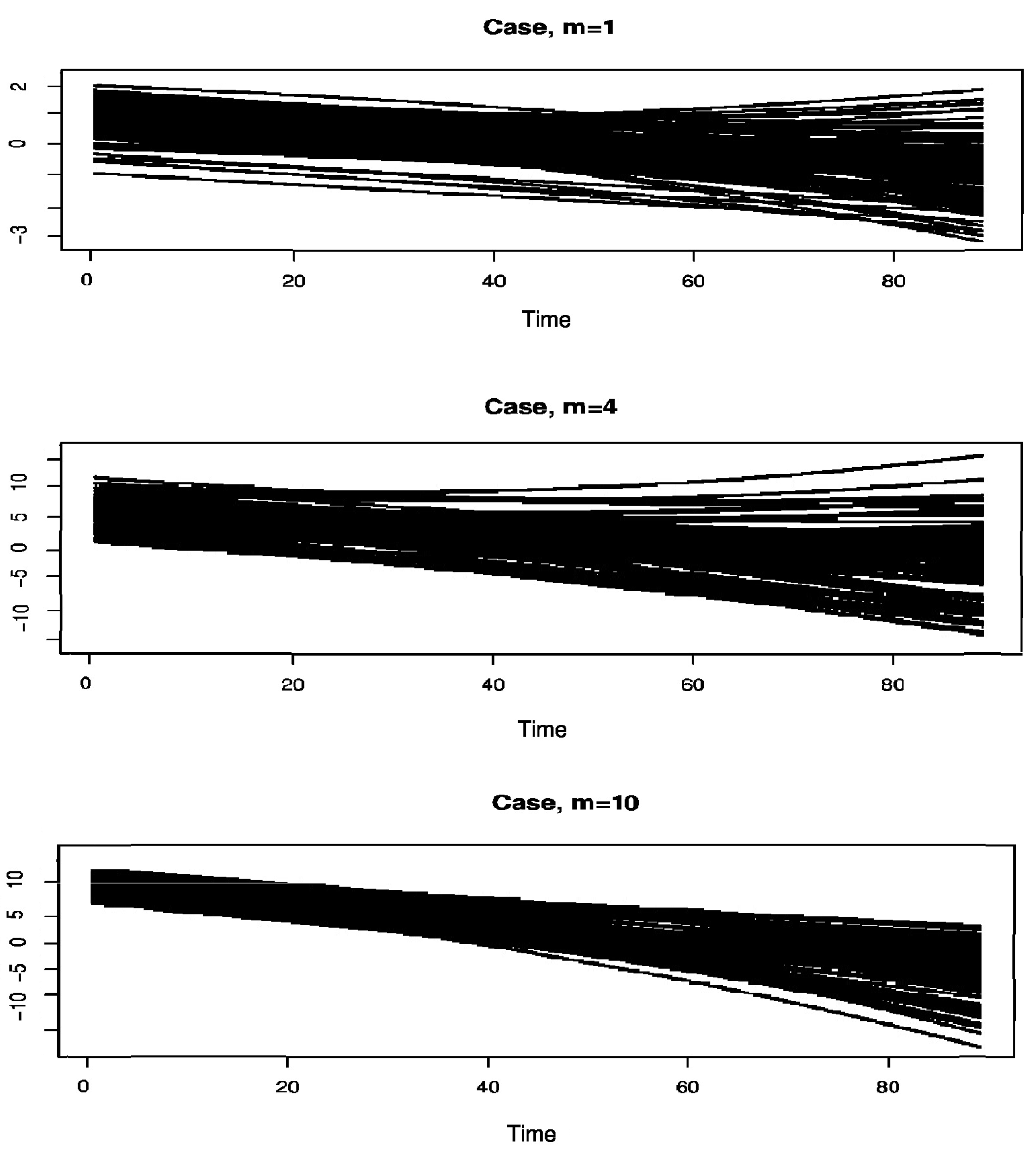
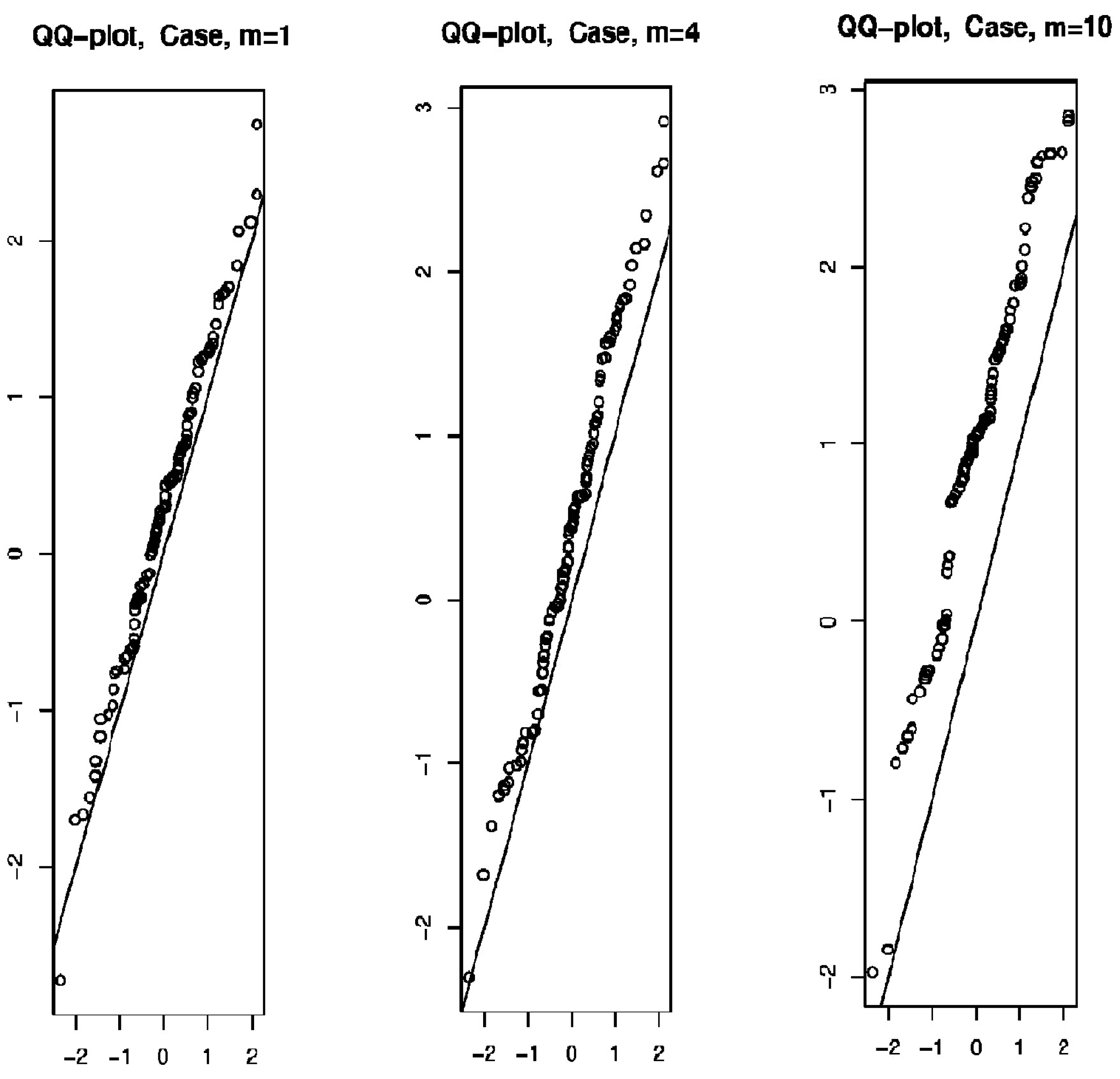
5. A Simulation Study

Within this particular section, we examine how our asymptotic normality conclusions behave across data from a limited sample. Our primary purpose is to demonstrate how simple the conditional risk function is to develop and to study the effect of dependency on this asymptotic characteristic.

We produce functional observations for this purpose by investigating the functional nonparametric model that is shown below:

$$Z_i=r\left(W_i\right)+{ϵ}_i\mathrm{for}i=1,\dots ,n$$

(24)

where ${ϵ}_i⇝\mathcal{N}(0,.5).$

The linear process with quasi-associated variables is well known to satisfy requirement ($P6$). As a result, the functional regressor with quasi-associates shown below is constructed.

$$Z_i\left(t\right)=\sum _{j=i+1}^{i+m}{\Gamma }_j\left(t\right)$$

(25)

where

$${\Gamma }_j\left(t\right)=s_j{t}^2+h_j\ast t+g_{j}t\in [0,1]$$

$${\left(s_j\right)}_j⇝\mathcal{N}(0,\frac{1}{2})(\mathrm{resp}.{\left(h_j\right)}_j⇝\mathcal{N}(-1,\frac{1}{2})\mathrm{and}{\left(g_j\right)}_j⇝\mathcal{N}(1,\frac{1}{2})).$$

Figure 1 shows the $Z_i$’s curves discretized in the same 100-point grid in [0, 1] for m = 1, 4, and 10 values. Furthermore, the regression operator computes the scalar variable $Z_i$:

$$r\left(w\right)=5{\int }_0^{1}exp\left\{W\left(t\right)\right\}dt.$$

(26)

It can be seen that, by examining the error distribution (${ϵ}_i$), we are able to infer the theoretical conditional distribution function of Z given $W=w$. This function is explicitly determined by shifting the distribution of (${ϵ}_i$) by $r\left(w\right)$. Therefore, the determination of the theoretical distribution of the conditional hazard function may be easily determined.

To demonstrate this function’s asymptotic normality, we fix one curve, $w=W_0$, and $z=Z_0$, from the created data, then collect m independent n-samples of the same data and compute the quantity:

$$\sqrt{n{h}_H{\varphi }_{(}r,h_K)}\widehat{\sigma }{}_{h_K}^{-1}\left(r\right)\left(\widehat{Z}{}^r\left(s\right)-Z^r\left(s\right)\right)$$

(27)

where ${\widehat{\sigma }}_{h_K}$ is the previous section’s standard deviation estimation.

The collected sample is next tested for normality. With the cross-validation approach determined, we utilized a quadratic kernel, represented as:

$$K\left(t\right)=\frac{3}{2}(1-t^2){\mathbb{I}}_{[0,1]}.$$

Figure 2 depicts a graph of the collected sample versus a typical normal distribution at varied m = 1, 4, and 10 values.

The performance of our estimator demonstrates its favorable characteristics and reliable performance in practical applications. Furthermore, the correlation of the data has a significant impact on the pace at which the asymptotic normality converges to its final state. Specifically, its magnitude diminishes in proportion to the values of m.

Table 1. The p-value indicated by the test of Kolmogorov–Smirnov.

m	1	4	10
p-value	0.88	0.67	0.43

summarizes the p-value from the Kolmogorov–Smirnov test for each value of m, which confirms an inverse relationship between the correlation of the data and the convergence rate of the asymptotic normality.

6. Conclusions and Perspectives

The current study examines the asymptotic properties of certain conditional functional parameters, specifically the distribution function, density, and hazard function. These parameters are analyzed in the context of an explanatory variable that takes values in a Hilbert space of infinite dimension and a response variable that is real in a quasi-associated dependency framework. The estimators’ asymptotic characteristics, including practically certain convergence and normality, are derived in this study using standard conditions that encompass the key components of the research, such as the functional related assumption and the nonparametric nature of the model. The computational aspect highlights the significance of this estimator in practical applications due to its efficiency in updating findings with each new piece of information. Furthermore, the current contribution also presents intriguing avenues for further exploration. It would be of interest to establish the asymptotic normality of the estimators we have proposed in order to generalize the findings to incomplete data, such as missing, censored, or shortened data. One potential trajectory for future research involves the exploration of more intricate dependence structures, such as the ergodic spatial dependence.

References

1. Aneiros, G.; Cao, R.; Fraiman, R.; Genest, C.; Vieu, P. Recent advances in functional data analysis and high-dimensional statistics. Multivar. Anal. 2019, 170, 3–9. [Google Scholar] [CrossRef]
2. Araujo, A.; Giné, E. The Central Limit Theorem for Real and Banach Valued Random Variables; Wiley Series in Probability and Mathematical Statistics; John Wiley and Sons: New York, NY, USA; Chichester, UK; Brisbane, Australia, 1980; p. xiv+233. [Google Scholar]
3. Gasser, T.; Hall, P.; Presnell, B. Nonparametric estimation of the mode of a distribution of random curves. J. R. Stat. Society. Ser. B 1998, 60, 681–691. [Google Scholar] [CrossRef]
4. Ferraty, F.; Vieu, P. Nonparametric Functional Data Analysis: Theory and Practice; Springer Series in Statistics; Springer: New York, NY, USA, 2006. [Google Scholar]
5. Ferraty, F.; Laksaci, A.; Tadj, A.; Vieu, P. Rate of uniform consistency for nonparametric estimates with functional variables. J. Stat. Plan. Inference 2010, 140, 335–352. [Google Scholar] [CrossRef]
6. Kara-Zaitri, L.; Laksaci, A.; Rachdi, M.; Vieu, P. Uniform in bandwidth consistency for various kernel estimators involving functional data. J. Non Parametr. Stat. 2017, 29, 85–107. [Google Scholar] [CrossRef]
7. Ferraty, F.; Peuch, A.; Vieu, P. Modèle à indice fonctionnel simple. Comptes Rendus Math. 2003, 336, 1025–1028. [Google Scholar] [CrossRef]
8. Ezzahrioui, M.; Ould-Saïd, E. Asymptotic Results of a Nonparametric Conditional Quantile Estimator for Functional Time Series. Commun. Stat. Theory Methods 2008, 37, 2735–2759. [Google Scholar] [CrossRef]
9. Ezzahrioui, M.; Ould-Said, E. On the asymptotic properties of a nonparametric estimator of the conditional mode for functional dependent data. J. Nonparametr. Stat. 2008, 20, 3–18. [Google Scholar] [CrossRef]
10. Laksaci, A. Convergence en moyenne quadratique de l’estimateur à noyau de la densité conditionnelle avec variable explicative fonctionnelle. Ann. L’Institut Stat. L’Université Paris 2007, 51, 69–80. [Google Scholar]
11. Laksaci, A.; Maref, F. Estimation non paramétrique de quantiles conditionnels pour des variables fonctionnelles spatialement dépendantes. Comptes Rendus Math. 2009, 347, 1075–1080. [Google Scholar] [CrossRef]
12. Matula, P. A note on the almost sure convergence of sums of negatively dependent random variables. Stat. Probab. Lett. 1992, 15, 209–213. [Google Scholar] [CrossRef]
13. Newman, C.M. Asymptotic independence and limit theorems for positivelyand negatively dependent random variables: In Inequalities in Statistics and Probability. IMS Lect. Notes Monogr. Ser. 1984, 5, 127–140. [Google Scholar]
14. Roussas, G.G. Positive and negative dependence with some statistical applications. In Asymptotics, Nonparametrics and Time Series; Ghosh, S., Ed.; Marcell Dekker, Inc.: New York, NY, USA, 1999; pp. 757–788. [Google Scholar]
15. Doukhan, P.; Louhichi, S. A new weak dependence condition andapplications to moment inequalities. Stoch. Process. Their Appl. 1999, 84, 313–342. [Google Scholar] [CrossRef]
16. Bulinski, A.; Suquet, C. Normal approximation for quasi-associated random fields. Stat. Probab. Lett. 2001, 54, 215–226. [Google Scholar] [CrossRef]
17. Douge, L. Théorèmes limites pour des variables quasi-associées hilbertiennes. Ann. L’Institut Stat. L’Université Paris 2010, 54, 51–60. [Google Scholar]
18. Attaoui, S.; Laksaci, A.; Ould-Said, E. Asymptotic Results for an M-estimator of the Regression Function for Quasi-Associated Processes. In Functional Statistics and Applications. Contributions to Statistics; Springer International Publishing: Cham, Switzerland, 2015; pp. 3–28. [Google Scholar] [CrossRef]
19. Tabti, H.; Ait Saïdi, A. Estimation and simulation of conditionalhazard function in the quasi-associated framework when the observationsare linked via a functional single-index structure, Commun. Stat. Theory Methods 2017, 47, 816–838. [Google Scholar]
20. Hamza, D.; Mechab, B.; Chikr Elmezouar, Z. Asymptotic normality of a conditional hazard function estimate in the single index for quasi-associated data. Commun. Stat. Theory Methods 2020, 49, 513–530. [Google Scholar] [CrossRef]
21. Laksaci, A.; Mechab, W. Nonparametric relative regression for associatedrandom variables. Metron 2016, 74, 75–97. [Google Scholar]
22. Daoudi, H.; Mechab, B. Asymptotic Normality of the Kernel Estimate of Conditional Distribution Function for the quasi-associated data. Pak. J. Stat. Oper. Res. 2019, 15, 999–1015. [Google Scholar]
23. Daoudi, H.; Mechab, B.; Benaissa, S.; Rabhi, A. Asymptotic normality of the nonparametric conditional density function esti-mate with functional variables for the quasi-associated data. Int. J. Stat. Econ. 2019, 20, 94–106. [Google Scholar]
24. Allaoui, S.; Bouzebda, S.; Chesneau, C.; Liu, J. Uniform almost sure convergence and asymptotic distribution of the wavelet-based estimators of partial derivatives of multivariate density function under weak dependence. J. Nonparametr. Stat. 2021, 33, 170–196. [Google Scholar] [CrossRef]
25. Mohammedi, M.; Bouzebda, S.; Laksaci, A.; Bouanani, O. Asymptotic normality of the k-NN single index regression estimator for functional weak dependence data. Commun. Stat. Theory Methods 2022, 33, 1–26. [Google Scholar] [CrossRef]
26. Bouzebda, S.; Laksaci, A.; Mohammedi, M. The k-nearest neighbors method in single index regression model for functional quasi-associated time series data. Rev. Mat. Complut. 2023, 36, 361–391. [Google Scholar] [CrossRef]
27. Bouzebda, S.; Laksaci, A.; Mohammedi, M. Single Index Regression Model for Functional Quasi-Associated Times Series Data. REVSTAT Stat. J. 2023, 20, 605–631. [Google Scholar]
28. Bouaker, I.; Belguerna, A.; Daoudi, H. The consistency of the kernel estimation of the Function conditional density for associated Data in high-dimensional statistics. J. Sci. Arts 2022, 22, 247–256. [Google Scholar] [CrossRef]
29. Kallabis, R.S.; Neumann, M.H. An exponential inequality under weakdependence. Bernoulli 2006, 12, 333–350. [Google Scholar] [CrossRef]
30. Doob, J.L. Stochastic Processes; John Wiley and Sons: New York, NY, USA, 1953. [Google Scholar]
Figure 1. A sample of 200 curves.
Mathematics 11 04290 g001
Figure 2. The QQ-plot of the obtained sample.
Mathematics 11 04290 g002