Radio Number for Friendship Communication Networks

Abstract

This paper investigates the radio labeling of friendship networks ($F_{3,k},F_{4,k},F_{5,k}$, and $F_{6,k}$). In contrast, a mathematical model is proposed for determining the upper bound of radio numbers for ($F_{3,k},F_{4,k},F_{5,k}$, and $F_{6,k}$). A computational investigation is presented to demonstrate that our results are superior to those of the past. In conclusion, the empirical study demonstrates that the proposed results surpass the previous ones in terms of the upper bound of the radio number and the run-time.

1. Introduction

Wireless communication includes all techniques and methods of connecting and communicating between devices using a wireless signal and wireless communication technologies and gadgets. Wireless communication network services may appear in many areas, such as satellite communications, internet technology, mobile telephony, military communications, TV and radio broadcasting, and many others. Rapid development in wireless communication services led to a depletion of the most important resources and frequencies in the radio spectrum. Such development affects the economic cost of available frequencies. The reusing of frequencies may give good economies, but on the other hand, it may decrease the quality of the communication service. Using the same frequencies for many wireless communication networks leads to unacceptable interference among signals. This motivated the frequency assignment problem (FAP). Given a set of transmitters in a network, the main procedure of FAP is the assignment of frequencies to transmitters, keeping interference at an acceptable level, and making use of the available frequencies in an efficient way. Such constraints of interference are related to the use of the same (or almost the same) frequencies for transmitters within a certain range from each other. The smaller the distance is among transmitters, the stronger the interference is that occurs. Therefore, it is suggested that the difference in frequency assignments should be greater.

The graph theory introduces an effective model for this problem. The interference between transmitters is modeled as a graph, and this graph is called an interference graph $G(V,E)$. Every vertex from $V\left(G\right)$ stands for a unique transmitter. Any two vertices are adjacent (connected by an edge) if and only if the broadcasting of their corresponding transmitters may interfere. The frequency channels are labeled by positive integers. Hence, the vertex coloring (labeling) problem of the graph $G$ with some constraints on the labeling is equivalent to FAP [1], where it is shown that the propagation of the signal may lead to interference in regions with a large distance from each other. As a result, not only must nearby transmitters be assigned different frequencies but they should be effectively separated. This results in the modeling of FAP as distance-constrained labeling of the graph $G.$ For some services, it is adequate that the transmitters should have distinct frequencies; moreover, the nearby transmitters inquired to use channels with appropriate separation. In this situation, FAP is equivalent to the radio labeling problem of the graph $G$ (see ref. [2]). The radio labeling problem of graph $G$ is described as follows. Let $G=\left(V\left(G\right),E\left(G\right)\right)$ be a connected graph. For any $u,v\in V\left(G\right)$, let $d\left(u,v\right)$ denote the distance between two vertices $u,v$. That is $d\left(u,v\right)$ stands for the length of the shortest path between $u,v.$ The maximum distance between any two vertices in $G$ is defined as the diameter of $G$ and denoted as $diam\left(G\right)$. Thus, $diam\left(G\right)=\mathit{max}\left\{d\left(u,v\right):u,v\in V\left(G\right)\right\}$. A radio labeling of $G$ is a one-to-one mapping $L$ from $V\left(G\right)$ to $N$, where $N$ is the set of natural number, satisfying the condition

$$\left|L\left(u\right)-L\left(v\right)\right|\ge diam\left(G\right)+1-d\left(u,v\right).\mathit{For}\mathit{all}u,v\in V\left(G\right).$$

The span of a labeling $L$ is the maximum integer (span) that $L$ assigns to a vertex in $G$. The main objective of the radio labeling problem is to find the minimum span over all such labeling $L$ of the graph $G$. Such minimum span is denoted as $rn\left(G\right)$ or the radio number of $G.$ Saha [3] introduced an algorithm that determines the lower and upper bounds of the radio number of a graph. Badr and Moussa [4] proposed the development of Saha’s algorithm and introduced a novel mathematical model for the radio labeling application. The radio labeling problem has been studied for different families of graphs [5,6,7,8,9,10,11,12,13,14,15,16,17,18]. For more details about the mathematical models, the reader can refer to [19,20,21,22,23,24,25,26,27,28,29,30].

As the number of wireless networks and services increase, this leads to many transmission stations that may be close to each other. Consequently, in most cases, there is at least one transmission station that will overlap with many other stations. This inhibits the ability of the receiver to decipher incoming signals. This concept is illustrated in Figure 1, which shows a typical situation in which the signal of transmission stations A and B overlap in the vicinity of transmission station C as in Figure 1a, while Figure 1b shows the modeling of this interference by path graph. Whenever the number of transmission stations increases, as Figure 2a, every station hopes to increase its coverage area, which leads to more physical overlapping and hence, more radio frequency interference. This situation can be modeled by the friendship graph as shown in Figure 2b.

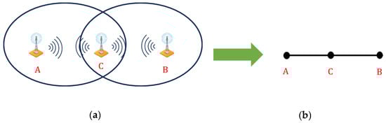
Figure 1. Path graph for modeling frequency interference of stations A, B and C. (a) Physical frequency interference. (b) Path interference graph.

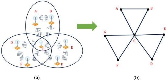
Figure 2. Friendship graph for modeling frequency interference of stations A, B, C, D, E, F and G. (a) Many transmitting stations and more Physical frequency interference. (b) Friendship interference graph.

The objective of the present paper is to study the radio labeling of friendship networks ($F_{3,k},F_{4,k},F_{5,k}$, and $F_{6,k}$). On the other hand, a mathematical model is proposed to find the upper bound of $F_{3,k},F_{4,k},F_{5,k},$ and $F_{6,k}.$ A computational study is presented to prove the efficiency of our results compared to the previous results. Finally, the empirical study shows that the proposed results outperform the previous results according to the upper bound of the radio number and the running time.

The rest of this paper is organized as follows. Section 2 presents the upper bounds for the radio number of the above-mentioned friendship graphs. The integer linear programming model of radio labeling of such friendship graphs is presented in Section 3. In Section 4, we present an experimental study for comparing results obtained in Section 2 and Section 3, and algorithms that solved the same problem from [3,4]. The conclusion of this paper and future work are presented in Section 5.

2. Radio Number of Friendship Graph

In this section, we seek to find the upper bound of $rn\left(G\right)$ where $G$ is a friendship graph.

Definition 1.

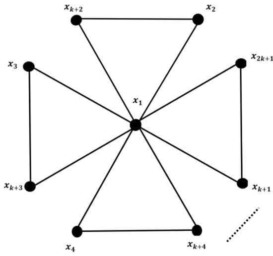
For the given positive integers $k,m$, a friendship graph, denoted as $F_{m,k}$, is represented as $k$ cycles (blocks), each of length $m$, and all have one common vertex. For an illustration, $F_{3,k}$ is shown in Figure 3.

Figure 3. $F_{3,k}$ with labeling of vertices.

Definition 2.

The order of the graph $G$ is the cardinality of its vertex set $V\left(G\right).$

Theorem 1.

The radio number of the friendship graph $F_{3,k}$ is its order.

Proof. 

Following Definition 1 for $F_{3,k}$, we find that $diam\left(F_{3,k}\right)=2$, $\left|V\left(F_{3,k}\right)\right|=2k+1,$ and $d\left(x_i{,x}_j\right)\ge 1$ for any $x_i,x_j\in V\left(F_{3,k}\right)$ and $i\ne j$. Since any radio labeling $L$ is one-to-one, it follows that

$$rn\left(F_{3,k}\right)\ge \left|V\left(F_{3,k}\right)\right|$$

(1)

Define the map $L$ with codomain $\left\{\mathrm{0,2},3,\cdots ,2k+1\right\}$ as follows:

$$\begin{gathered} L\left(x_1\right)=0; \\ L\left(x_i\right)=i;2\le i\le 2k+1 \end{gathered}$$

Now, we claim to prove that $\left|L\left(x_i\right)-L\left(x_j\right)\right|\ge diam\left(F_{3,k}\right)+1-d\left(x_i{,x}_j\right)$, that is

$$\left|L\left(x_i\right)-L\left(x_j\right)\right|\ge 3-d\left(x_i{, x}_j\right)\mathrm{for}\mathrm{all}{x}_i,x_j\in V\left(F_{3,k}\right)\mathrm{and}i\ne j.$$

Case 1. Let $2\le i\le k+1$ and $2\le j\le k+1.$ Then, $\left|L\left(x_i\right)-L\left(x_j\right)\right|=\left|i-j\right|\ge 1.$

Since $d\left(x_i{,x}_j\right)=2,$ then, $\left|L\left(x_i\right)-L\left(x_j\right)\right|\ge 3-d\left(x_i{,x}_j\right).$

Case 2. Let $i=1,j\in \left\{\mathrm{2,3},\cdots ,2k+1\right\}.$ Then, $\left|L\left(x_i\right)-L\left(x_j\right)\right|=\left|0-j\right|=j\ge 2.$

Since $d\left(x_i{,x}_j\right)=1.$ Consequently, $\left|L\left(x_i\right)-L\left(x_j\right)\right|\ge 3-d\left(x_i{,x}_j\right).$

Case 3. Let $i,j\in \left\{k+2,k+3,\cdots ,2k+1\right\}$. Then, $\left|L\left(x_i\right)-L\left(x_j\right)\right|\ge 1.$ Since, $d\left(x_i{,x}_j\right)=2.$ Therefore, $\left|L\left(x_i\right)-L\left(x_j\right)\right|\ge 3-d\left(x_i{,x}_j\right).$

Case 4. Let $i\in \left\{\mathrm{2,3},\cdots ,k+1\right\},$ j $=k+i$. Then, $\left|L\left(x_i\right)-L\left(x_j\right)\right|=\left|k+i-i\right|=k\ge 2.$ Since $d\left(x_i{,x}_j\right)=1$ then $\left|L\left(x_i\right)-L\left(x_j\right)\right|\ge 3-d\left(x_i{,x}_j\right).$

Case 5. Let $i\in \left\{\mathrm{2,3},\cdots ,k+1\right\},j\in \left\{k+2,k+3,\cdots ,2k+1\right\}$, for every j$\ne k+i,$

$\left|L\left(x_i\right)-L\left(x_j\right)\right|=\left|i-j\right|\ge k-1$ where $k\ge 2.$ Moreover, $d\left(x_i{,x}_j\right)=2.$

Hence, $\left|L\left(x_i\right)-L\left(x_j\right)\right|\ge 3-d\left(x_i{,x}_j\right).$

Thus, $L$ is a radio labeling of $F_{3,k}$ and

$$rn\left(F_{3,k}\right)\le 2k+1$$

(2)

From Formulas (1) and (2), $rn\left(F_{3,k}\right)=$ $2k+1.$ □

For more illustrations, Figure 3 shows $F_{3,k}$ with labeling of vertices.

Theorem 2.

Let $k>2$ and $G\cong F_{4,k}$ be a friendship graph with blocks each of length 4 and $\left|V\left(F_{4,k}\right)\right|=3k+1$ then $rn\left(F_{4,k}\right)\le 7k+1.$

Proof .

Define the map $L$ as follows:

$$L\left(x_{jk+i}\right)=\left\{\begin{array}{cc}0,& i=j=0\\ 3+i-1,& j=\mathrm{0,1}\le i\le k\\ k+1+3i,& j=\mathrm{1,1}\le i\le k\\ 4k+1+3i,& j=\mathrm{2,1}\le i\le k\end{array}\right.$$

Since $diam\left(F_{4,k}\right)=4$, we claim to prove that $\left|L\left(x_u\right)-L\left(x_v\right)\right|\ge 5-d\left(x_u{,x}_v\right)$ for all $x_u,x_v\in V\left(F_{4,k}\right)$ and $u\ne v.$

Case 1. Let $j=0,1\le i\le k$, then $\left|L\left(x_0\right)-L\left(x_{jk+i}\right)\right|=\left|0-(3+i-1)\right|=2+i.$ Since $d\left(x_0{,x}_{jk+i}\right)=2.$ Consequently, $\left|L\left(x_0\right)-L\left(x_{jk+i}\right)\right|\ge 5-d\left(x_0,x_{jk+i}\right).$

Case 2. Let $j\in \left\{\mathrm{1,2}\right\},1\le i\le k$,then

$$\left|L\left(x_0\right)-L\left(x_{jk+i}\right)\right|=\left\{\begin{array}{c}k+1+3i, j=1\\ 4k+1+3i, j=2\end{array}\right.$$

Since $d\left(x_0{,x}_{jk+i}\right)=1.$ Consequently, $\left|L\left(x_0\right)-L\left(x_{jk+i}\right)\right|\ge 5-d\left(x_0,x_{jk+i}\right).$

Case 3. Let $j\in \left\{\mathrm{1,2}\right\},1\le t\le k$ and $1\le i\le k$

$$d\left(x_i{, x}_{jk+t}\right)=\left\{\begin{array}{cc}1,& i=t\\ 3& i\ne t\end{array}\right.$$

Consequently,

$$\left|L\left(x_i\right)-L\left(x_{jk+t}\right)\right|=\left\{\begin{array}{cc}2i+k-1,& j=1andi=t\\ 2i+4k-1,& j=2andi=t\\ 3i-t+k-1& j=1andi\ne t\\ 3i-t+4k-1& j=2andi\ne t\end{array}\right.$$

Therefore, $\left|L\left(x_i\right)-L\left(x_{jk+t}\right)\right|\ge \left\{\begin{array}{cc}4,& i=t\\ 2& i\ne t\end{array}\right.$

Hence, $\left|L\left(x_i\right)-L\left(x_{jk+t}\right)\right|\ge 5-d\left(x_i,x_{jk+t}\right).$

Case 4. Let $j,m$ be elements of $\left\{\mathrm{1,2}\right\},$ $1\le t\le k$ and $1\le i\le k.$

Then, $d\left(x_{jk+i}{,x}_{mk+t}\right)=2.$ Moreover,

$$\left|L\left(x_{jk+i}\right)-L\left(x_{mk+t}\right)\right|=\left\{\begin{array}{cc}3k,& j\ne mandi=t\\ 3\left(i-t\right),& j=mandi\ne t\end{array}\right.$$

Then, $\left|L\left(x_{jk+i}\right)-L\left(x_{mk+t}\right)\right|\ge 5-d\left(x_{jk+i},x_{mk+t}\right).$

Case 5. Let $j=0,1\le i<t\le k$, then $d\left(x_{jk+i}{,x}_{jk+t}\right)=4$ and

$\left|L\left(x_{jk+i}\right)-L\left(x_{jk+t}\right)\right|=\left|3+i-1-(3+t-1)\right|=t-i\ge 1.$ Therefore,

$$\left|L\left(x_{jk+i}\right)-L\left(x_{jk+t}\right)\right|\ge 5-d\left(x_{jk+i}{,x}_{jk+t}\right).$$

From the above cases, the radio condition holds and $L$ is a radio labeling of $F_{4,k}$ and

$$rn\left(F_{4, k}\right)\le 7k+1.\hspace{1em}\square$$

The graph $F_{4,k}$ with labeling of vertices is presented in Figure 4.

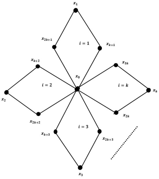
Figure 4. $F_{4,k}$ with labeling of vertices.

Theorem 3.

Let $k>2$ and $G\cong F_{5,k}$ be a friendship graph with blocks each of length 5 and $\left|V\left(F_{5,k}\right)\right|=4k+1$ then, $rn\left(F_{5,k}\right)\le 8k+1.$

Proof. 

Define the map $L$ as follows:

Let $k$ be an odd number, and then

$$L\left(x_{jk+i}\right)=\left\{\begin{array}{cc}0,& i=j=0\\ 3+i-1,& j=\mathrm{0,1}\le i\le k\\ k+2\left(i+1\right),& j=\mathrm{1,1}\le i\le k\\ 3k+2\left(i+1\right),& j=\mathrm{2,1}\le i\le k\\ 5k+3i+1,& j=\mathrm{3,1}\le i\le k\end{array}\right.$$

while

$$L\left(x_{jk+i}\right)=\left\{\begin{array}{cc}0,& i=j=0\\ 3+i-1,& j=0,1\le i\le k\\ k+2\left(i+1\right),& j=1,1\le i\le k\\ 3k+4,& j=2,i=1\\ 3k+3+2i& j=2,2\le i\le k\\ 5k+5& j=3,i=1\\ 5k+1+3i& j=3,2\le i\le k\end{array}\right.$$

whenever $k$ is an even number.

Since $diam\left(F_{5,k}\right)=4$, we claim to prove that $\left|L\left(x_u\right)-L\left(x_v\right)\right|\ge 5-d\left(x_u{,x}_v\right)$ for all $x_u,x_v\in V\left(F_{5,k}\right)$ and $u\ne v$.

Case 1. Let $j=0,1\le i\le k$, and then, $\left|L\left(x_0\right)-L\left(x_{jk+i}\right)\right|=\left|0-(3+i-1)\right|=2+i.$ Since $d\left(x_0{,x}_{jk+i}\right)=2.$ Then, $\left|L\left(x_0\right)-L\left(x_{jk+i}\right)\right|\ge 5-d\left(x_0{,x}_{jk+i}\right).$

Case 2. Let $j=1,1\le i\le k$, and then $\left|L\left(x_0\right)-L\left(x_{jk+i}\right)\right|=\left|0-(k+2i+2)\right|=k+2i+2\ge 3.$ Since $d\left(x_0{,x}_{jk+i}\right)\in \left\{\mathrm{1,2}\right\}.$ Consequently, $\left|L\left(x_0\right)-L\left(x_{jk+i}\right)\right|\ge 5-d\left(x_0{,x}_{jk+i}\right).$

Case 3. Let $j=2,1\le i\le k$ then, $\left|L\left(x_0\right)-L\left(x_{jk+i}\right)\right|=\left|0-(3k+2i+2)\right|=3k+2i+2\ge 3.$ Moreover, $d\left(x_0{,x}_{jk+i}\right)\in \left\{\mathrm{1,2}\right\}.$ Consequently, $\left|L\left(x_0\right)-L\left(x_{jk+i}\right)\right|\ge 5-d\left(x_0{,x}_{jk+i}\right)$.

Case 4. Let $j=3,1\le i\le k$, and then

$\left|L\left(x_0\right)-L\left(x_{jk+i}\right)\right|=\left|0-\left(5k+3i+1\right)\right|=5k+3i+1\ge 3.$ Since, $d\left(x_0{,x}_{jk+i}\right)\in \left\{\mathrm{1,2}\right\},$ then, $\left|L\left(x_0\right)-L\left(x_{jk+i}\right)\right|\ge 5-d\left(x_0{,x}_{jk+i}\right).$

Case 5. Let $j=0,1\le i<t\le k$, and then $\left|L\left(x_{jk+i}\right)-L\left(x_{jk+t}\right)\right|=\left|L\left(x_i\right)-L\left(x_t\right)\right|=t-i\ge 1.$

Since $d\left(x_{jk+i}{,x}_{jk+t}\right)=4$, then $\left|L\left(x_{jk+i}\right)-L\left(x_{jk+t}\right)\right|\ge 5-d\left(x_{jk+i}{,x}_{jk+t}\right).$

Similarly, we can prove that the radio condition holds for every pair of vertices from $V\left(F_{5,k}\right)$, and $L$ is a radio labeling of $F_{5,k}$ that proved $rn\left(F_{5,k}\right)\le 8k+1.$ □

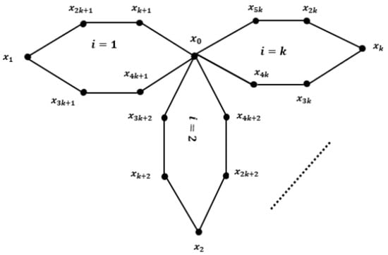
For more illustrations, $F_{5,k}$ with labeling of vertices is presented in Figure 5.

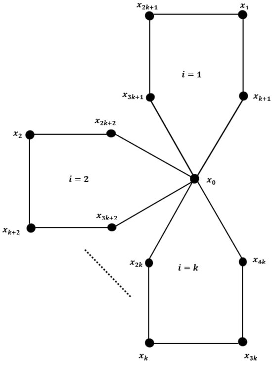
Figure 5. $F_{5,k}$ with labeling of vertices.

Theorem 4.

Let $k>2,F_{6,k}$ be a friendship graph with blocks each of length 6 and $\left|V\left(F_{6,k}\right)\right|=5k+1$ and then $rn\left(F_{6,k}\right)\le 17k+1.$

Proof. 

Define the map $L$ as follows:

$$L\left(x_{jk+i}\right)=\left\{\begin{array}{cc}0,& i=j=0\\ 4+i-1,& j=\mathrm{0,1}\le i\le k\\ k+6,& j=1,i=1\\ k+10+3\left(i-2\right)& j=\mathrm{1,2}\le i\le k\\ 4k+4+3i& j=\mathrm{2,1}\le i\le k\\ 7k+7& j=3,i=1\\ 7k+11+5\left(i-2\right)& j=\mathrm{3,2}\le i\le k\\ 12k+5i+1& j=\mathrm{3,2}\le i\le k\end{array}\right.$$

Since $diam\left(F_{6,k}\right)=6$. From the above definition of the labeling function $L$ and Figure 6, one can prove that the radio condition $\left|L\left(x_u\right)-L\left(x_v\right)\right|\ge 7-d\left(x_u{,x}_v\right)$ holds for all $x_u,x_v\in V\left(F_{6,k}\right)$and $u\ne v$. Moreover, $rn\left(F_{6,k}\right)\le 17k+1$. □

Figure 6. $F_{6,k}$ with labeling of vertices.

A friendship $F_{6,k}$ with labeling of its vertices is shown in Figure 6.

3. Integer Linear Programming Model

A new mathematical formulation for the radio labeling problem is proposed for $F_{3,k},F_{4,k},F_{5,k},$ and $F_{6,k}$. We next describe the problem of finding the radio labeling problem for a graph in terms of an integer programming problem [4]. Let $G$ be a connected graph of order $n$ with $V\left(G\right)=\left\{u_1,u_2,\cdots ,u_n\right\}$ and let $D=\left[d_{ij}\right]$ be the distance matrix of $G$, that is, $d_{ij}=d\left(u_i,u_j\right)$ for $1\le i,j\le n.$ We suppose that $v_i$ are the labels of the vertices $u_i$ such that $1\le i\le n$. Now, we can introduce the mathematical model for the radio labeling problem as an integer programming model. We define the function $F$ by

$$\mathit{min}F=v_1+v_2+\cdots +v_n$$

subject to

$$\left|v_i-v_j\right|\ge diam+1-d\left(u_i,u_j\right)\mathrm{for}1\le i\le n-1;2\le j\le n\mathrm{and}i<j$$

where $v_1,v_2,\cdots ,v_n\in \left\{\mathrm{0,1}\right\}$

The radio number of the graph $G={max}_{1\le i\le n}\left\{v_i\right\}.$

4. Computational Study

We carried out a computational study to measure the efficiency of the proposed upper bounds by Theorems 1–4 compared to the results of the algorithms introduced in [3,4]. Moreover, the comparison between the results of those Theorems and the mathematical model introduced in Section 3 is also presented. All of these are compatible with a PC with a Core i7 CPU@2.8 GHz, 8 GB of RAM, and a 64-bit operating system. The computational studies were carried out using MATLAB R2016a and the MS Windows 7 Professional system.

According to the upper bound of the radio number of $F_{3,k}$, Table 1 and Figure 7 show that the proposed results in Theorem 1 outperform the proposed results in [3] for $k$ when it is odd. When k is even, the same results occur. On the other hand, the proposed results in Theorem 1 outperform the proposed results in [4] for every k.

Table 1. A comparison among our results, [3], and integer programming results [4] for $F_{3,k}$.

$\mathit{k}$	$\mathit{n}$	Saha [3]		ILPM [4]		Theorem 1
		$\mathit{r}\mathit{n}\left({\mathit{F}}_{3,\mathit{k}}\right)$	CPU Time	$\mathit{r}\mathit{n}\left({\mathit{F}}_{3,\mathit{k}}\right)$	CPU Time	$\mathit{r}\mathit{n}\left({\mathit{F}}_{3,\mathit{k}}\right)$
1	3	4	0.024824	4	0.07009	3
2	5	5	0.026428	7	0.056758	5
3	7	8	0.028891	10	0.060813	7
4	9	9	0.035933	13	0.066483	9
5	11	12	0.035994	16	0.067994	11
6	13	13	0.03913	19	0.07225	13
7	15	16	0.03958	22	0.073795	15
8	17	17	0.041326	25	0.078172	17
9	19	20	0.044408	28	0.078172	19
10	21	21	0.045015	31	0.080299	21
11	23	24	0.047039	34	0.088287	23
12	25	25	0.047221	37	0.102373	25
13	27	28	0.048065	40	0.160287	27
14	29	29	0.04859	43	0.182859	29
15	31	32	0.092601	46	0.272814	31

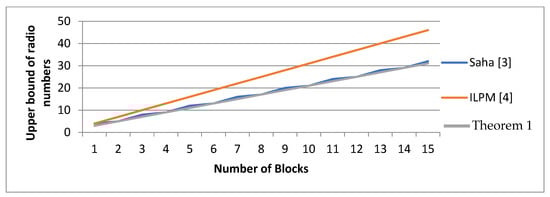
Figure 7. A comparison among our results, the Saha algorithm, Saha, L., et al., 2012 [3]; and integer programming according to the upper bound of the radio number of $F_{3,k}$ from Badr, et al., 2020 [4].

According to the running time, Table 1 and Figure 8 show that the proposed results in Theorem 1 take the constant time complexity O(1), while the proposed results in [3] take O(n³). On the other hand, the proposed results in Theorem 1 take less time than the proposed results in [4].

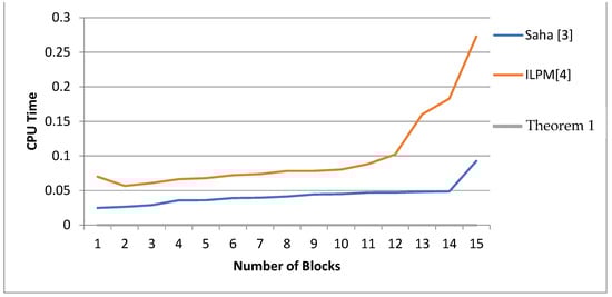
Figure 8. A CPU time comparison among our results, the Saha algorithm, Saha, L., et al., 2012 [3]; and integer programming of $F_{3,k}$ from Badr, et al., 2020 [4].

According to the upper bound of the radio number of $F_{4,k}$, Table 2 and Figure 9 show that the proposed results in Theorem 2 outperform the proposed results in [3] for $k=1,2$.

Table 2. A comparison among our results, [3], and integer programming results [4] for $F_{4,k}$.

$\mathit{k}$	$\mathit{n}$	Saha [3]		ILPM [4]		Theorem 2
		$\mathit{r}\mathit{n}\left({\mathit{F}}_{4,\mathit{k}}\right)$	CPU Time	$\mathit{r}\mathit{n}\left({\mathit{F}}_{4,\mathit{k}}\right)$	CPU Time	$\mathit{r}\mathit{n}\left({\mathit{F}}_{4,\mathit{k}}\right)$
1	4	10	0.025561	11	0.051869	8
2	7	16	0.027393	17	0.053149	15
3	10	22	0.02758	23	0.055986	22
4	13	29	0.028133	30	0.056235	29
5	16	36	0.030245	37	0.067974	36
6	19	43	0.030387	44	0.067994	43
7	22	50	0.031081	51	0.06921	50
8	25	57	0.031635	58	0.071135	57
9	28	64	0.031749	65	0.07225	64
10	31	71	0.035689	72	0.073031	71
11	34	78	0.038289	79	0.106774	78
12	37	85	0.043385	86	0.107721	85
13	40	92	0.043505	93	0.160287	92
14	43	99	0.044422	100	0.182859	99
15	46	106	0.054716	107	0.200691	106

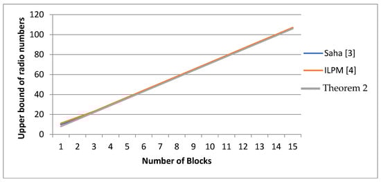
Figure 9. A comparison among our results, the Saha algorithm, Saha, L., et al., 2012 [3]; and integer programming according to the upper bound of the radio number of $F_{4,k}$ from Badr, et al., 2020 [4].

For $k=3,4,\dots ,15$, the same results occur. On the other hand, the proposed results in Theorem 2 outperform the proposed results in [4] for every k.

According to the running time, Table 2 and Figure 10 show that the proposed results in Theorem 2 take the constant time complexity O(1) while the proposed results in [3] take O(n³). On the other hand, the proposed results in Theorem 2 take less time than the proposed results in [4]

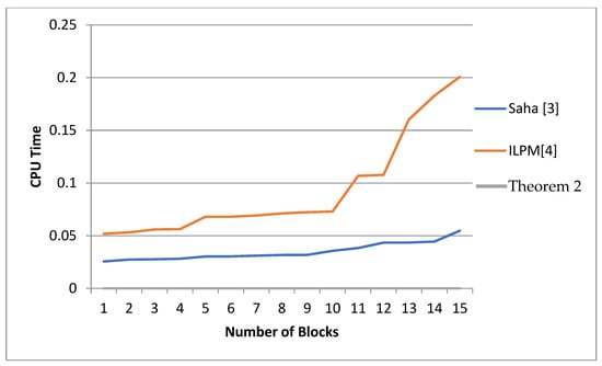
Figure 10. A CPU time comparison among our results, the Saha algorithm, Saha, L., et al., 2012 [3]; and integer programming of $F_{4,k}$ from Badr, et al., 2020 [4].

According to the upper bound of the radio number of $F_{5,k}$, Table 3 and Figure 11 show that the proposed results in Theorem 3 outperform the proposed results in [3] for $k=1$.

Table 3. A comparison among our results, [3], and integer programming results [4] for $F_{5,k}$.

$\mathit{k}$	n	Saha [3]		ILPM [4]		Theorem 3
		$\mathit{r}\mathit{n}\left({\mathit{F}}_{5,\mathit{k}}\right)$	CPU Time	$\mathit{r}\mathit{n}\left({\mathit{F}}_{5,\mathit{k}}\right)$	CPU Time	$\mathit{r}\mathit{n}\left({\mathit{F}}_{5,\mathit{k}}\right)$
1	5	12	0.013394	14	0.033658	9
2	9	17	0.013676	24	0.038117	17
3	13	25	0.021828	35	0.048892	25
4	17	33	0.045767	46	0.050592	33
5	21	41	0.159417	57	0.053916	41
6	25	49	0.170631	68	0.057428	49
7	29	57	0.212698	79	0.064091	57
8	33	65	0.248107	90	0.124051	65
9	37	73	0.253468	101	0.133257	73
10	41	81	0.285491	112	0.162882	81
11	45	89	0.286759	123	0.221091	89
12	49	97	0.450209	134	0.23193	97
13	53	105	0.454764	145	0.23485	105
14	57	113	0.604194	156	0.312935	113
15	61	121	0.621928	167	0.317238	121

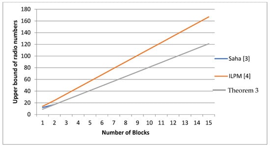
Figure 11. A comparison among our results, the Saha algorithm, Saha, L., et al., 2012 [3]; and integer programming according to the upper bound of the radio number of $F_{5,k}$ from Badr, et al., 2020 [4].

For $k=2,\mathrm{3,4},\cdots ,15$, the same results occur. On the other hand, the proposed results in Theorem 3 outperform the proposed results in [4] for every $k$.

According to the running time, Table 3 and Figure 12 show that the proposed results in Theorem 3 take the constant time complexity O(1), while the proposed results in [3] take O(n³). On the other hand, the proposed results in Theorem 3 take less time than the proposed results in [4].

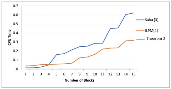
Figure 12. A CPU time comparison among our results, the Saha algorithm, Saha, L., et al., 2012 [3]; and integer programing of $F_{5,k}$ from Badr, et al., 2020 [4].

According to the upper bound of the radio number of $F_{6,k}$, Table 4 and Figure 13 show that the proposed results in Theorem 4 outperform the proposed results in [3] for $k=1$. For $k=2,\mathrm{3,4},\cdots ,15$, the same results occur. On the other hand, the proposed results in Theorem 4 outperform the proposed results in [4] for every k.

Table 4. A comparison among our results, [3], and integer programming results [4] for $F_{6,k}$.

$\mathit{k}$	n	Saha [3]		ILPM [4]		Theorem 4
		$\mathit{r}\mathit{n}\left({\mathit{F}}_{6,\mathit{k}}\right)$	CPU Time	$\mathit{r}\mathit{n}\left({\mathit{F}}_{6,\mathit{k}}\right)$	CPU Time	$\mathit{r}\mathit{n}\left({\mathit{F}}_{6,\mathit{k}}\right)$
1	6	22	0.026524	24	0.033143	18
2	11	36	0.029344	44	0.038123	35
3	16	52	0.030768	62	0.040921	52
4	21	69	0.049229	80	0.042084	69
5	26	86	0.092921	98	0.045056	86
6	31	103	0.094403	117	0.046653	103
7	36	120	0.129486	136	0.046656	120
8	41	137	0.258403	155	0.047893	137
9	46	154	0.281746	174	0.04914	154
10	51	171	0.314351	193	0.05036	171
11	56	188	0.417131	212	0.060892	188
12	61	205	0.488938	231	0.06789	205
13	66	222	0.59044	250	0.075292	222
14	71	239	0.703049	269	0.08014	239
15	76	256	1.08618	288	0.09014	256

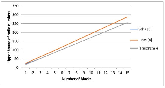
Figure 13. A comparison among our results, the Saha algorithm, Saha, L., et al., 2012 [3]; and integer programming according to the upper bound of the radio number of $F_{6,k}$ from Badr, et al., 2020 [4].

According to the running time, Table 4 and Figure 14 show that the proposed results in Theorem 4 take the constant time complexity O(1), while the proposed results in [3] take O(n³). On the other hand, the proposed results in Theorem 4 take less time than the proposed results in [4].

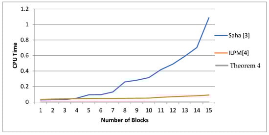
Figure 14. A CPU time comparison among our results, the Saha algorithm, Saha, L., et al., 2012 [3]; and integer programming of $F_{6,k}$ from Badr, et al., 2020 [4].

5. Conclusions

In this paper, the radio labeling of friendship networks ($F_{3,k},F_{4,k},F_{5,k}$, and $F_{6,k}$) are studied. Additionally, a mathematical model is proposed to find the upper bound of ($F_{3,k},F_{4,k},F_{5,k},$ and $F_{6,k}$). A computational study is presented to prove the efficiency of our results compared to the previous results. Finally, the empirical study shows that the proposed results overcome the previous results according to the upper bound of the radio number and the running time. In future work, we will find an upper bound of the radio number of general friendship networks $F_{n,k}$. Moreover, new algorithms and development of known algorithms will be proposed to find the radio numbers of the different radio networks.

References

- Hale, W.K. Frequency assignment: Theory; Applications. Proc. IEEE 1980, 68, 1497–1514. [Google Scholar] [CrossRef]
- Chartrand, G.; Erwin, D.; Harary, F.; Zhang, P. Radio labelings of graphs. Bull. Inst. Combin. Appl. 2001, 33, 77–85. [Google Scholar]
- Saha, L.; Panigrahi, P. A graph Radio k-coloring algorithm. Lect. Notes Comput. Sci. 2012, 7643, 125–129. [Google Scholar]
- Badr, E.M.; Moussa, M.I. An upper bound of radio k-coloring problem and its integer linear programming model. Wirel. Netw. 2020, 26, 4955–4964. [Google Scholar] [CrossRef]
- Li, X.; Mak, V.; Zhou, S. Optimal radio labelings of complete m-array trees. Discret. Appl. Math. 2010, 158, 507–515. [Google Scholar] [CrossRef]
- Liu, D.D.-F. Radio number for trees. Discret. Math. 2008, 308, 1153–1164. [Google Scholar]
- Liu, D.D.-F.; Xie, M. Radio number for square of cycles. Congr. Numer. 2004, 169, 105–125. [Google Scholar]
- Liu, D.D.-F.; Xie, M. Radio number for square paths. Ars Comb. 2009, 90, 307–319. [Google Scholar]
- Liu, D.D.-F.; Zhu, X. Multi-level distance labelings for paths and cycles. SIAM J. Discret. Math. 2005, 19, 610–621. [Google Scholar] [CrossRef]
- Morris-Rivera, M.; Tomova, M.; Wyels, C.; Yeager, Y. The radio number of Cn × Cn. Ars Comb. 2012, 103, 81–96. [Google Scholar]
- Ortiz, P.; Martinez, P.; Tomova, M.; Wyels, C. Radio numbers of some generalized rism graphs. Discuss. Math. Graph Theory 2011, 311, 45–62. [Google Scholar]
- Reddy, V.S.; Iyer, V.K. Upper bounds on the radio number of some trees. Int. J. Pure Appl. Math. 2011, 71, 207–215. [Google Scholar]
- Saha, L.; Panigrahi, P. On the Radio number of Toroidal grids. Aust. J. Comb. 2013, 55, 273–288. [Google Scholar]
- Saha, L.; Panigrahi, P. A lower bound for radio k-chromatic number. Discret. Appl. Math. 2015, 192, 87–100. [Google Scholar] [CrossRef]
- Zhang, P. Radio labellings of cycles. Ars Comb. 2002, 65, 21–32. [Google Scholar]
- ELrokh, A.; Badr, E.; Al-Shamiri, M.M.A.; Ramadhan, S. Upper bounds of radio number for triangular snake and double triangular snake Graphs. J. Math. 2022, 2022, 3635499. [Google Scholar] [CrossRef]
- Badr, E.; Almotairi, S.; Elrokh, A.; Abdel-Hady, A.; Almutairi, B. An Integer Linear Programming Model for Solving Radio Mean Labeling Problem. IEEE Access 2020, 8, 162343–162349. [Google Scholar] [CrossRef]
- Badr, E.; Nada, S.; Al-Shamiri, M.M.A.; Abdel-Hay, A.; ELrokh, A. A novel mathematical model for radio mean square labeling problem. J. Math. 2022, 2022, 3303433. [Google Scholar] [CrossRef]
- Badr, E.M.; Elgendy, H. A hybrid water cycle—Particle swarm optimization for solving the fuzzy underground water confined steady flow. Indones J. Electr. Eng. Comput. Sci. 2020, 19, 492–504. [Google Scholar] [CrossRef]
- Badr, E.M.; Almotiari, S. On a dual direct cosine simplex type algorithm and its computational behavior. Math. Probl. Eng. 2020, 2020, 7361092. [Google Scholar] [CrossRef]
- Bloom, G.S.; Golomb, S.W. Applications of Numbered Undirected Graphs. Proc. Ofthe Inst. Electr. Electron. Eng. 1977, 65, 562–570. [Google Scholar] [CrossRef]
- Bosck, J. Cyclic Decompositions, Vertex Labellings and Graceful Graphs; Decompositions of Graphs; Kluwer Academic Publishers: Dordrecht, The Netherlands, 1990; pp. 57–76. [Google Scholar]
- Frucht, R. Graceful Numbering of Wheels and Other Related Graphs. Ann. N. Y. Acad. Sci. 1979, 319, 219–229. [Google Scholar] [CrossRef]
- Frucht, R.; Gallian, J.A. Labeling Prisms. Ars Comb. 1988, 26, 69–82. [Google Scholar]
- Gallian, J.A. A Dynamic Survey of Graph Labeling. Electron. J. Comb. 2021, 24. [Google Scholar] [CrossRef]
- Graham, R.L.; Sloane, N.J.A. On Additive Bases and Harmonious Graphs. SIAM J. Algebr. Discret. Methods 1980, 1, 382–404. [Google Scholar] [CrossRef]
- Golomb, S.W. How to Number a Graph, Graph Theory and Computing; Read, R.C., Ed.; Academic Press: Cambridge, MA, USA, 1972; pp. 23–37. [Google Scholar]
- Rosa, A. On Certain Valuations of the Vertices of a Graph, Theory of Graphs; International Symposium, Rome, Italy, 1966; Gordon and Breach: Philadelphia, PA, USA, 1967; pp. 349–355. [Google Scholar]
- Singh, G.S. A Note on Graceful Prisms. Natl. Acad. Sci. Lett. 1992, 15, 193–194. [Google Scholar]
- Acharya, B.D.; Gill, M.K. On the Index of Gracefulness of a Graph and the Gracefulness ofTwo-Dimensional Square Lattice Graphs. Indian J. Math. 1981, 23, 81–94. [Google Scholar]
Disclaimer/Publisher’s Note: The statements, opinions and data contained in all publications are solely those of the individual author(s) and contributor(s) and not of MDPI and/or the editor(s). MDPI and/or the editor(s) disclaim responsibility for any injury to people or property resulting from any ideas, methods, instructions or products referred to in the content. |
© 2023 by the authors. Licensee MDPI, Basel, Switzerland. This article is an open access article distributed under the terms and conditions of the Creative Commons Attribution (CC BY) license (https://creativecommons.org/licenses/by/4.0/).