The Application of the Random Time Transformation Method to Estimate Richards Model for Tree Growth Prediction

Abstract

To model dynamic systems in various situations results in an ordinary differential equation of the form ${\displaystyle \frac{dy}{dt}}=g(y,t,\theta )$, where g denotes a function and $\theta$ stands for a parameter or vector of unknown parameters that require estimation from observations. In order to consider environmental fluctuations and numerous uncontrollable factors, such as those found in forestry, a stochastic noise process ${ϵ}_t$ may be added to the aforementioned equation. Thus, a stochastic differential equation is obtained: ${\displaystyle \frac{d{Y}_t}{dt}}=f(Y_t,t,\theta )+{ϵ}_t$. This paper introduces a method and procedure for parameter estimation in a stochastic differential equation utilising the Richards model, facilitating growth prediction in a forest’s tree population. The fundamental concept of the approach involves assuming that a deterministic differential equation controls the development of a forest stand, and that randomness comes into play at the moment of observation. The technique is utilised in conjunction with the logistic model to examine the progression of an agricultural epidemic induced by a virus. As an alternative estimation method, we present the Random Time Transformation (RTT) method. Thus, this paper’s primary contribution is the application of the RTT method to estimate the Richards model, which has not been conducted previously. The literature often uses the logistic or Gompertz models due to difficulties in estimating the parameter form of the Richards model. Lastly, we assess the effectiveness of the RTT Method applied to the Chapman–Richards model using both simulated and real-life data.

1. Introduction

Least-squares or likelihood methods typically treat differential equations with error-prone measurements based on diffusion-type stochastic modifications of the differential equation. We study the performance of likelihood methods based on the substitution of a Random Time Transformation (RTT) as an argument in the solution of the original deterministic differential equation. This method can be used to simultaneously estimate parameters describing multiple differential equations based on data with dependent measurement errors. We use this technique to estimate parameters in a stochastic differential equation based on the Richards model. In this paper, we propose the use of the RTT technique applied for the first time to the Chapman–Richards model for tree growth. Therefore, the aim of this paper is to present some model-fitting methods based on stochastic differential equations. The discussion is mainly inspired by the works of Delattre et al. [1], García [2,3], Gushchin and Kuchler [4], Lacus [5], Kloeden and Platen [6,7] and Seber et al. [8], among others. Let us consider some growth models used for different applications, such as Gompertz, Von Bertalanffy, Chapman–Richards, Weibull, Chanter or Fletcher. An ordinary differential equation characterises their deterministic form to model the growth rate $\frac{dy}{dt}=g(y,t,\theta )$ or the relative growth rate $\frac{1}{y}\frac{dy}{dt}=g(y,t,\theta )$, where $\theta$ is an unknown parameter that should be estimated from empirical observations, equidistant or not, of one or more individuals of the species. In addition, a process of stochastic noise $ϵ=\left({ϵ}_t\right)$ must be included to account for fluctuations in the mean set and many other uncontrollable factors. Thus, in its more general form, the process Y describing growth satisfies the following Stochastic Differential Equation (SDE) model (1):

$$\frac{d{Y}_t}{dt}=f(Y_t,t,\theta ,{ϵ}_t)$$

(1)

Generally, the process represented by $ϵ$ is additive white noise giving origin to the equation

$$d{Y}_t=a(Y_t,t,\theta )dt+b(Y_t,t,\theta )d{W}_t$$

(2)

where a and b are functions and $d{W}_t$ is the one dimensional standard Wiener process. It is also possible to replace the white noise $d{W}_t$ for a colored noise $d{V}_t$ that satisfies an SDE in turn $d{V}_t=(a{V}_t+d\left(t\right))dt+d{W}_t$. For more details on non-white noise disturbances, see Kashyap and Ramachandra Rao [9]. It is important to note that the model (2) would, in principle, lead to the absurd situation where $Y_t$ decreases or becomes negative with time; this is a price that must be paid for the mathematical treatment of the problem; see García [2].

We observe that in Liang et al. [10], the research delves into a complex topic in stochastic processes and statistical physics, exploring the intricate behaviour of fractional Brownian motion when subjected to non-linear clocks. It examines how these non-linearities affect various aspects of the motion, including diffusion, statistical properties and the concept of aging. Understanding these phenomena is crucial for gaining insight into complex systems where standard Gaussian assumptions and linear time scales may not hold, such as in the study of turbulent flows, financial markets or biological processes. This approach allows researchers to explore the intricate interplay between time transformations, statistical properties and the dynamics of complex stochastic processes, shedding light on the non-standard behaviour observed in systems with anomalous diffusion and non-Gaussian statistics. Now, how does this work relate to random time transformation? RTT is a broader concept that encompasses any transformation of time intervals or time scales in a stochastic process. It can include various methods of changing the time variable to produce different statistical behaviour. The introduction of non-linear clocks is effectively a form of RTT because it transforms the standard time scale of fBm into a non-linear and potentially random one.

For our problem in the field of forestry, we know that efficient forest management is a very complex issue. A natural forest is made up of trees of different ages, lands of diverse qualities, and, in native forests, differing species. Good planning for forest management requires reliable projections of growth and yield. In many situations, it is sufficient to adjust a simple growth curve, to describe the course of stand variables over time. With more intensive management, however, these variables are manipulated by silvicultural interventions that can vary in date and intensity, and it becomes necessary to predict the behaviour of stands in a variety of different circumstances.

The applications of stochastic differential equations (SDEs) in forest management offer a wealth of valuable insights and problem-solving potential in a variety of scenarios. While we have briefly touched on these applications earlier, let us now explore concrete, real-world situations where these approaches can be used effectively, as SDEs are proving invaluable in modelling the dynamics of forest growth, incorporating variables such as climate, soil quality and tree species. By solving these equations, forest managers can determine the ideal time to harvest trees, maximizing yield while maintaining sustainability principles. SDEs are also well suited to capturing the inherent uncertainty in forest growth factors, including disease outbreaks, insect infestations and climate variability. Using these models, forest managers can assess the risk associated with these events and implement targeted mitigation strategies. In addition, forests act as important carbon sinks, and SDEs facilitate the estimation of a forest’s carbon storage capacity over time. This supports carbon credit calculations and ensures compliance with environmental regulations. By incorporating ecological dynamics, SDEs enable forest managers to assess the impact of different management approaches on biodiversity. This informs decisions that balance timber production with conservation objectives. Within the forestry sector, SDEs are also useful for optimizing the entire supply chain, from harvesting to transport to processing plants. Given the uncertainty of factors such as transportation costs and demand, forest companies can streamline operations and reduce costs. Finally, forests provide a range of ecosystem services, including water purification, recreation and wildlife habitat. SDEs facilitate the quantification of the economic value associated with these services, thereby facilitating decision making and policy formulation.

The paper, besides Section 1, contains seven sections and is organised as follows. In Section 2 and Section 3, we provide the necessary theoretical background and concisely describe the growth curve model used here. In Section 4, we present the estimation of the Richards model using the Random Time Transformation. Section 5 is concerned with the likelihood function of the variables ${\tilde{Y}}_{t_j}^i,1\le i\le ,1\le j\le n.$ The results are presented in Section 6. Finally, some conclusions are given in Section 7.

2. Data and Fit of the Model

Different ways of observing Y give different ways of estimating $\theta$. In this paper, fitting the model (2) means estimating the parameter $\theta$ from observations of the process Y. Growth data are usually cross-sectional or longitudinal. In a cross-sectional study, data are collected from a population at one point in time. In a longitudinal study, data are collected from the same sample over time. Often the information collected has both characteristics. For example, each tree in a stand that is measured several times will produce data that we call mixed. It is useful to distinguish between the growth model of an individual and the probabilistic model of the data applied to it. Indeed, if we postulate the existence of a growth model based on the SDE, the likelihood of the observed data (probabilistic model of the observations) will take different forms depending on the observation strategy of the process, whether it is continuous or discrete in time, or longitudinal or cross-sectional. We then study the critical class of linear models and some special cases of growth models. We then present a model and an estimation procedure for predicting the growth of a group of trees. Our growth model is based on a deterministic differential equation where randomness is introduced during the observation. To illustrate this technique, we use an application to the Chapman–Richards growth model.

3. Richards Model

The model

$${\displaystyle \frac{dy}{dt}}=\eta y^{\delta }-\gamma y$$

(3)

The von Bertalanffy growth model was proposed in 1938 [11] as a mechanistic model of animal growth. The model is based on the difference between the metabolic forces of anabolism and catabolism (Bertalanffy [12]). Richards (1959) [13] doubted the theoretical validity and usefulness of the von Bertalanffy models as a description of the growth mechanism. However, he noted that Equation (3) with $\delta$ treated as a free parameter provided a flexible family of curves with an arbitrarily placed inflection point. In other words, the von Bertalanffy growth model is a mathematical model that can be used to describe the growth of animals. The model is based on the assumption that the rate of growth is proportional to the difference between the animal’s current weight and its maximum weight, and the model is flexible enough to fit a wide range of growth curves, and it is still widely used today in biology and other fields. It is easy to observe that the growth rate is positive, but the final size constraint, $\delta$ and $\gamma$, in Equation (3), must be negative if $\delta >1$. By imposing the condition ${\displaystyle \frac{dy}{dt}}=0$ at $y=\alpha$, we can write the Equation (3) as

$${\displaystyle \frac{dy}{dt}}=\kappa y\left[{\displaystyle \frac{{(y/\alpha )}^{\delta -1}-1}{1-\delta }}\right];\delta \ne 1$$

(4)

where $\kappa =\eta (1-\delta ){\alpha }^{(\delta -1)}$ is the rate of growth, $\delta$ is the inflection point, and $\alpha$ is the asymptotic height reached by the tree. See Seber et al. [8] for more details. This Richards model includes the monomolecular model ($\delta =0$), von Bertalanffy model ($\delta =\frac{2}{3}$), logistic model ($\delta =2$) and (by taking the limit as $\delta \to 1$) Gompertz equation. A comprehensive Richards function is often used in the quantitative analysis of plant growth; see, for example, [13,14,15,16,17,18]. The Richards function is very flexible and has a horizontal asymptote, and its graph has a characteristic sigmoid shape. The Richards model can be transformed into a linear form. However, the linear form of the Richards function cannot be used to determine its constant parameters using analytical methods because the growth model under consideration has up to three independent coefficients. The constant coefficients of the Richards function can be calculated (after estimating their values) using numerical methods. The solution of (4) is

$$y_t=\alpha {\left[1+({\left(\frac{y_0}{\alpha }\right)}^{1-\delta }-1)e^{-\kappa (t-t_0)}\right]}^{\frac{1}{1-\delta }};y_0=y_{t_0}$$

(5)

where we need $\kappa ,\delta$ positive and $(1-\delta )e^{-\kappa t_0}.\le 1$; see Seber et al. [8] for more details.

The following Figure 1 and Figure 2 show two Richards model simulations and the exact solution based on an Euler scheme for different values of the parameters; the thick line is the exact solution. Certainly, it is possible to use other scheme methods such as Milstein or other alternatives. The stochastic version of the Richards model is given by:

$$d{Y}_t=\kappa Y_t\left(\frac{{\left(\frac{Y_t}{\alpha }\right)}^{\delta -1}-1}{1-\delta }\right)dt+d{W}_t$$

(6)

For the simulation, we use the Euler scheme

$$Y_i=Y_{i-1}+\kappa Y_{i-1}\left(\frac{{\left(\frac{Y_{i-1}}{\alpha }\right)}^{\delta -1}-1}{1-\delta }\right)h+{\Delta W}_{i}i=2,\dots ,n+1Y_1=Y_0$$

(7)

where the increments $\Delta W_i$ are identically and independently distributed random variables $\mathcal{N}(0,h)$ in each subinterval $t_i\le t\le t_{i+1}.$

The two-parameter models have a growth rate per capita that is symmetric near the inflection point at the midpoint of the carrying capacity. However, this is not the case for n populations of large mammals; see Fowler [19]. A three-parameter model, such as the Richards model, may fit better to an asymmetric growth rate per capita because of the additional form parameter (see Sibly et al. [20]) and the focus on stochastic differential equations to model growth as presented as an alternative to the classical models. The study by Ghosh et al. [21] examines the Richards four-parameter non-linear growth model, which is a very versatile framework for characterizing various growth phenomena. Typically, this model is formulated as a non-linear differential equation. However, a transformation exists which converts it into a solvable linear differential equation. Alternatively, a more comprehensive approach involving stochastic differential equations (SDEs) can be adopted. These SDEs are generally derived by introducing a stochastic component into the differential equation of the deterministic model. Consequently, this stochastic component is often assumed to follow a Gaussian white noise stochastic process. In addition, the approximating SDE can simplify the model by eliminating one parameter, reducing the four-parameter stochastic differential equation Richards model to a linear SDE model that can be solved using Ito calculus. In particular, fitting the Richards model to data has historically encountered challenges related to poor conditioning and convergence. These problems often arise when there is insufficient observable curve data to provide a reliable initial estimate of the final magnitude parameter, $\alpha$. Overcoming these challenges typically involves numerical methods to solve the non-linear least squares problem, as described in Dennis et al. [22]. However, it remains a complex endeavor to establish the existence of a least squares estimate for non-linear least square problems. Theorems on the existence of such estimates for certain functions can be found in [23,24]. For these reasons, we study an alternative method for estimating the parameters of the Richards model.

4. Estimation of the Richards Model

White et al. [25], consider the estimates in the Richards model to be based on a discrete approach to the error term. The estimate is calculated using the method of non-linear squares. On the other hand, García [2] considers it convenient to use ordinary ordinary differential equations as the basis for modelling the growth of trees, specifically equations of the form

$${\displaystyle \frac{dY}{dt}}=g\left(Y\right)$$

(8)

where Y is the height and t is the time. In his paper, García affirms that growth is affected by fluctuations in the environment and adds a term for random error to the term of random error into the equation, leading to a stochastic differential equation. He then integrates the SDE, the solution of which is discretizing the solution to estimate the parameters using maximum likelihood. In this case, the estimation of the parameters of interest seems to be insensitive to changes in the variance. He also points out that the properties of these estimates are uncertain and possibly inconsistent. As an estimation alternative, we propose a method of Random Time Transformation (RTT), credited to Bassan et al. [26], which was used with the logistic model to study the evolution of an agricultural plague. The model is applied to fit disease progression curves using actual data obtained from disease assessments of melon plants afflicted with the Zucchini Yellow Mosaic Virus (ZYMV). The parameter estimation approach used in this study corresponds to an inference problem in a stochastic process, where the dynamics of the growth of a tree or group of trees is modelled by an Ordinary Differential Equation, (ODE), where randomness is introduced at the time of observation of the process. This is equivalent to a calibration problem. In fact, most linear regression problems involving prediction or estimation require the determination of the Y corresponding to a given X. The calibration problem (or inverse estimation or discrimination) is the inverse of the above, where we have a given value of Y and want to determine X. Random time transformations find extensive application in Ergodic Theory and Topological Dynamics, which are often linked to skew product transformations, as exemplified in Adler et al. [27]. More specifically, the concept of Random Time Transformation (RTT) is rooted in ergodic theory, a branch of mathematics and statistical physics concerned with the long-term behaviour of dynamical systems. The ergodic theory focuses on understanding how systems evolve and how they approach equilibrium or invariant distributions. Asymmetric transformations are an essential part of this theory, as they represent transformations that do not preserve symmetry or invariance, making them particularly relevant for understanding real-world processes where randomness and asymmetry play a significant role. RTT emerges as a mathematical tool to bridge the gap between ergodic theory and asymmetric transformations. It addresses the idea that in many real-world scenarios, the underlying dynamics are not symmetric, and traditional methods of analysis may not apply. RTT introduces randomness into the time parameter of a dynamical system, reflecting the intrinsic stochasticity or uncertainty present in many natural processes. In this way, RTT allows us to study how a system’s behaviour evolves over random, asymmetric time intervals, capturing the complex dynamics that may be missed by traditional symmetric approaches. In essence, RTT extends the scope of ergodic theory to better model and analyse systems subject to asymmetry and randomness, providing valuable insights into a wide range of scientific and practical applications. The underlying concept of random time transformation becomes evident through practical instances. For instance, when assessing the age of a machine, it is more accurately represented by the number of hours it has operated rather than the time since its purchase. Similarly, the age of a car is better described by its mileage rather than the year it was manufactured. In cases where plant diseases are transmitted by insects, modelling the infection’s incidence at a time t within area A is more precise when considering the total number of insect hours rather than t alone. Moreover, if local environmental or climatic conditions lead to a temporary increase in the insect population, time effectively speeds up, as discussed in Bassan et al. [26]. An interesting application of the RTT method is due to the recent work of Alon et al. [28], on the SIR epidemiological equations, which model new infected and removed cases as roughly proportional to the current number of infected cases in an attempt to uncover the growth pattern of COVID-19. In our case, the essential idea of the method consists of supposing that a deterministic differential equation governs the growth of a tree and that randomness is introduced at the time of the observation. Moreover, the randomness enters at the time of observation. We use the Richards equation to present the method in our forestry context. We assume, therefore, that the growth of each tree is governed by the ordinary differential equation:

$$d{Y}_t^i=A_i\left(Y_t^i\right)dt,i=1,2,\cdots ,p$$

(9)

where p is the total numbers of trees and the function $A_i$ depends on some unknown parameter ${\theta }_i$, but $Y_t^i$ is not observable. However, what is observed is the process ${\tilde{Y}}_t^i=Y_{T_t}^i$, where $T_t$ is a process of time change, which does not necessarily increase. For example, $T_t$ may be a Brownian movement or Ornstein–Uhlenbeck process. In this paper, we will use the Brownian time change; we chose the Random Time method for its easiness to estimate the parameters in the Richards model, since if we work with the diffusion method that additively incorporates a process of error to estimate the parameters, serious numeric difficulties are presented to estimate the parameter $\delta$ (inflection point of the curve). Then, $\delta$ is close to one, as shown in Lipser and Shiryayev [29]. RTT is used for the first time to model the growth of trees based on the Richards model, which presents a major challenge in the estimation of its parameters as indicated in Ratkowski [30]. An alternative to estimating the Richards model appears in the work of Román–Román and Torres–Ruiz [31]. In their paper, a stochastic diffusion model related to a reformulation of the Richards growth curve is proposed and the problem of the maximum likelihood estimation for the parameters of the process is considered using metaheuristic optimisation algorithms such as simulated annealing and variable neighborhood search.

5. The Likelihood Function

Following the main ideas of Bassan et al. in [26], the likelihood function of the variables $({\tilde{Y}}_{t_j}^i,1\le i\le p,1\le j\le n)$ are represented using the elementary method of transforming variables, assuming increments of independent and identically distributed normal times with a covariance matrix of $\Sigma$ and real times. In $d_j=t_j-t_{j-1},$ we will use as basic random variables the Gaussian increments $z=(z_{i,j};1\le i\le p,1\le j\le n)$ where

$$z_{i,j}=d_j^{-\frac{1}{2}}(T_i\left(t_j\right)-T_i\left(t_{j-1}\right)-d_j);1\le i\le p,1\le j\le n$$

(10)

We will follow an approach that is technically similar to diffusion in the sense that it is based on modelling a likelihood for the increments of the observed process, and conceptually similar to the calibration approach in that the randomness is modelled as inherent in the time lag between the apparent time and chronological time.

The observed process is viewed as the solution to the deterministic differential equation but it is applied to a random time transformation of chronological time $t.$ The density of these basic random variables is evaluated at $z=(z_{i,j};1\le i\le p,1\le j\le n)$, where

$$z_{i,j}=d_j^{-\frac{1}{2}}(Y_i^{-1}\left(y_{ij}\right)-Y_i^{-1}\left(y_{i,j-1}\right)-d_j)=d_j^{-\frac{1}{2}}{\int }_{y_{i,j-1}}^{y_{ij}}\frac{dy}{A_i\left(y\right)}-d_j^{\frac{1}{2}}$$

(11)

corresponds to a Brownian time change, where $y_{ij}$ are the sizes of the trees at different times and $Y_i^{-1}\left(y_{ij}\right)$ is the observed time at time i. By the method of variable transformation, the density function of the random variables $({\tilde{Y}}_{t_j}^i,1\le i\le p,1\le j\le n),$ is expressible as the product of two terms, the density function of the basic random variables (10) and a Jacobian matrix. By defining $z_j={(z_{1,j},\cdots ,z_{p,j})}^{{}^{\prime }}$ and $\Sigma ={\sigma }^{2}I$ as the covariance matrix of $z_j$, the likelihood function can be expressed as

$$\mathcal{L}(y;\theta ,\Sigma )=f(z,\theta ,\Sigma )J(y;\theta ),$$

(12)

where J is the Jacobian matrix. In (9), the Jacobian as the determinant of the matrix

$${\displaystyle \frac{\partial z_{r,s}}{\partial y_{i,j}}}=\left\{\begin{array}{cc}\hfill {\displaystyle \frac{1}{\sqrt{d_j}{A}_i\left(y_{i,j}\right)}};\hfill & \hfill if(r,s)=(i,j)\hfill \\ \hfill -{\displaystyle \frac{1}{\sqrt{d_j}{A}_i\left(y_{i,j}\right)}};\hfill & \hfill if(r,s)=(i,j+1)\hfill \\ \hfill 0;\hfill & \hfill otherwise\hfill \end{array}\right.$$

is

$$J(y;\theta )={\left[\prod _{j=1}^n{d}_j\right]}^{-\frac{p}{2}}{\left[\prod _{i=1}^p\prod _{j=1}^n{A}_i\left(y_{ij}\right)\right]}^{-1}$$

(13)

and the density of the basic random variables (10) is given by

$$f(z,\theta ,\Sigma )={\left(2\pi \right)}^{-\frac{np}{2}}{\mid \Sigma \mid }^{-\frac{n}{2}}exp\{-\frac{1}{2}\sum _{j=1}^n{z}_j^{\prime }{\Sigma }^{-1}{z}_j\}$$

(14)

where the coordinates of $z_j$ are explicitly given by (11). In the case of the Richards model, $\theta =({\alpha }_1,\dots ,{\alpha }_p,\delta ,\kappa ,\sigma )$ is the vector of parameters, where ${\alpha }_i$ is the height of the tree, $\delta$ is the inflection point, $\kappa$ is the growth rate, $\sigma$ is the standard deviation and $Y=(y_{ij};1\le i\le p,1\le j\le n)$ are the sizes of the trees at different times. Presently, considering

$$d_j=1,j=1,\dots ,n,z_{ij}={\int }_{y_{i,j-1}}^{y_{ij}}\frac{dy}{A_i\left(y\right)}-1$$

(15)

with (by Equation (6))

$$A_i\left(y_{ij}\right)=\kappa y_{ij}\left[{\displaystyle \frac{{(y_{ij}/{\alpha }_i)}^{\delta -1}-1}{1-\delta }}\right],$$

(16)

we have that the likelihood function can be written as

$$\mathcal{L}(y,\theta ,{\sigma }^2)={\left(2\pi \right)}^{-np/2}{\sigma }^{-np}exp\left(-{\displaystyle \frac{1}{2{\sigma }^2}}\sum _{j=1}^n{z}_j^{\prime }{z}_j\right){\left[\prod _{i=1}^p\prod _{j=1}^n{A}_i\left(y_{ij}\right)\right]}^{-1}$$

(17)

The idea is to express the likelihood function in terms of a single parameter, optimizing it for each step and then estimating the parameters recursively. Other criteria are possible, such as least squares fitting, but we will not explore them in this paper.

We will now show the strategies for estimating the parameters $\sigma ,\kappa \mathrm{and}\delta$ in our model. The recursive procedure generates a surface by the optimal parameters of the likelihood function at each step, and the parameters are updated according to the following rules:

• $\sigma$ is updated by minimizing the mean squared error between the observed data and the predicted data;
• $\kappa$ is updated by maximizing the likelihood function;
• $\delta$ is updated by minimizing the Kullback–Leibler divergence between the prior and the posterior distribution.

Strategies to Estimate the Parameters

(a)

$\sigma$ Substitution

For the function $\mathcal{L}$ defined by (17), we find that the maximum of $\mathcal{L}(y;\theta ,{\sigma }^2)$, with respect to ${\sigma }^2$, is given by

$${\widehat{\sigma }}^2=\frac{1}{np}\sum _{i=1}^n\sum _{j=1}^{p}z{}_{ij}^2=\frac{1}{np}\sum _{j=1}^{n}z{}_j^{\prime }{z}_j$$

(18)

and replacing this value in $\mathcal{L}$, we have

$$\widehat{\mathcal{L}}(y;{\alpha }_1,\dots ,{\alpha }_p,\delta ,\kappa ,{\widehat{\sigma }}^2)={\left(2\pi e\right)}^{-\frac{np}{2}}{\widehat{\sigma }}^{-np}J(y;\theta )$$

(19)

On the other hand, given that

$$t=t_0+\frac{1}{\kappa }log\frac{[{\left(\frac{y_0}{{\alpha }_i}\right)}^{1-\delta }-1]}{[{\left(\frac{y}{{\alpha }_i}\right)}^{1-\delta }-1]}$$

(20)

and supposing increments of real-time $d_j=1,j=1,\cdots ,n$, we obtain that $z{}_{i,j}$ is given by

$$z{}_{i,j}=Y_i^{-1}\left(y_{ij}\right)-Y_i^{-1}\left(y_{i,j-1}\right)-1=\frac{1}{\kappa }log\frac{[{\left(\frac{y_{i,j-1}}{{\alpha }_i}\right)}^{1-\delta }-1]}{[{\left(\frac{y_{ij}}{{\alpha }_i}\right)}^{1-\delta }-1]}-1$$

(21)

Thus, replacing relation (21) in Equation (18), we obtain, finally,

$${\widehat{\sigma }}^2=\frac{1}{{\kappa }^{2}np}\sum _{i=1}^p\sum _{j=1}^n{\left[log\frac{[{\left(\frac{y_{i,j-1}}{{\alpha }_i}\right)}^{1-\delta }-1]}{[{\left(\frac{y_{ij}}{{\alpha }_i}\right)}^{1-\delta }-1]}-\kappa \right]}^2$$

(22)

We notice that the estimate of $\sigma$ will be available when $\kappa ,\delta ,{\alpha }_1,\dots ,{\alpha }_p$ have been estimated.

(b)

$\kappa$ Substitution

Let ${\widehat{\mathcal{L}}}_1(y;{\alpha }_1,\dots ,{\alpha }_p,\delta ,\kappa )=\widehat{\mathcal{L}}(y,{\alpha }_1,\dots ,{\alpha }_p,\delta ,\kappa ,\widehat{\sigma }),$ then we obtain

$${\widehat{\mathcal{L}}}_1=CD\left(y\right){\left[\frac{1}{np}\sum _{i=1}^p\sum _{j=1}^n{(log\frac{[{\left(\frac{y_{i,j-1}}{{\alpha }_i}\right)}^{1-\delta }-1]}{[{\left(\frac{y_{ij}}{{\alpha }_i}\right)}^{1-\delta }-1]}-\kappa )}^2\right]}^{-np}\prod _{i=1}^p\prod _{j=1}^n{\left[\frac{{\left(\frac{y_{ij}}{{\alpha }_i}\right)}^{\delta -1}-1}{1-\delta }\right]}^{-1}$$

(23)

where ${\displaystyle C={\left(2\pi e\right)}^{-\frac{np}{2}}\mathrm{and}D\left(y\right)=\left[\prod _{i=1}^p\prod _{j=1}^n{y}_{ij}\right]{}^{-1}.}$ Note that when maximizing ${\widehat{\mathcal{L}}}_1$ with respect to $\kappa$, it is equivalent to minimise the first term in brackets of Equation (23)

$$\frac{1}{np}\sum _{i=1}^p\sum _{j=1}^n{\left[log\frac{[{\left(\frac{y_{i,j-1}}{{\alpha }_i}\right)}^{1-\delta }-1]}{[{\left(\frac{y_{ij}}{{\alpha }_i}\right)}^{1-\delta }-1]}-\kappa \right]}^2$$

(24)

Thus, the optimum of (24) is reached in

$$\widehat{\kappa }=\frac{1}{np}\sum _{i=1}^p\sum _{j=1}^{n}log\frac{[{\left(\frac{y_{i,j-1}}{{\alpha }_i}\right)}^{1-\delta }-1]}{[{\left(\frac{y_{ij}}{{\alpha }_i}\right)}^{1-\delta }-1]}=\frac{1}{np}\sum _{i=1}^{p}log\frac{[{\left(\frac{y_{i0}}{{\alpha }_i}\right)}^{1-\delta }-1]}{[{\left(\frac{y_{in}}{{\alpha }_i}\right)}^{1-\delta }-1]}$$

(25)

We obtain, in this form, the estimate of $\widehat{\kappa }$, which is a function of ${\alpha }_1,\cdots ,{\alpha }_p$ and $1-\delta$.

(c)

${\alpha }_1,\cdots ,{\alpha }_p$ Substitution

Let us define ${\widehat{\mathcal{L}}}_2(y,{\alpha }_1,\cdots ,{\alpha }_p,\delta )={\widehat{\mathcal{L}}}_1(y,{\alpha }_1,\cdots ,{\alpha }_p,\delta ,\widehat{\kappa }).$ We want to find the maximum of ${\widehat{\mathcal{L}}}_2$ with respect to ${\alpha }_1,\cdots ,{\alpha }_p$. However, this is equivalent to minimizing the denominator of ${\widehat{\mathcal{L}}}_2.$ Thus, the following function is minimised

$${\widehat{\mathcal{L}}}_3={\left[\frac{1}{np}\sum _{i=1}^p\sum _{j=1}^n{\left\{(log\frac{[{\left(\frac{y_{i,j-1}}{{\alpha }_i}\right)}^{1-\delta }-1]}{[{\left(\frac{y_{ij}}{{\alpha }_i}\right)}^{1-\delta }-1]}-\widehat{\kappa }\right\}}^2\right]}^{np}\prod _{i=1}^p\prod _{j=1}^n\left[\frac{{\left(\frac{y_{ij}}{{\alpha }_i}\right)}^{\delta -1}-1}{1-\delta }\right]$$

(26)

Nevertheless, ${\widehat{\mathcal{L}}}_3$ reaches the global minimum when ${\displaystyle {\widehat{\alpha }}_i=\underset{j}{max}\left(y_{ij}\right),}$ that is,

$${\widehat{\mathcal{L}}}_3(y;{\widehat{\alpha }}_1,\dots ,{\widehat{\alpha }}_p,\delta )=0,\forall \delta .$$

(27)

Moreover, neither delta nor the other parameters can be estimated. However, the minimisation method available in MATLAB converge to a local minimum where the initial point is not close to $\widehat{{\alpha }_i},i=1,2,\cdots ,p.$ The problem is that ${\widehat{\mathcal{L}}}_2$ is unbounded as an ${\alpha }_1,\dots ,{\alpha }_p$ function and the maximum does not exist. In this case, we solve a constraint problem every time that ${\alpha }_i$ reaches the maximum of $y_{ij}.$ It is not difficult to show that the likelihood function ${\widehat{\mathcal{L}}}_2$ is unbounded for $\delta \ne 1.$

(d)

$\delta$ Estimate

We define ${\widehat{\mathcal{L}}}_4(y;\delta )={\widehat{\mathcal{L}}}_2({\widehat{\alpha }}_1,\dots ,{\widehat{\alpha }}_p,\delta ).$ Then, this function is maximised and $\widehat{\delta }$ is obtained. With this, $\widehat{\delta }$ is a numeric value, and ${\widehat{\mathcal{L}}}_4(y;\delta )$ is a function of y, from which we obtain ${\widehat{\alpha }}_1\left(\widehat{\delta }\right),\dots ,{\widehat{\alpha }}_p\left(\widehat{\delta }\right).$ Moreover, in this stage, we recover $\widehat{\kappa }$ as $\widehat{\kappa }=({\widehat{\alpha }}_1\left(\widehat{\delta }\right),\dots ,{\widehat{\alpha }}_p\left(\widehat{\delta }\right),\widehat{\delta })$ and later $\widehat{\sigma }$ as $\widehat{\sigma }=\widehat{\sigma }({\widehat{\alpha }}_1\left(\widehat{\delta }\right),\dots ,{\widehat{\alpha }}_p\left(\widehat{\delta }\right),\widehat{\kappa },\widehat{\delta }).$

Remark 1.

We note that there is another alternative for estimating the parameters in the SDE, which is to use the Radon–Nikodym theorem to find the likelihood function, maximise it to find the maximum likelihood estimators, and finally approximate the integral using numerical methods and Itô’s calculus.

6. Results

We will examine the performance of the (RTT) method applied to the Richards model, which we will analyse with simulated data, as one of the concerns of researchers is whether a particular model fits the data well. Nine cases were studied with known parameters to observe the behaviour of the bias in the parameters. For us, bias will be the difference between the exact values of the parameters and the values returned by the method, in this case by the simulations and not in the classic sense of the definition of bias. The instability in the estimation process can also result from the correlation between some parameters, as shown in the figures below. The instability of the variance can be due to the data and, in this case, very little can be conducted to improve these instabilities. We have to keep in mind that data are derived from living organisms which are typically correlated. Next, some simulated cases are presented. For each case, twenty runs were made considering eight trees and eight observations for each tree with the following graph being obtained. Now, we show the simulations for each one of the parameters of our model.

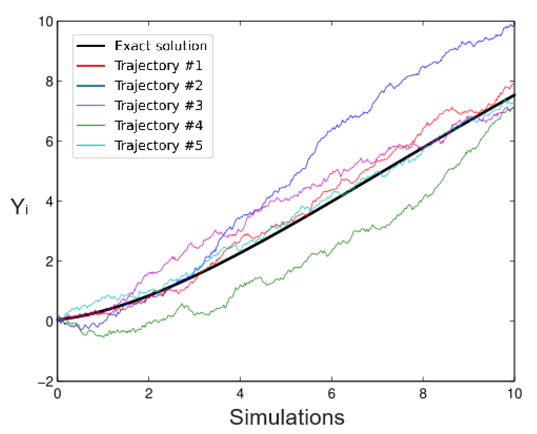
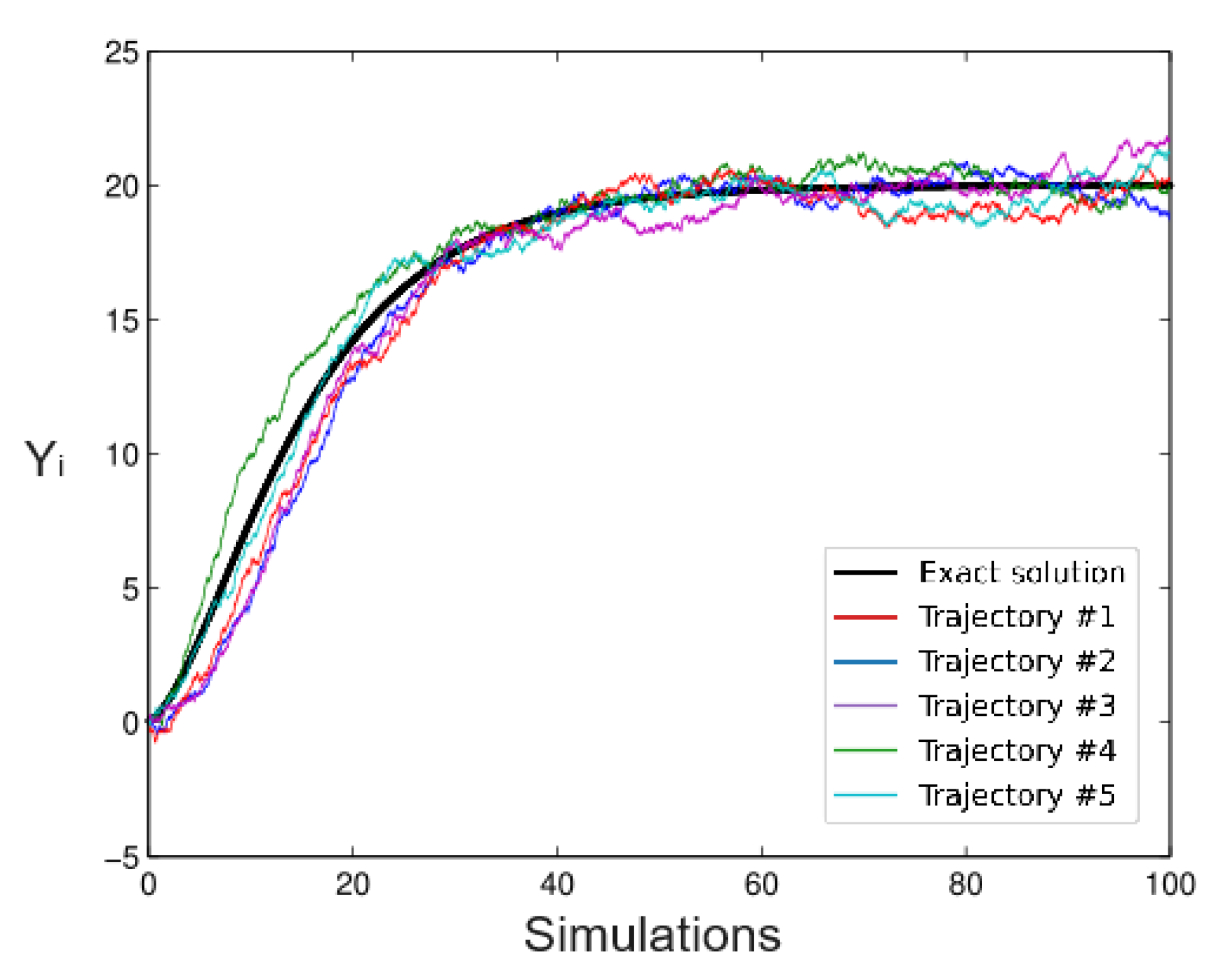
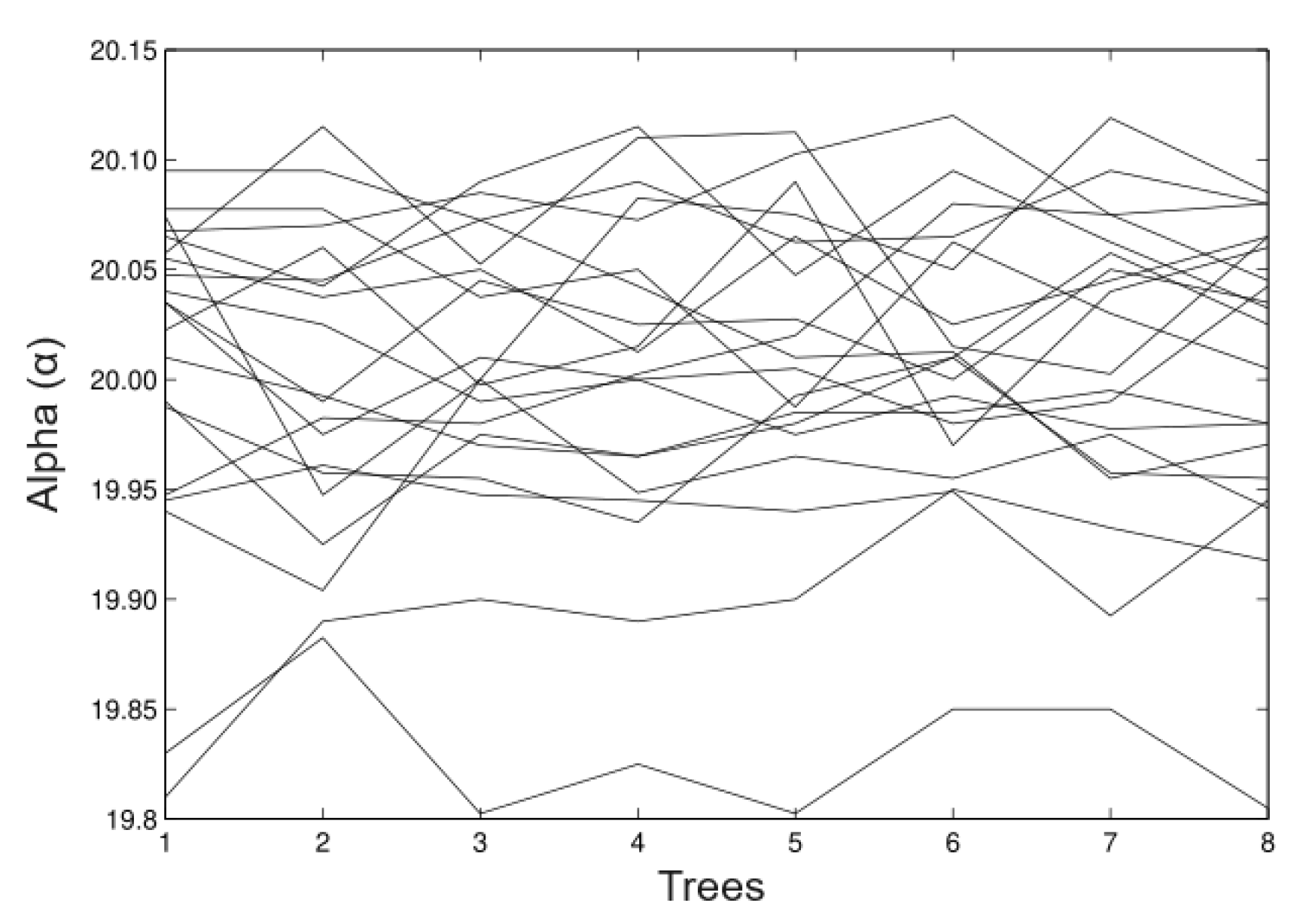
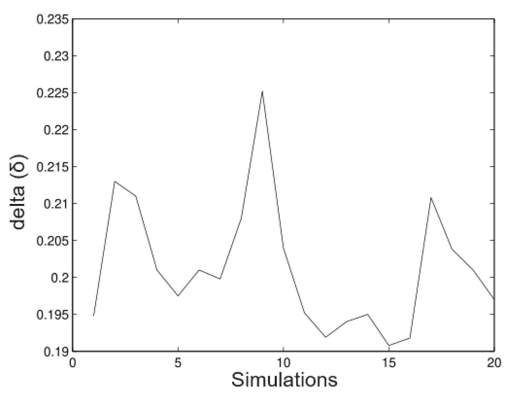
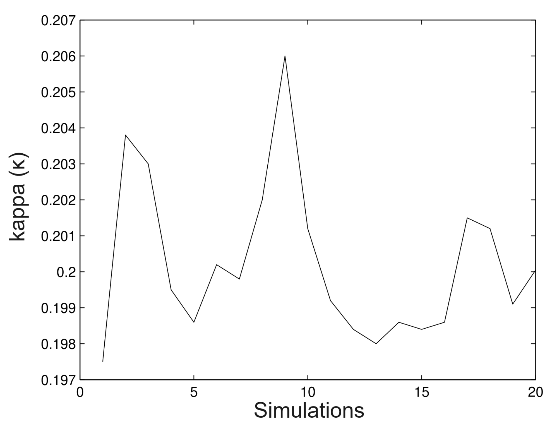
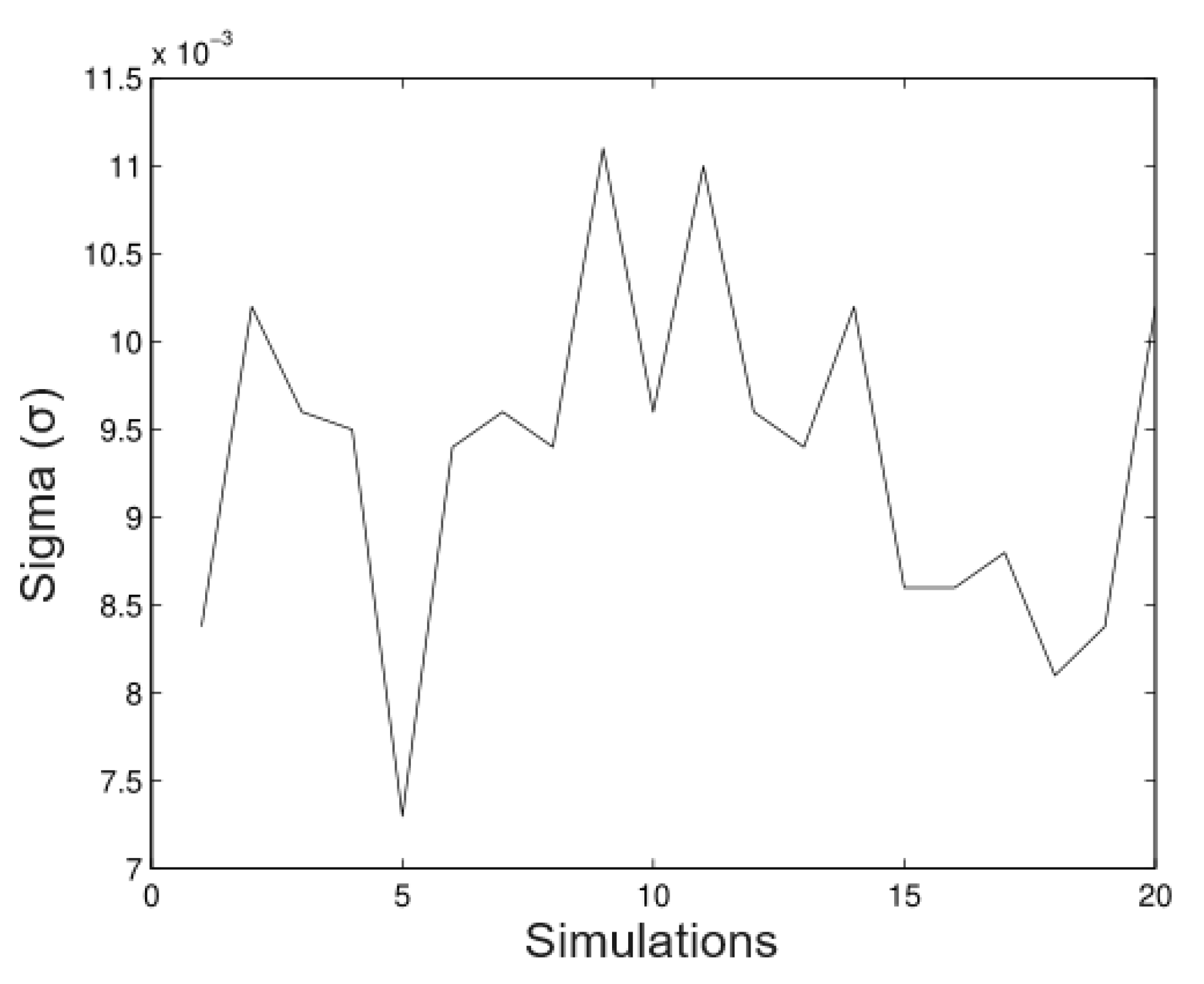
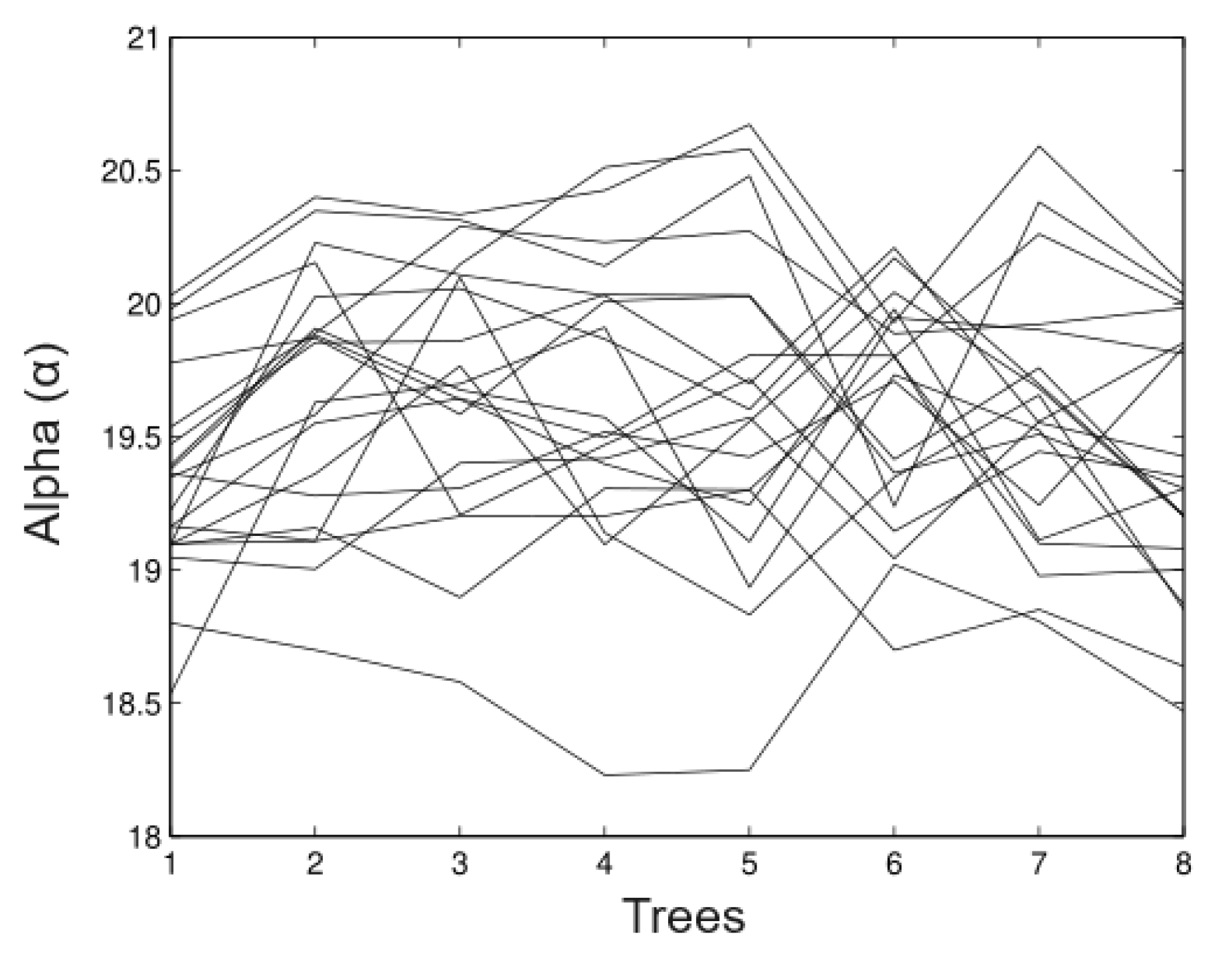
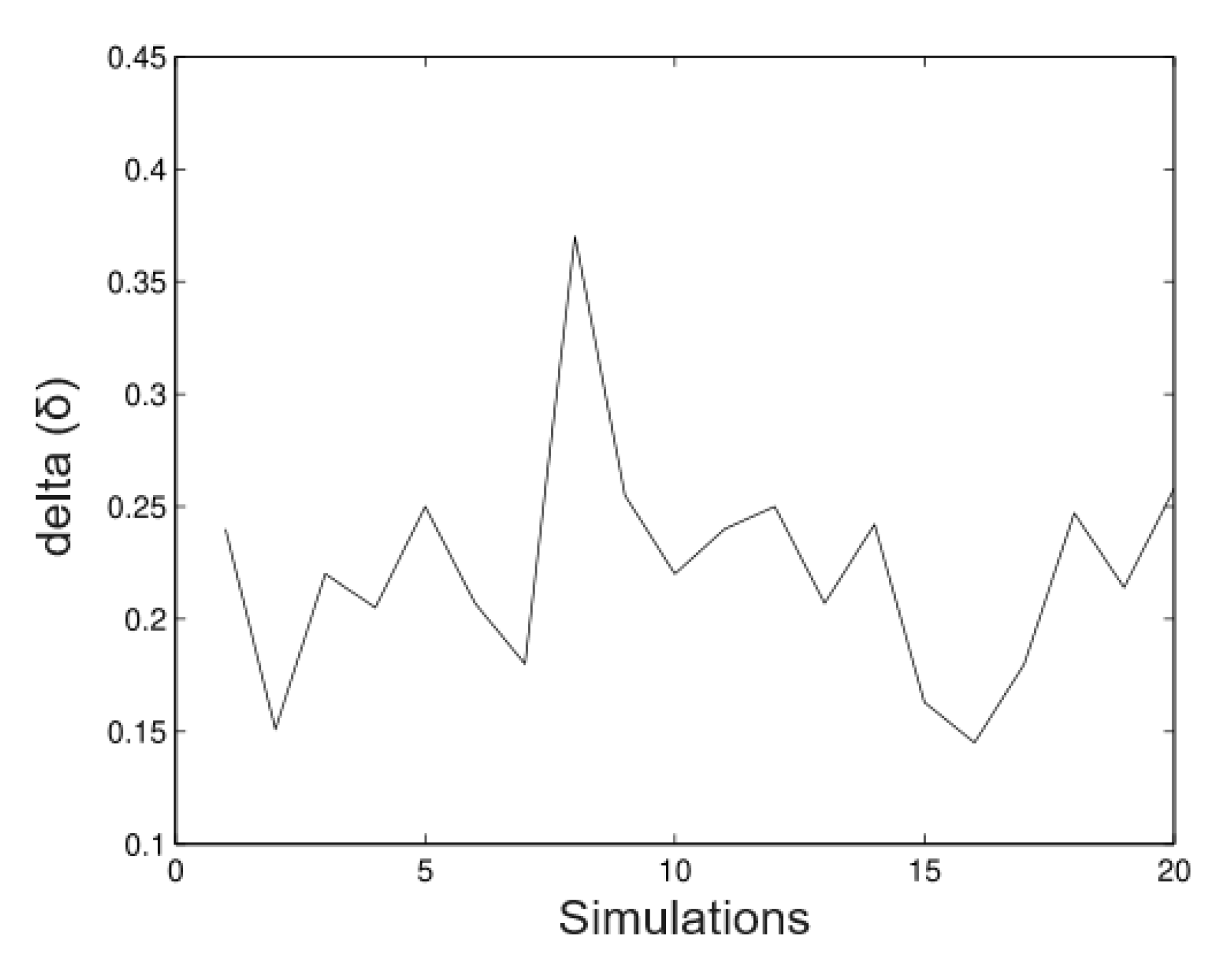
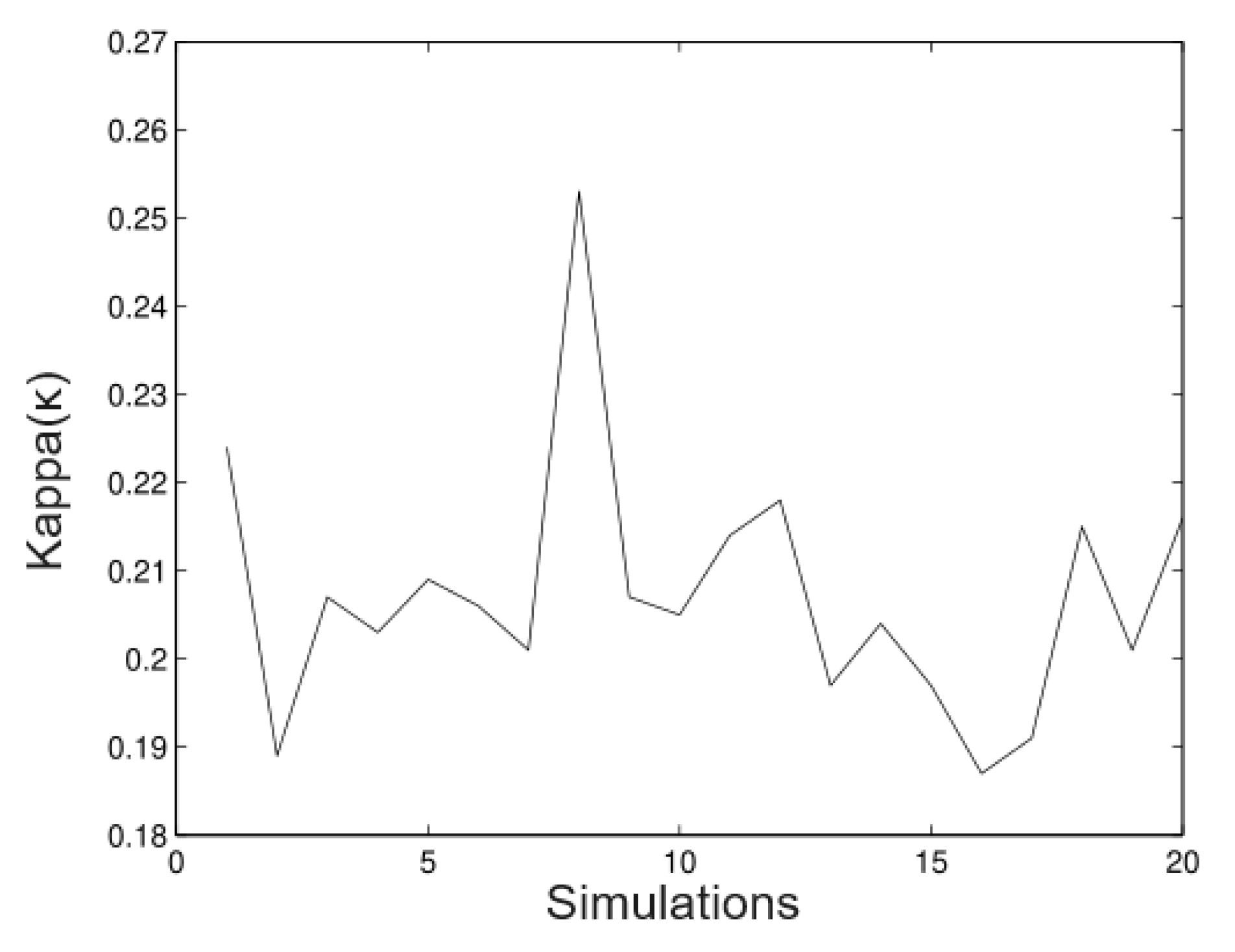
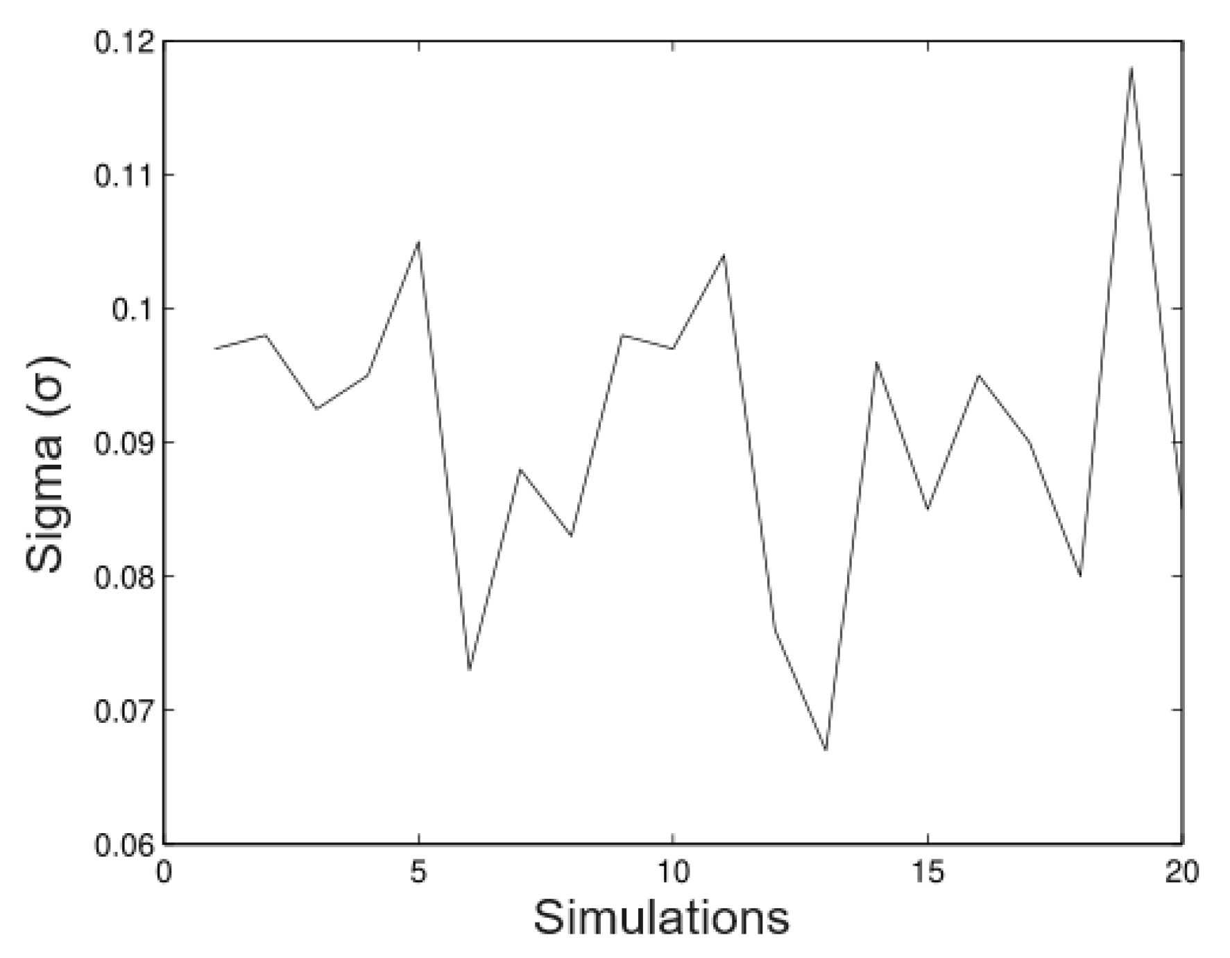
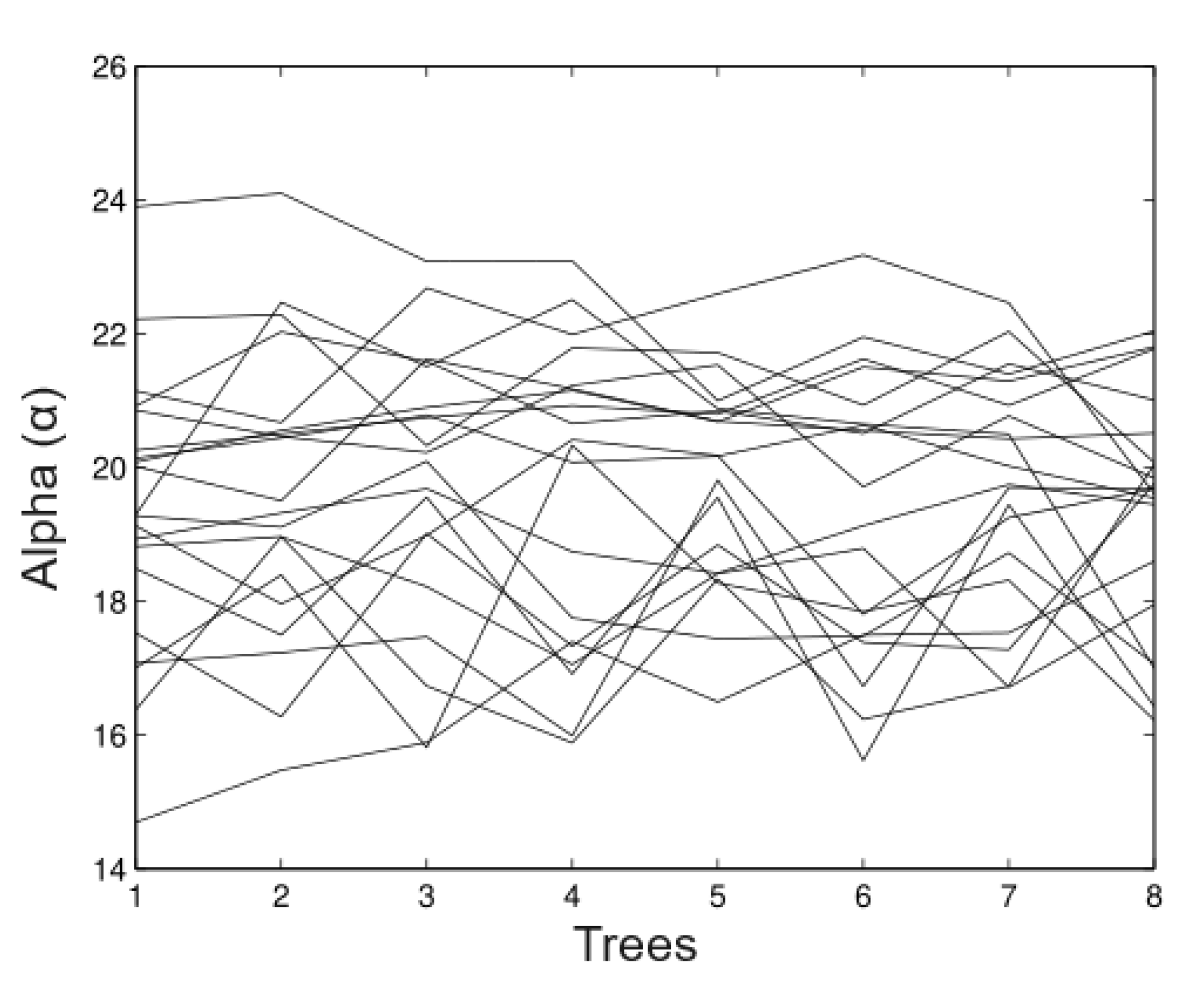
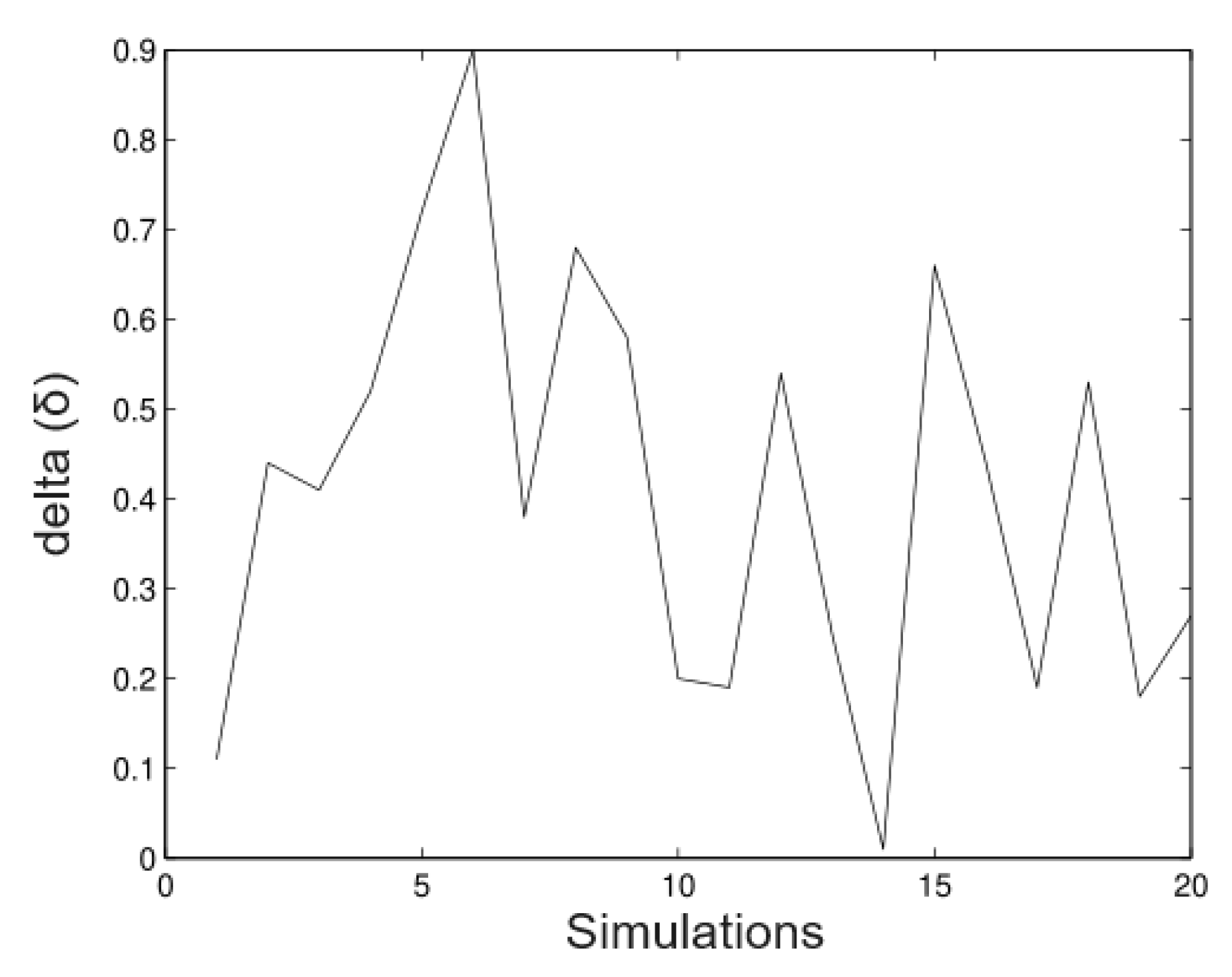
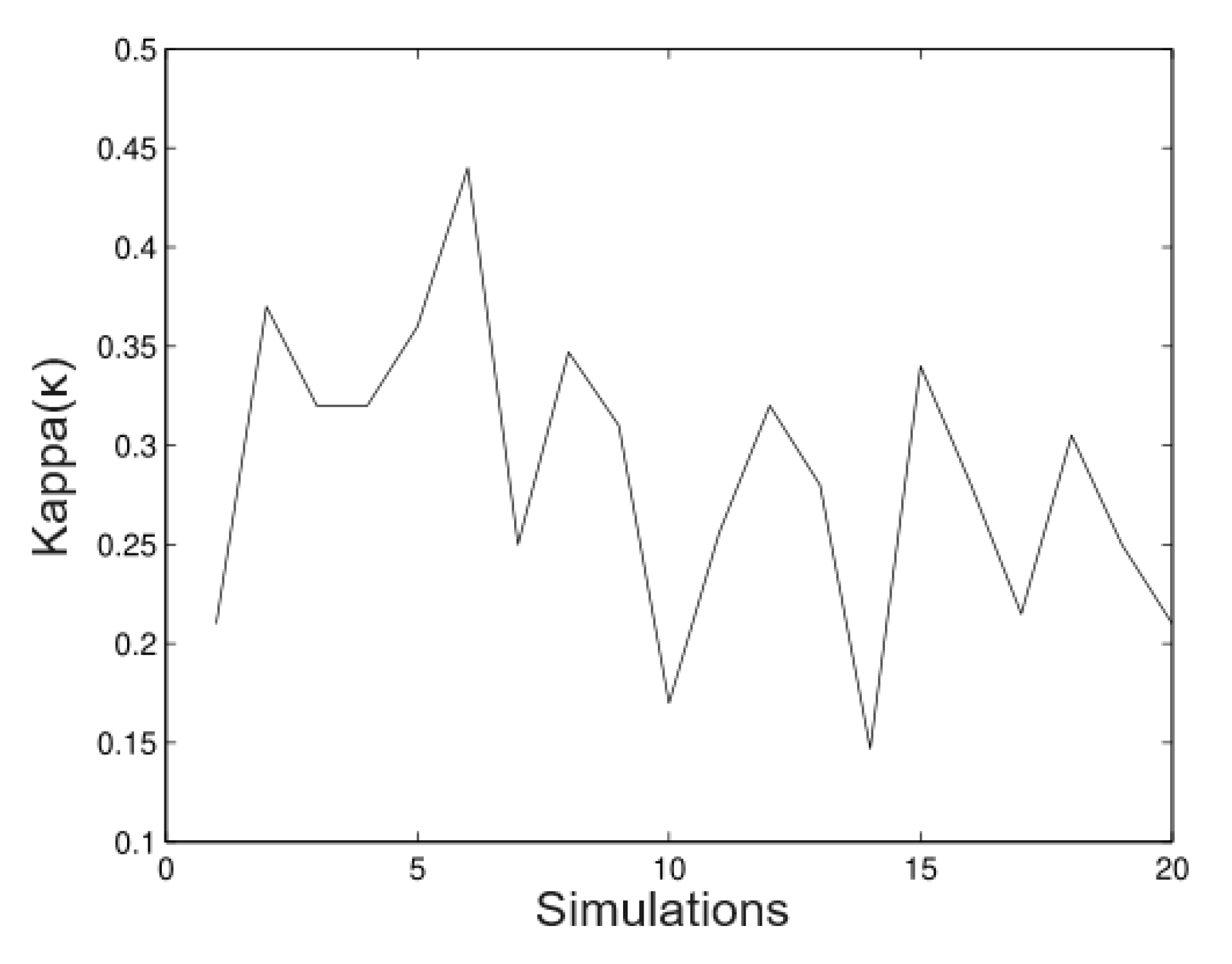
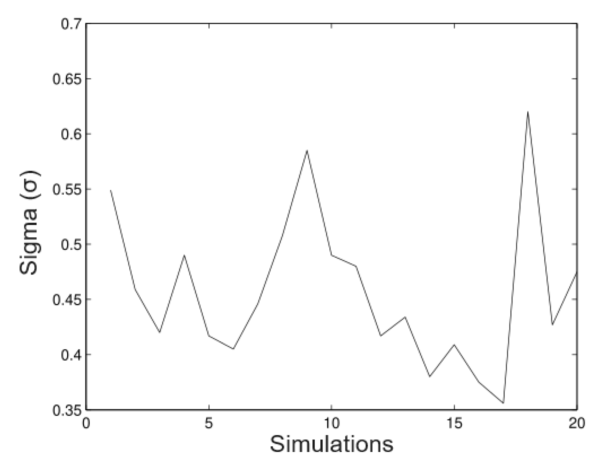
6.1. Simulated Data

Here, we provide a brief description of our simulations. Nine cases were analysed with known parameters to study how the method behaves, and to measure whether there is bias or not. Beginning with the simulation, we have to enter the number of data per tree (p) and the total number of trees (q). Then, a matrix M normally distributed $\mathcal{N}(0,1)$ i.i.d. of $p\times q$, where each column corresponds to one tree, has to be generated. The Random Time is generated by the matrix $NRT=T_i\times ones(p,q)$, with the order of $p\times q$, where $T_i$ is a square matrix with the order p with ones below the diagonal and zeros above the diagonal, and $ones(p,q)$ correspond to a matrix with order $p\times q$. Finally, there is the generation of the matrix X of $(p+1)\times q$, using the explicit solution of the Chapman–Richards model and Random Time. The matrix X contains the simulated to given values of $\delta ,\alpha ,\kappa$, and $\sigma$. For each case, runs considering $q=8$ trees and $p=8$ observations for each tree have been conducted, obtaining the following behaviour.

• Simulation 1: $\alpha$ = 20 (all trees), $\kappa$ = 0.2, $\delta$ = 0.2, and $\sigma$ = 0.01

In Figure 3, we observed that in the estimates of $\alpha ,$ the random time estimates the alpha values (maximum heights) relatively well. The fluctuations goes from 19.8 m to 20.12 m and the bias is the minimum in most of the cases. Figure 4 shows the appropriate behaviour of the $\delta$ parameter, although evidence exists in some cases that the method overestimates and underestimates the $\delta$ parameter simultaneously.

In Figure 5, we observe that the method is a good approximation to estimate the parameter $\kappa .$ With regard to the bias not being important in most of the cases, in Figure 6, we observe clearly that the method underestimates the $\sigma$ value, however, the bias is not important. In most of the simulated cases, the method has the same behaviour for the parameter. The next figures show a new simulation with the same parameters; however, in this case, we consider $\sigma =0.1.$

2.

Simulation 2: Alfa = 20 (all trees), $\kappa =0.2,\delta =0.2,\sigma =0.1$

In Figure 7, we observed that in the estimates of $\alpha ,$ the random time method estimates the alpha values (maximum heights) relatively well. The fluctuations go from 18.4 m to 20.52 m and the bias is the minimum in most of the cases. Figure 8 shows us the appropriate behaviour of the $\delta$ parameter, although evidence exists some cases that the method overestimates and underestimates the $\delta$ parameter simultaneously.

In Figure 9, we observe that the method is a good approximation to estimate the parameter $\kappa .$ With regard to the bias, it not important in most of the cases. In Figure 10, we observe clearly that the method underestimates the $\sigma$ value; however, the bias is not important. In most of the simulated cases, the method has the same behaviour for the parameter.

3.

Simulation 3: Alfa = 20 (all trees), $\kappa =0.2,\delta =0.2,\sigma =0.5$

The next figures show a new simulation with the same parameters; however, in this case, we consider $\sigma =0.5.$ We observe in Figure 11, Figure 12, Figure 13 and Figure 14 that in these cases the method does not estimate the parameters well; it underestimates the $\sigma$ value (as well as $\alpha$ values), but, on the other hand, it overestimates the $\kappa$ value (as well as the $\delta$ value). This shows that this technique is very sensitive to big values on the variance. This has effects on the trajectories of the solution of the stochastic differential equation. By increasing the variance, the trajectories will move away from the mean of the process. If the variance is small, the trajectories will evolve around the mean. A way to control the variability and ensure bounded growth is to fix a bound for the variance from a sampling of the process.

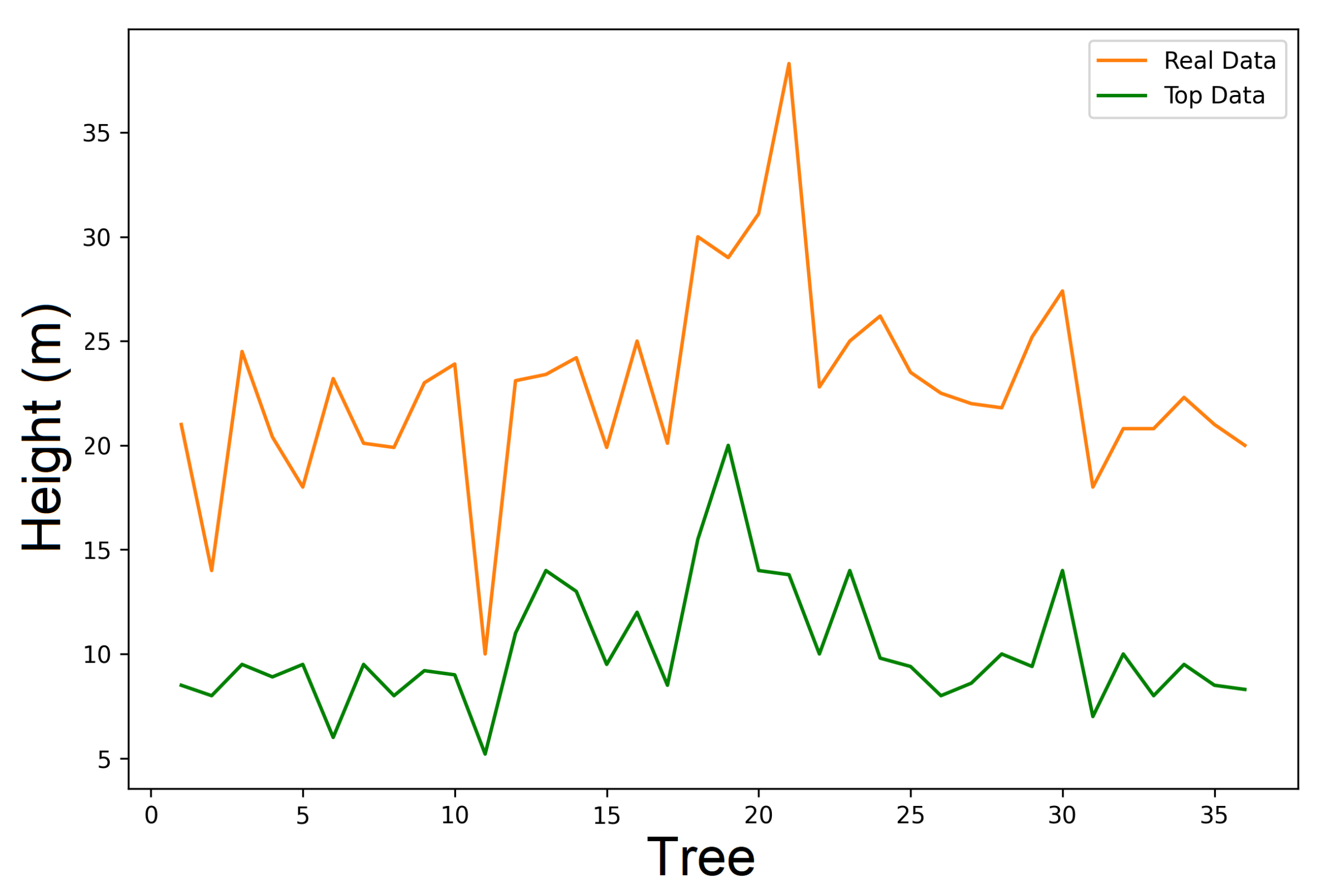
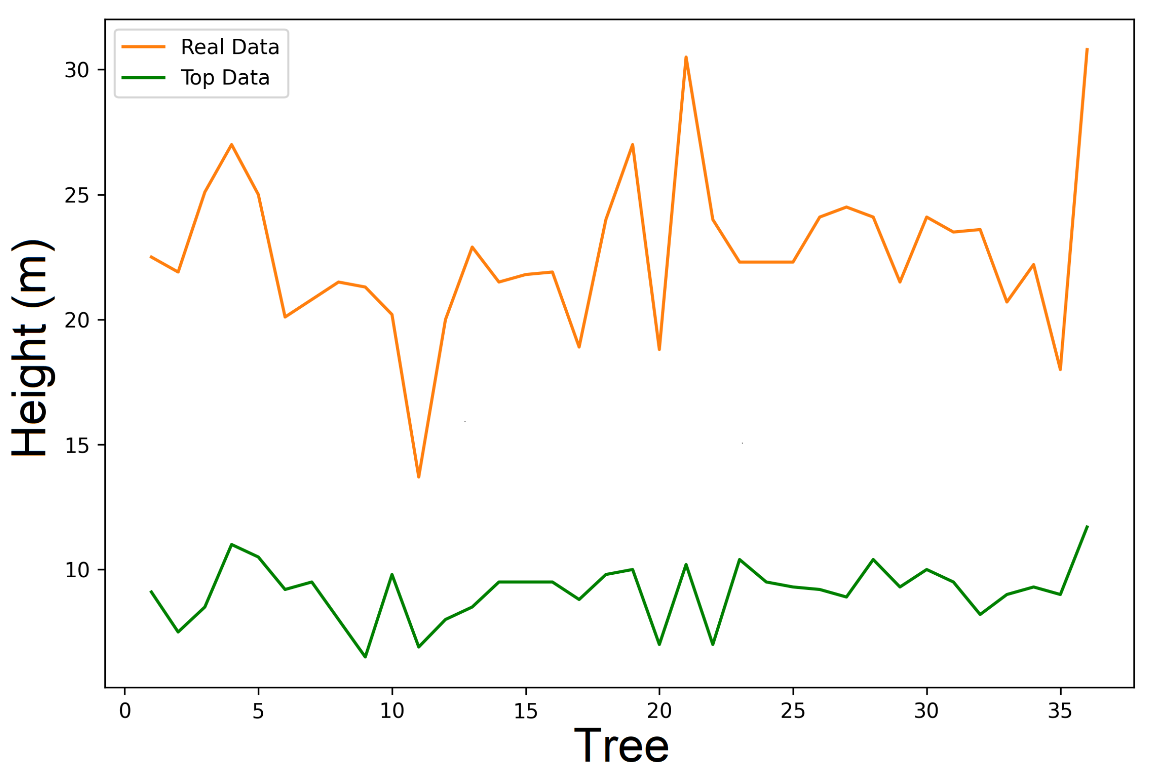
6.2. Real Data

The data consist of observation conducted on 69 trees of the species Pine Radiata distributed in 6 areas. Areas 1, 3 and 5 correspond to a coastal zone, and areas 2, 4 and 6 correspond to interior zones. In each zone, some trees have one disposition NE (dry exposure) and others SW (humid exposure). The method was applied to four sets of data considering the type of exposure and the zone. The first one (Expo1) consists of 36 trees with 8 observations per tree under dry exposure (NE); the second one (Expo2) contains 33 trees with 8 observations per tree under humid exposure (SW). The third set of data consists of 36 trees with 8 observations per tree that correspond to a coastal dry land (Seccos), and the fourth corresponds to an interior dry land (Secint) and contains 33 trees. The method considers some global parameters ($\kappa ,\sigma$, y $\delta$) and some other locals, as in the case of “top height” (${\alpha }_i$). The results for $\kappa ,\sigma$ and $\delta$ are shown in

Table 1. Value parameters.

Zone	$\mathit{\kappa }$	$\mathit{\delta }$	$\mathit{\sigma }$
Expo1	0.1365	0.3538	0.4460
Expo2	0.0930	0.3263	0.4223
Seccos	0.1271	0.3798	0.4221
Secint	0.0830	0.2395	0.4525

, where we can appreciated that the values for $\kappa ,\sigma$ and $\delta$ are slightly better for data of dry exposition 2 and the coastal zone.

The graphics analysis in Figure 15 and Figure 16 shows a comparison of the real height and top height for data of the exposure 1 and exposure 2. The method is slightly better for the data of exposure 2, for which there is an obtaining of a minor variance ($\sigma$ = 0.4223). It is important to point out that the real data of the trees’ height spans eight years; therefore, we must be careful with the interpetation of the graphics. Nevertheless, the tree heights are reasonable. The conclusions obtained in this paper have no difference in comparison with the ones presented by Ratkowski [30] and Seber et al. [8] in relation to Richards model, and independently of the techniques of the estimation used, particulary in the $\delta$ parameter.

7. Conclusions

The field of height growth modelling has predominantly relied on regression-based approaches, often neglecting the explicit modelling of error structures and associated fitting criteria. However, this study presents an innovative approach that views growth trajectories as realisations of a stochastic process. By doing so, it naturally incorporates the error structure into the fitting process, offering a fresh perspective on modelling height growth dynamics. This novel approach utilises Random Time Transformation (RTT) to estimate the parameters of Richards growth model, departing from traditional methods. Unlike classic modelling approaches, the focus here centers on Stochastic Differential Equations (SDE) to characterise growth. The estimation of parameters in Richards growth model has been a challenging endeavor when employing traditional methods. Standard approaches in height growth modelling often struggle to provide accurate parameter estimates due to the inherent complexity of the model and the intricate growth patterns exhibited by real-world data. The primary reasons behind the difficulty in parameter estimation with conventional methods can be attributed to several factors. Firstly, Richards model is known for its flexibility, offering four parameters ($\alpha ,\beta ,\gamma$, and $\delta$) that allow it to fit a wide range of growth patterns. While this flexibility is a strength, it also introduces a significant challenge. The intricate interplay of these parameters necessitates a nuanced and adaptable approach to the estimation. Traditional methods may falter in capturing the nuances of growth when attempting to estimate these parameters. Secondly, the richness and variability of real-world data pose challenges. Growth trajectories of trees are influenced by numerous environmental factors, including soil quality, climate conditions, and competition with neighboring vegetation. These factors introduce variability and complexity that are not always well-captured by standard modelling techniques. The Random Time Transformation (RTT) method is a new approach to parameter estimation in Richards model. It treats growth trajectories as realizations of a stochastic process, which naturally incorporates the error structure into the fitting process. This stochastic formulation aligns with the inherent variability observed in real-world data, making it a valuable tool for parameter estimation. RTT introduces an element of randomness, allowing for the modelling of random environmental variations that influence growth patterns. This adaptability is particularly advantageous when dealing with complex and variable growth dynamics. The method’s sensitivity to changes in variance ($\sigma$) provides insights into the data’s behaviour, aiding in the estimation process. While traditional methods may struggle to provide accurate parameter estimates for the Richards growth model, the RTT method offers a promising alternative. Its stochastic approach, coupled with the modelling of random environmental influences, makes it better suited to capture the intricacies of growth patterns. RTT’s adaptability and sensitivity to variance changes contribute to more reliable parameter estimation, marking a significant step forward in the modelling and understanding of tree growth dynamics. This paradigm shift opens up new possibilities for modelling and understanding growth dynamics with increased flexibility and accuracy. An in-depth analysis of the results sheds light on the sensitivity of RTT to variations in the variance parameter ($\sigma$). Notably, the technique displays some limitations, particularly when $\sigma$ approaches 0.5, rendering it less reliable under such conditions. Concerning the limitations if $\sigma =0.5$, it is necessary to explain that in the context of RTT, $\sigma$ is a crucial parameter that characterises the variance of the random time transformation. When $\sigma =0.5$, it signifies a specific condition where the variance becomes particularly problematic. Here is why this is an issue: when $\sigma$ is precisely 0.5, it implies a particular distribution of time transformations. In this case, the RTT method becomes highly sensitive to changes in this variance. Small variations in the variance can lead to significant fluctuations in the results. This sensitivity makes the method unreliable in such cases. Another problem associated with $\sigma$ = 0.5 is that the likelihood function, which is essential for parameter estimation, becomes unbounded as a function of the $\delta$ parameter when $\delta$ is close to one. This means that as $\delta$ approaches one, the likelihood function increases without a limit, making it challenging to estimate $\delta$ accurately. Additionally, when working with RTT and $\sigma =0.5$, there can be numerical difficulties in finding local minimisers during optimisation. This happens because the form of the likelihood function becomes hard to predict and optimise. The sensitivity to the values of other parameters, such as ${\alpha }_i$, further complicates the optimisation process. Therefore, when $\sigma =0.5$ poses challenges in parameter estimation using RTT, we typically seek alternatives that enhance the method’s reliability and accuracy. This often involves adjusting parameters, exploring alternative models, using hybrid approaches, employing advanced optimisation techniques, and conducting thorough simulation studies to ensure robust results. The choice of alternatives will depend on the specific characteristics of the dataset and research goals.

These insights are drawn from experiments involving real-world data collected from 69 trees across 6 distinct areas, classified as coastal and interior dry land, each experiencing varying levels of sun exposure. The model incorporates both global parameters ($\kappa ,\sigma$, and $\delta$) and local parameters (${\alpha }_i$), providing a comprehensive framework for growth estimation. Consistent with simulations, the variance was found to be approximately 0.42 in both coastal and interior dryland areas. One noteworthy challenge encountered when employing the RTT method is the unbounded nature of the likelihood function concerning the ${\sigma }_i$ parameter, particularly when $\delta$ approaches one. However, when reasonable initial values for $\alpha$ are available, the method demonstrates satisfactory convergence. Additionally, there are instances of numerical complexities when seeking local minimisers due to the unknown form of the likelihood function. The utilisation of the RTT method offers an enticing alternative for modelling tree growth, as it accommodates the influence of random environmental variations on growth dynamics. Ongoing research explores the potential of applying RTT to other time-change processes and compares it with Brownian time. The Random Time Transformation method transcends its initial application in tree growth modelling and finds relevance in a multitude of research domains. Its ability to incorporate stochasticity and random environmental factors into modelling makes it a powerful tool for gaining deeper insights, making predictions, and optimizing processes across diverse fields of study. Furthermore, we are investigating its applicability in diverse fields, including investment finance, option pricing, seismology and structural mechanics, underscoring its versatility and potential for transformative insights. The adaptability of RTT continues to open new avenues for innovative research and problem-solving.

Most published works on height growth modelling are regression-based, but do not explicitly model error structures and use the corresponding fitting criteria. In contrast, there is an approach that takes growth trajectories as realisations of a stochastic process, with the error structure to be used in the fitting process arising naturally out of the stochastic formulation. Thus, the most important contribution of this paper is that for the first time a RTT method has been applied to the estimation of the Richards model, and the focus is based on SDE to model the growth as an alternative to the classic models. The application of the Richards model for estimating growth in a group of trees constitutes a challenge involving estimating the parameters, allowing for greater flexibility. The analysis of the obtained results shows us that the RTT is highly sensitive to changes in the variance. This technique is unreliable for values of $\sigma$ at 0.5. Moreover, the experiments are based on real-life data points of69 trees in 6 areas, which were classified as coastal and interior dry land, with different sun exposure. The model considers some global parameters ($\kappa ,\sigma \mathrm{and}\delta$) and other local (${\alpha }_i$) parameters. We obtained a variance of approximately 0.42 in both areas, which is consistent with the simulations. One difficulty with the RTT method is that the likelihood function is not bounded as a function of the $\delta$ parameter when $\delta$ is close to one. However, the convergence of the method is satisfactory when we have a reasonable starting point for $\alpha$. In some cases, there are numerical difficulties in finding local minimisers, since it is impossible to know the form of the likelihood function. We should also highlight that the method of optimisation used to minimise the likelihood is very sensitive to the values of ${\alpha }_i.$ The use of the RTT method is an attractive alternative for modelling the growth of trees, as it allows for the consideration of the random environmental variation that affects growth. At present, we study the alternative of using it in another time-change process and compare it with the Brownian time. Moreover, we are studying the use of RTT in other types of problems in different fields, for example, investment finance and option price, as well as seismology and structural mechanics.

References

- Delattre, M.; Genon-Catalot, V.; Samson, A. Estimation of Population Parameters in Stochastic Differential Equations with Random Effects in the Diffusion Coefficient. ESAIM Probab. Stat. 2015, 19, 671–688. [Google Scholar] [CrossRef][Green Version]
- Garcí a, O. A Stochastic Differential Equation: Model for the Height Growth of Forest Stand. Biometrics 1983, 39, 1059–1072. [Google Scholar] [CrossRef]
- Garcí a, O.; Ruiz, F. A Growth Model for Eucalypt in Galicia, Spain. For. Ecol. Manag. 2003, 173, 49–62. [Google Scholar] [CrossRef]
- Gushchin, A.; Kuchler, U. Asymptotic Inference for a Linear Stochastic Differential Equation with Time Delay. Bernoulli 1999, 5, 1059–1098. [Google Scholar] [CrossRef]
- Iacus, S. Simulation and Inference for Stochastic Differential Equations with R Examples; Springer Series in Statistics; Springer: New York, NY, USA, 2008. [Google Scholar]
- Kloeden, P.; Platen, E. Numerical Solution of Stochastics Differential Equations; Springer: Berlin/Heidelberg, Germany, 1992. [Google Scholar]
- Kloeden, P.; Platen, E.; Schurz, H.; Sorensen, M. On effects of Discretization on Estimators of Drift Parameters for Diffusion Processes. J. Appl. Probab. 1996, 33, 1061–1076. [Google Scholar] [CrossRef]
- Seber, G.A.E.; Wild, C.J. Nonlinear Regression; John Wiley & Sons, Inc.: Hoboken, NJ, USA, 1989. [Google Scholar]
- Kashyap, R.; Ramachandra Rao, A. Dynamic Stochastic Models from Empirical Data; Academic Press: Cambridge, MA, USA, 1976. [Google Scholar]
- Liang, Y.; Wang, W.; Metzler, R.; Cherstvy, A.G. Anomalous diffusion, nonergodicity, non-Gaussianity, and aging of fractional Brownian motion with nonlinear clocks. Phys. Rev. E 2023, 108, 034113. [Google Scholar] [CrossRef]
- Von Bertalanffy, L. A Quantitative Theory of Organic Growth. Hum. Biol. 1938, 10, 181–213. [Google Scholar]
- Von Bertalanffy, L. Quantitative Laws in Metabolism and Growth. Q. Rev. Biol. 1957, 32, 217–231. [Google Scholar] [CrossRef]
- Richards, F.J. A Flexible Growth for Empirical Use. J. Exp. Bot. 1959, 10, 290–300. [Google Scholar] [CrossRef]
- Aikman, D.P.; Benjamin, L.R. A Model for Plant and Crop Growth, Allowing for Competition for Light by the Use of Potential and Restricted Projected Crown Zone Areas. Ann. Bot. 1994, 73, 185–194. [Google Scholar] [CrossRef]
- Hunt, R. Plant Growth Curves; E. Arnold Publishers: London, UK, 1982; pp. 16–85. [Google Scholar]
- Jorve, E.; Jorve, K. A unified approach to the Richards-model family for use in growth analyses: Why we need only two model forms. J. Theor. Biol. 2010, 267, 417–425. [Google Scholar]
- Larsen, R.U. Plant Grow Modelling by Light and Temperature. Acta Hortic. 1990, 272, 235–242. [Google Scholar] [CrossRef]
- Ramachandra Prasad, T.V.; Krishnamurthy, K.; Kaislam, C. Functional Crop and Cob Growth Models of Maize (Zea mays L.) Cultivars. J. Agron. Crop Sci. 1992, 168, 208–212. [Google Scholar] [CrossRef]
- Fowler, C.W. Density Dependence as Related to Life History Strategy. Ecology 1981, 62, 602–610. [Google Scholar] [CrossRef]
- Sibly, R.M.; Barker, D.; Denham, M.C.; Hone, J.; Pagel, M. On the Regulation of Populations of Mammals, Birds, Fish, and Insects. Science 2005, 309, 607–610. [Google Scholar] [CrossRef]
- Ghosh, H.; Prajneshu. Optimum Fitting of Richards Growth Model in Random Environment. J. Stat. Theory Pract. 2019, 13, 6. [Google Scholar] [CrossRef]
- Dennis, J.E.; Schnabel, R.B. Numerical Methods for Unconstrained Optimization and Nonlinear Equations; SIAM: Philadelphia, PA, USA, 1996. [Google Scholar]
- Jukic, D. Necessary and Sufficient Criteria for the Existence of the Least Squares Estimate for a 3-parametric Exponential Regression Model. Appl. Math. Comput. 2004, 147, 1–17. [Google Scholar]
- Jukic, D.; Scitovski, R. The Best Least Squares Approximation Problem for a 3-parametric Exponential Regression Model, Austral. N. Z. Ind. Appl. Math. J. 2000, 42, 254–266. [Google Scholar]
- White, G.C.; Brishin, I.L. Estimation and Comparison of Parameters in Stochastic Growth Models for Barn Owls. Growth 1980, 44, 97–111. [Google Scholar]
- Bassan, B.; Marcus, R.; Talpaz, H.; Meilijson, I. Parameter Estimation in Diferential Equations, using Random Time Transformation. J. Ital. Statist. Soc. 1997, 2, 77–99. [Google Scholar]
- Adler, R.L.; Shields, P. Skew Products of Bernoulli Shifts with Rotations. Isr. J. Math. 1972, 12, 215–222. [Google Scholar] [CrossRef]
- Alon, N.; Meilijson, I. Random time transformation analysis of Covid19. MedRxiv 2020. [Google Scholar] [CrossRef]
- Lipser, R.; Shiryayev, A. Statistics of Random Process I; Springer: Berlin/Heidelberg, Germany, 1977. [Google Scholar]
- Ratkowsky, D.A. Nonlinear Regression Modeling: A Unified Practical Approach; Marcel Dekker, Inc.: New York, NY, USA, 1983. [Google Scholar]
- Román-Román, P.; Torres-Ruiz, F. A stochastic model related to the Richards-type growth curve.Estimation by means of simulated annealing and variable neighborhood search. Appl. Math. Comput. 2015, 266, 579–598. [Google Scholar]