Improving Data Sparsity in Recommender Systems Using Matrix Regeneration with Item Features

Abstract

With the development of the Web, users spend more time accessing information that they seek. As a result, recommendation systems have emerged to provide users with preferred contents by filtering abundant information, along with providing means of exposing search results to users more effectively. These recommendation systems operate based on the user reactions to items or on the various user or item features. It is known that recommendation results based on sparse datasets are less reliable because recommender systems operate according to user responses. Thus, we propose a method to improve the dataset sparsity and increase the accuracy of the prediction results by using item features with user responses. A method based on the content-based filtering concept is proposed to extract category rates from the user–item matrix according to the user preferences and to organize these into vectors. Thereafter, we present a method to filter the user–item matrix using the extracted vectors and to regenerate the input matrix for collaborative filtering (CF). We compare the prediction results of our approach and conventional CF using the mean absolute error and root mean square error. Moreover, we calculate the sparsity of the regenerated matrix and the existing input matrix, and demonstrate that the regenerated matrix is more dense than the existing one. By computing the Jaccard similarity between the item sets in the regenerated and existing matrices, we verify the matrix distinctions. The results of the proposed methods confirm that if the regenerated matrix is used as the CF input, a denser matrix with higher predictive accuracy can be constructed than when using conventional methods. The validity of the proposed method was verified by analyzing the effect of the input matrix composed of high average ratings on the CF prediction performance. The low sparsity and high prediction accuracy of the proposed method are verified by comparisons with the results by conventional methods. Improvements of approximately 16% based on K-nearest neighbor and 15% based on singular value decomposition, and a three times improvement in the sparsity based on regenerated and original matrices are obtained. We propose a matrix reconstruction method that can improve the performance of recommendations.

1. Introduction

With the development of the Web and the extensive use of various smart devices, people can provide substantial information to the Web in real-time, while simultaneously consuming information. Users who access the Web with the main focus on information consumption face large amounts of available information. The information to which users are exposed contains not only the information they seek, but also spam or a lot of information that they do not want. As users are spending increasing time accessing information they seek on the Web, recommender systems have emerged to provide users with preferred content by filtering large amounts of information, along with providing means of exposing the search results to users more effectively.

Recommender systems generally operate based on collaborative filtering (CF) and content-based filtering (CBF) [1,2,3,4]. CF operates according to memory-based and model-based methods [1,4,5]. Both methods use the user–item matrix, which is a matrix that indicates the preference information evaluated by the user for the item [1,4,5]. The memory-based method first calculates similar users or items in the user–item matrix and applies similar user or item information to predict the user preferences for items to determine recommendation lists [1]. Matrix factorization (MF) is a typical example of the model-based approach [5]. The MF method consists of factorizing the user–item matrix and learning the user propensity based on the decomposed matrix to derive the predictive preference. CBF is a method that involves classifying and recommending users or items by analyzing the user demographic information or item features [4,6,7]. Numerous types of methods exist for CBF, as the available information differs depending on the domain.

The recommendation system is proposed with a variety of approaches, using deep learning as well as MF. First, there is neural collaborative filtering (NCF) model that has developed MF into a deep neural network [8]. There are other methods such as using autoencoder and item2vec [9,10,11]. These approaches leverage dimension reduction or embedding to produce recommendation results. Since deep learning requires the embedding process of user preferences or item information, it is suggested to embed the input matrix as well as to embed item features or similarity of the user and item [12,13]. In addition there are studies using the structure of autoencoder to improve top-k recommendation performance, sequential recommendation, or learning the recommendation structure [14,15,16]. However, these deep neural network based recommendation models do not always provide more precise recommendation results than MF for all situations since the models have a non-linear structure [17].

Recommendation systems offer the advantage of providing appropriate information to users rapidly. However, several disadvantages exist. First, because CF-based recommender systems operate based on information regarding the user using a specific item, such as a user–item matrix, the cold-start problem may exist, which decreases the recommendation reliability when little or no information regarding the user or item is available [18,19]. Moreover, magic-barrier issues may arise when predicting the user preferences based on numerical information, which make it difficult to reflect 100% of the user preferences [20,21]. Accuracy problems are a field of continuous research in recommender systems [1,5,22,23,24]. Problems such as cold-start do not exist in certain CBF approaches as they are not based on the user action history for items such as preferences. However, because CBF operates based on metadata, the recommendation accuracy cannot be guaranteed. That is, the extraction of significant features from various metadata requires a more complex process than CF and it is difficult to ensure the reliability of the predicted user preferences based on the results [4,25,26,27]. We use the advantages of CBF to extract the user preference data and propose a method that can improve existing CF. Thus, we derive a means of improving the existing recommendation accuracy by applying the CBF perspective in CF.

We propose a method for improving the sparseness and increasing the accuracy of the user–item matrix by using item features selected by the users. For this purpose, we apply a hybrid method incorporating CBF and CF. The existing CF method extracts the user information from the user–item matrix (similar users or items for the memory-based approach and latent factors for the model-based approach) and the prediction results are derived. Prior to applying the existing user–item matrix to the CF as input, we regenerate the matrix based on item categories to implement CF.

To achieve this, we first extract the category ratio of the selected items for each user. Thereafter, we apply the extracted information, namely the category ratio, as a filter for the user–item matrix and regenerate the matrix. Therefore, the existing user–item matrix is regenerated based on the category ratio. This regenerated matrix (RM) is assumed to be more user appropriate than the conventional matrix and is applied to the CF. The results are compared with those obtained through the existing matrix. Moreover, we test the sparsity of the regenerated and original matrices, and demonstrate the improvement in the sparsity and accuracy in our approaches. We use the MovieLens dataset (https://grouplens.org/datasets/movielens/, accessed on 26 November 2020) and consider the genre information of the movie as category information in the experiments.

We verify the significance of the RM through various experiments, thereby demonstrating that our approaches are superior compared to the recommendation results derived by conventional CF. Our main research questions can be summarized as follows:

• Can we reconstruct the original input for collaborative filtering to a more dense matrix using user preferences and item features?
• Can the reconstructed matrix alleviate the sparsity problem of the original input?
• Are the results derived through the reconstructed matrix based on various collaborative filtering approaches as accurate as the results of the original matrix?

The remainder of this paper is organized as follows. Related works are introduced in Section 2. The proposed algorithm is presented in Section 3. The experiments and results are detailed in Section 4, and Section 5 provides concluding remarks.

2. Related Work

The recommendation systems based on collaborative filtering approaches can suffer form the cold-start problems and the sparsity issues for the users’ reactions since it operates by utilizing users’ preferences which means reactions for the items. There exist the studies to alleviate the problems in recommender systems by addressing the metadata of the items, such as category information [28,29,30,31,32]. In this section, we introduce and analyze various studies based on collaborative filtering (CF), content-based filtering (CBF), and deep learning approaches to alleviate the cold-start problems, including the sparsity issues in the recommender systems.

2.1. Studies for the Recommendation Systems to Alleviate the Cold-Start Problems

Several studies on hybrid recommender systems have combined methods to overcome the limitations of existing approaches, such as accuracy or cold-start problems. Hybrid recommender systems combine two or more recommendation approaches in different manners, thereby reducing the disadvantages of each method and enhancing each advantage [33]. We focus on hybrid systems addressing collaborative filtering (CF) and content-based filtering (CBF) in various manners.

Various studies have analyzed hybrid recommender systems based on CF and CBF. CBF has been applied not only to e-commerce and e-learning, but also to news recommendation and user preference analysis [33,34,35,36,37]. These approaches utilized item or user features, such as category or demographic information [28,29,30,31,32].

These works addressed the various problems arising from recommender systems [33,38]. Several CBF methods have used item or user features, such as category or demographic information to deal with cold-start problems for new items or new users [28,39,40].

The studies utilize item or a user features in recommendation processes. In other words, items are classified based on the item features such as category and used to derive the recommendation results, or features are used as input from deep neural networks to learn the features together numerical values [8,9]. In addition to this, there is also a method of reconfiguring the input matrix by reusing the results of the MF to improve the performance of the recommendation [41].

Choi and Han [42] proposed a prediction model for new items by using the option of representative users extracted from user rating networks, for which item features, such as category information were utilized. Gantner et al. [43] attempted to cluster new items with no user responses by addressing the feature data. The clustering method based on feature data mitigated the item-side cold-start problem; that is, the authors applied CBF concepts using side information, such as item features to mitigate cold-start in recommender systems. Sun et al. [44] clustered items using the attribute data and preferences, and created a decision tree that could be applied to new and existing items, and could predict preferences for new items. Volkovs et al. [45] combined content- and neighbor-based models, namely CBF and CF, to address the cold-start problem in recommender systems, and their approach produced consistent results in actual testing.

Moreover, studies have been conducted on various hybrid recommender systems to improve the accuracy [6,46,47]. In [6], the authors proposed a Bayesian network model incorporating user, item, and feature nodes. The proposed model was based on a combination of CF and CBF, as it used various features to derive predictions through CF. Superior recommendation quality was provided based on the proposed model. In [47], the authors constructed user features based on the action history of the users, following which the similarities between users and the items (website content) were derived to recommend items.

Meel et al. [48] proposed an approach that could improve the CF accuracy through various analyses of the item features. They analyzed the item features using techniques, such as word2vec and tf–idf, and applied singular value decomposition (SVD) to derive the recommendation results. The item features were analyzed based on the CBF concept and the embedding method was used, which analyzes items through frequency-based methodologies and applies these to CF. Duong et al. [10] generated the tag genome of movie data by applying a natural language processing (NLP) technique. The authors also proposed a three-layer autoencoder to create a more compact representation of the tags. Thereafter, they provided recommendation results by implementing MF. Chen et al. [49] proposed a hybrid recommendation algorithm. They used a latent Dirichlet allocation topic model to reduce the user data dimension and generated a user theme matrix that could reduce the data sparsity for CF. The VGG16 deep learning model was used to extract the feature vectors. The generated matrix and vectors were used as input for content-based recommender systems, following which the recommendation results were derived. Mehrabani et al. [50] proposed a method to extract the item features as words based on the NLP method word2vec. The vectors were used to calculate the similarities between features. After calculating the similarities, the proposed system derived the recommendation results according to the content-based concept.

2.2. Studies for the Recommendation Systems to Improve the Sparsity Issues for Inputs

Recently, various studies related to the improvement of the data sparsity have been conducted [51,52]. These studies are not only attempting to improve based on the existing CF method, but also are being studied based on various methods applying deep learning approaches [52,53,54,55].

In the case of studies that attempt to improve based on the CF method, the features of users or items are used. Zhao et al. [51] proposed a new item-based CF algorithm based on Kullback–Leibler (KL) divergence to measure item similarity. They first try to improve the accuracy of similarity results. Then adjusted prediction results, more rating information is integrated with explicit user preferences in prediction processes. The results of the proposed algorithm show better recommendation quality in the sparsity dataset.

Jiang et al. [53] propose a recommendation model for service API based on knowledge graph and collaborative filtering. They applied latent dimensions in collaborative filtering for analyzing the potential relations between mashups and APIs to reduce the impact of data sparsity. Based on the proposed model, authors have significantly improved the accuracy of service recommendation.

Ahmadian et al. [54] propose a novel recommendation method to address the issues that the existing recommendation methods focused on accuracy of recommendation without the time factor of users. The proposed method first incorporates the temporal issues based on the effectiveness of the users’ rating by utilizing a probabilistic approach. They measure the quality of the prediction with respect to the changes of users’ preferences over time since the proposed method addresses temporal reliability and data sparsity. Through their approaches, the method can remove ineffecive users in the neighbor which means the set of similar users based on the changes of users’ preferences over time. For this step, authors can show the temporal reliability of their recommendation approaches.

Ajaegbu [56] focused on addressing the sparsity and cold-start situations in collaborative filtering by improving the conventional similarity measurements, such as Cosine similarity, Pearson correlation coefficient, and Adjusted cosine similarity. In existing collaborative filtering, by adjusting similarity measurement, author improve the accuracy of recommendation results in sparsity and cold-start situations compared with the results of the conventional similarity measurements.

Khaledian et al. [57] propose trust-based matrix factorization technique (CFMT) that addresses trust network in user data. They utilize the social network data in recommendation processes as trusters and trustees. By using the trust network and integrating ratings and trust statements authors alleviate the sparsity and cold-start problems in a recommendation model.

Zhou et al. [58] propose a hybrid collaborative filtering approaches for consumer service recommendation in mobile cloud using user preferences to deal with the issues for data sparsity and recommendation accuracy. The proposed service recommendation model reduces the sparsity and improves the accuracy of recommendation.

Deep learning-based studies are being conducted using an integrated method of existing CF and neural networks or learning cross-domain. Althbiti et al. [52] propose a novel model based on artificial neural network model CANNBCF (Clustering and Artificial Neural Network-Based Collaborative Filtering) to improve the data sparsity in collaborative filtering. They utilize various domains including books, music, jokes, and movies to evaluate the proposed model. Through the experiments they show that CANNBCF effectively improve the quality of the results for recommendation.

Chen et al. [55] propose attribute-based neural collaborative filtering (ANCF) to improve the approaches that address auxiliary information, such as user/item attributes for sparsity problems in conventional collaborative filtering. The existing approaches deal with the attributes equivalently, whereas the information can differently affect recommendation results. To improve these problems, authors utilize the attention mechanism for integrating and distinguishing the attributes and obtaining complete feature results of user/item. They also use multi-layer perceptron in ANCF for learning non-linear relationships between user/item. Chen et al. show the effectiveness of their approaches through experiments by addressing four publicly available datasets.

Existing models that utilize adversarial learning for cross-domain to alleviate the data sparsity problems in recommendation positively affect side effects for collaborative filtering, such as sparsity problems, however, the models only address the domain-shared features in multiple domains. To leverage not only domain-shared features but also domain-specific knowledge among multiple domains, Liu et al. [59] suggest a novel framework DAAN based on a deep adversarial and attention network. They tried to integrate model-based collaborative filtering, which means matrix factorization with deep adversarial via an attention network. The proposed framework is leveraged to common features in two domains and adjusts the degree of effect between domain-shared and domain-specific knowledge.

Graph collaborative filtering methods that leverage the interaction graph based on users’ preferences for items can positively affect the results of recommendation however, the methods still have side effects, such as data sparsity in real situations. Although there are approaches to reduce the data sparsity using contrastive learning in graph collaborative filtering, the approaches conventionally construct the contrastive pairs ignored for the relationship between users or items. To derive the potential of contrastive learning for recommendation Lin et al. [60] propose a novel contrastive learning approach (NCL-Neighborhood-enriched Contrastive Learning) by addressing different GNN layers for the representations of users and similar groups.

Aljunid et al. [61] propose a neural recommendation model based on non-independent and identically distributed (Non-IID) by integrating explicit and implicit interaction for collaborative filtering. In this study, the explicit interactions are composed of two models; intra and inter couplings using attributes for users and items. Intra-coupled model is leveraged convolutional neural networks and it is integrated with the inter-coupled model. Through the integrated collaborative filtering model, the performance of recommendation is improved.

2.3. Analysis and Motivation

In order to alleviate the cold-start and sparsity problem many studies currently construct and propose a method of predicting users’ preferences for items using information, such as the feature of items [28,29,30,31,32]. In addition, various studies have been conducted to predict users’ evaluation by extracting and analyzing feature vectors of items using deep learning approaches [52,53,54,55]. However, current studies are attempting research that transforms the shape of the existing system using metadata of users or items. Namely, it proposes methods that can produce users’ evaluations in cold-start and sparse situations to produce more accurate results.

The previous studies have the advantage of improving or alleviating the current recommendation performance or the problems of existing recommendation techniques. However, more analysis is required to use the proposed techniques in real situations. For example, in the case of neural collaborative filtering (NCF), a neural network-based recommendation technique, research shows that conventional collaborative filtering approaches, such as matrix factorization produces more accurate results in general situations [17]. The approaches currently being studied can produce more accurate results in specific situations, but have the disadvantage of not having universality, such as conventional collaborative filtering. In addition, the sparsity problems persist since most studies still utilize the same input form [52,53,55]. To overcome these problems, we propose a methodology for reconstructing an input matrix in a form that can alleviate the sparsity problem. We also apply this reconstructed form of input to conventional collaborative filtering approaches by constructing the same structure as the original input, i.e., our approach can be utilized in more versatile situations than related studies and alleviate sparsity problems.

In this paper, we propose a method that can perform data preprocessing by focusing on feature engineering rather than a recommendation method using the metadata of items. There are many studies that produce predictions based on novel recommendation methodologies [28,29,30,52,54,55]. However, if we can re-construct the input matrix by applying the metadata of items, we can derive the recommendation results from existing approaches itself. For example, if different inputs are used in model-based collaborative filtering based on matrix factorization, there is a difference in the prediction results. Similarly, even when different methodologies are applied to the same input, there is a difference in the prediction results. As discussed in this section, the majority of current studies use the view of recommendation techniques rather than the view of changing inputs to alleviate cold-start and sparsity problems.

We propose a method of regenerating the input form rather than the perspective of proposing novel recommendation techniques for alleviating cold-start and sparsity problem. We propose an input reconstruction scheme that can yield more reliable results from the techniques used by many existing e-commerce and content recommendation services. Our approach has the advantage of being able to utilize memory-based and model-based CF approaches that have been commercialized and gained a lot of trust. In addition, the reliability of the method proposed in this paper can be verified by comparing the results derived from the original input form.

3. Our Approach

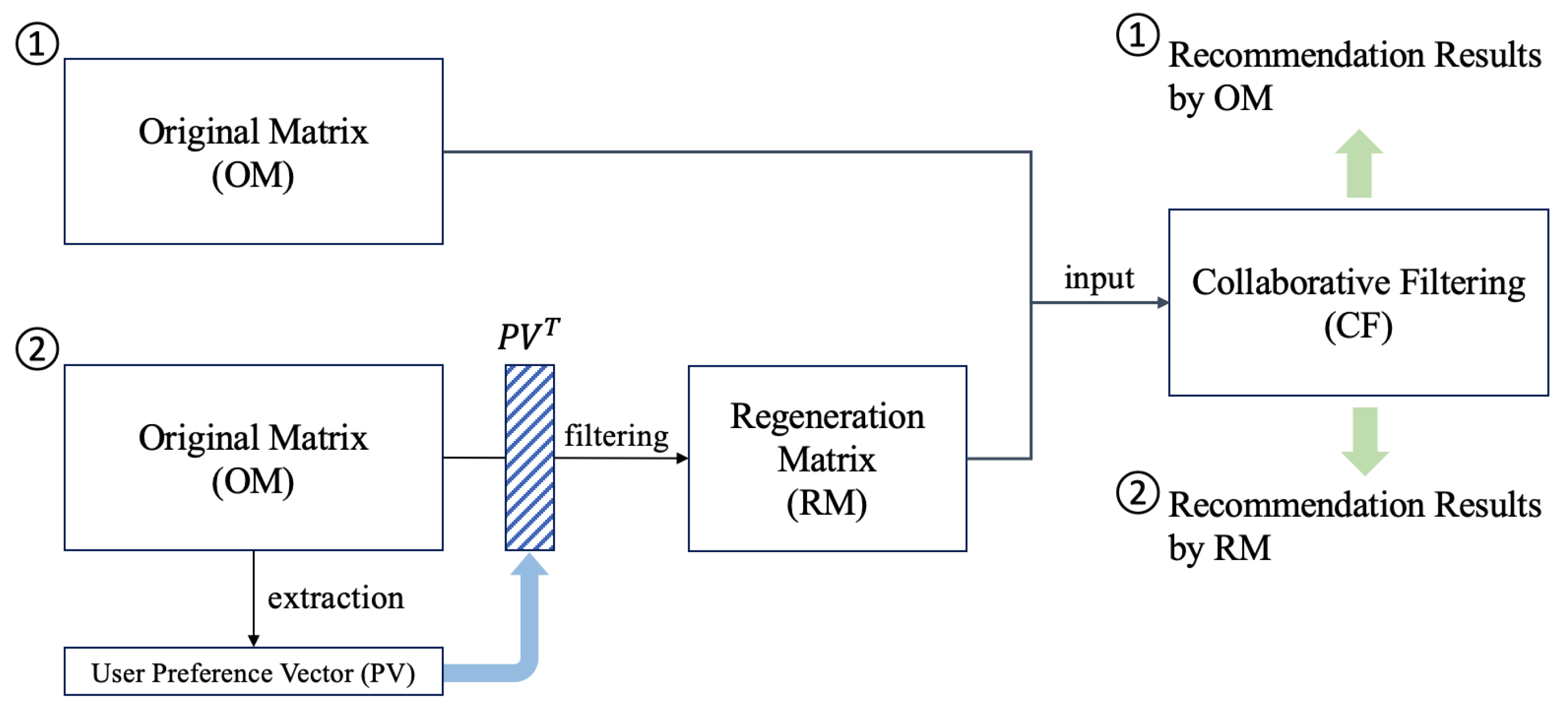
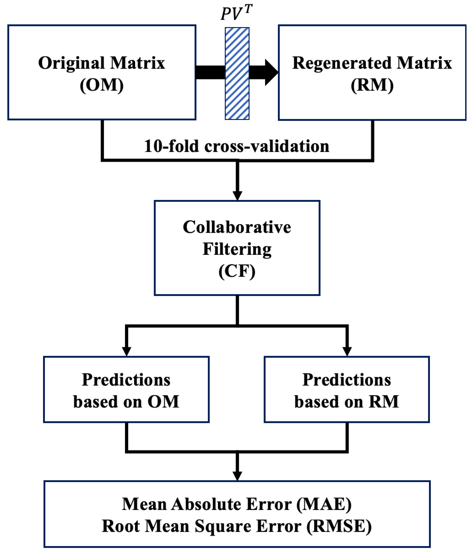
Prior to applying the original matrix (OM) to collaborative filtering (CF), we filter the OM based on the item category information and regenerate the matrix into a more suitable form for the user. In the conventional method, the OM is applied to CF as input and the prediction results are derived. Figure 1 presents the differences between the conventional CF and proposed method. Compared to the conventional CF, we analyze the user selection propensity and extract a matrix that reflects the user preferences from the OM.

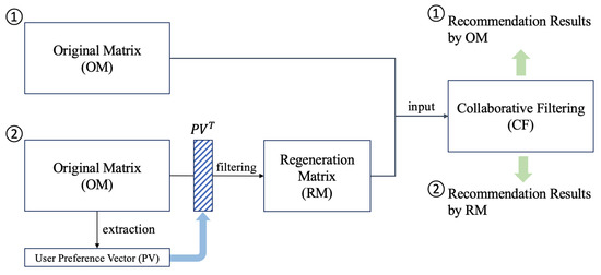
Figure 1. Differences between conventional CF and our approach.

We first extract the category ratio of the selected items by user and regenerate the OM based on the category percentage. The regenerated matrix (RM) is assumed to be more user-appropriate than the OM and is applied to the CF. We conduct experiments using the MovieLens database, and consider the genres that exist in movie information as the category information. Accordingly, we take the movie database as an example to explain the proposed method.

3.1. Database

We employ the MovieLens dataset (https://grouplens.org/datasets/movielens/, accessed on 26 November 2020), as indicated in Table 1, which comprises 9125 movies and 671 users. The movie database provides genre information as an item feature. All movies in the database have at least one genre and each movie has a genre combination. For example, the genres for “Toy Story” are classified as Animation, Children’s, and Comedy. Table 2 presents the 18 genres of the database.

Table 1. MovieLens database.

Dataset	Attribute	Explanation
Movie dataset	MovieID, Title, Genre	A total of 9125 movies
Rating dataset	UserID, MovieID, Rating, Timestamp	A total of 100,004 ratings provided by 671 users

Table 2. 18 genres.

No	Genre	No	Genre
$G_1$	Action	$G_{10}$	Film-Noir
$G_2$	Adventure	$G_{11}$	Horror
$G_3$	Animation	$G_{12}$	Musical
$G_4$	Children’s	$G_{13}$	Mystery
$G_5$	Comedy	$G_{14}$	Romance
$G_6$	Crime	$G_{15}$	Sci-Fi
$G_7$	Documentary	$G_{16}$	Thriller
$G_8$	Drama	$G_{17}$	War
$G_9$	Fantasy	$G_{18}$	Western

3.2. Matrix Regeneration Based on User Preference Filter

Recommendation systems generally use the user–item matrix as an input. The user–item matrix consists of item ratings evaluated by the user. Let $U=u_1,u_2,...,u_n$ be the set of users and $I=i_1,i_2,...,i_m$ be the set of items, where there are n users and m items. Let R be the set of ratings, where $r_{i,j}$ is a rating provided by user $u_i$ for item $i_j$. The user–item matrix is composed of U, I, and R. We consider the user–item matrix as the OM in this study.

We extract the user preference vector (PV) from the OM. Thereafter, we filter the OM using the PV and perform matrix regeneration.

3.2.1. Extracting User PV

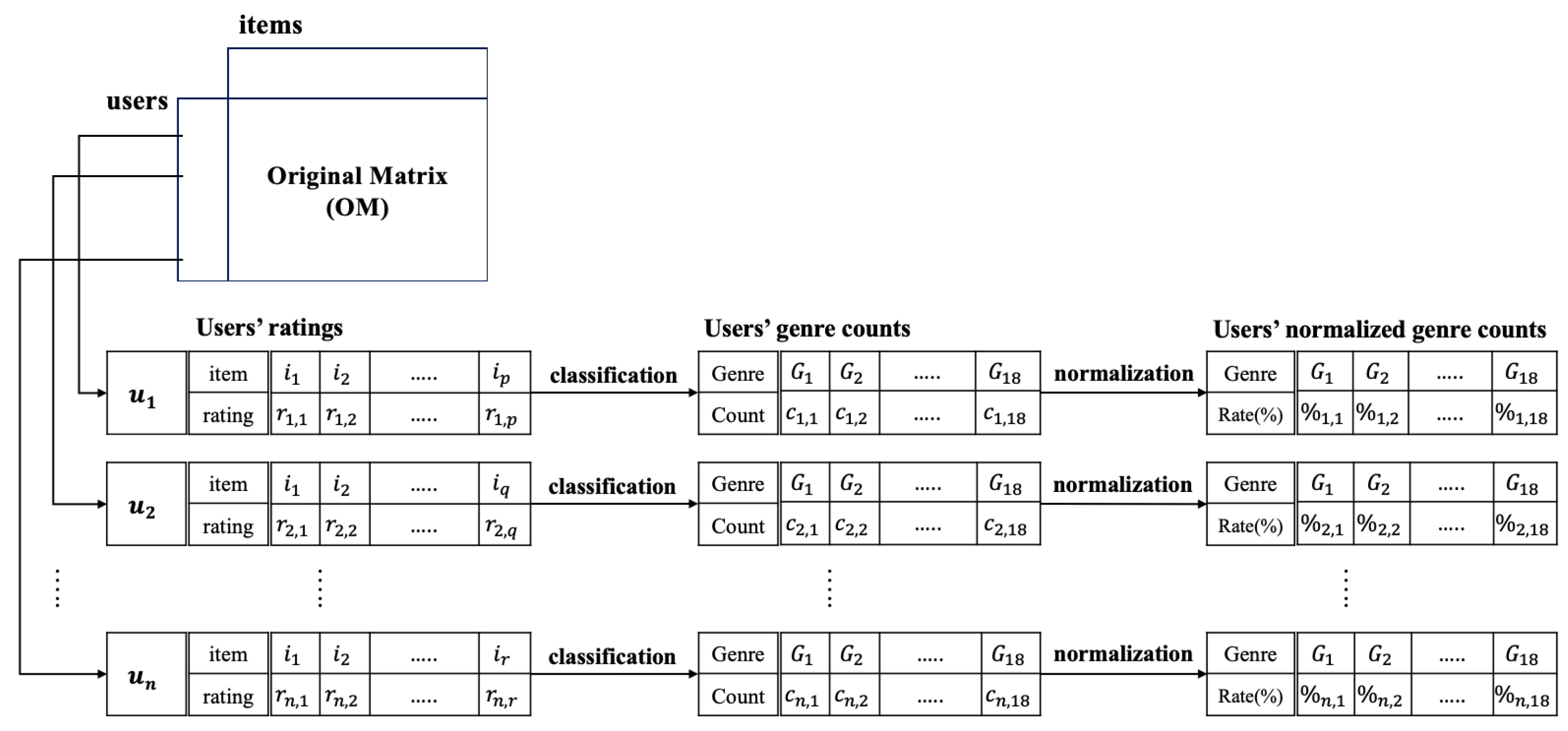
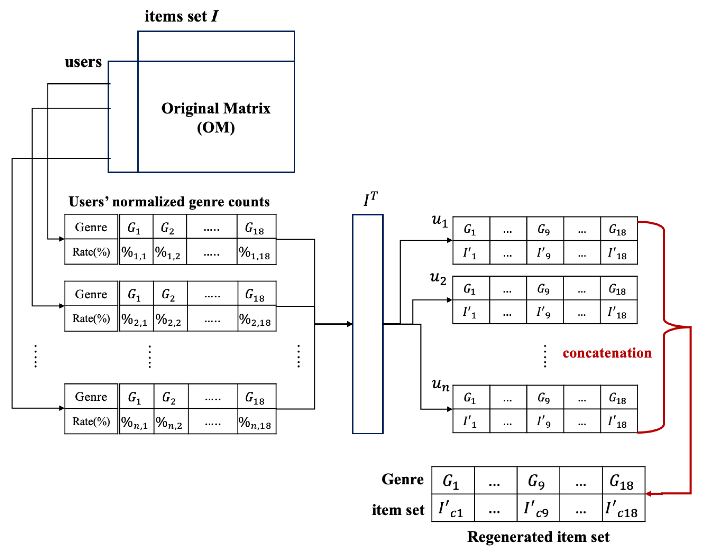
To extract the user PVs, we first extract genres from the items evaluated by users in the OM and calculate the percentage of genres that have been evaluated by users. The item is composed of various features, including the year, actor, genre, and country. We select only the genre among these and calculate the user selection ratio. In a movie, a genre is information selected by a group of experts that can serve as a standard for the characteristics of an item, similar to a category in general e-commerce [28]. A total of 18 genres are included in the MovieLens dataset. Thus, the calculated vectors have a total of 18 dimensions, each with a user-selected ratio for each genre. Figure 2 presents the process of extracting the PVs for each user from the OM.

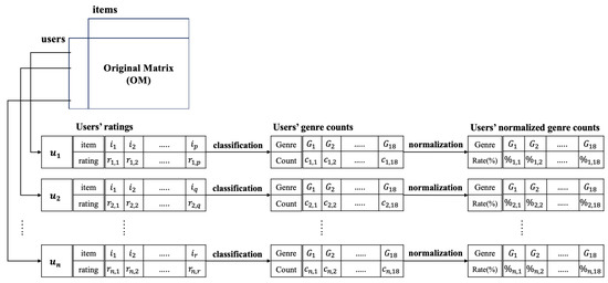
Figure 2. Process of extracting PVs for each user from OM.

In Figure 2, we extract the items that have user preferences, namely ratings, from the OM. For example, in Figure 2, user $u_1$ evaluated a total of q items from items $i_1$ to $i_q$. We count the frequency of the genre appearing in these evaluation items, following which we can obtain vectors for the genre selection frequency by the users. The frequency of genre vectors that exist for each user is below 18 because a total of 18 genres are included in the database. Thus, the maximum number of dimensions is 18; however, certain users may not select a particular genre at all, so the total may be 18 or less. The value of the frequency vector for each user is subsequently calculated through percentile normalization to calculate the user PV.

In Figure 2, assume that users $u_1$ and $u_2$ have the same frequency number for genre $G_1$. However, the value of $G_1$ may differ in each user PV. This is because when the total numbers of frequencies for $G_1$ selected by $u_1$ and $u_2$ are 100 and 20, respectively, $u_1$ has a preference of approximately 10% for $G_1$ and $u_2$ has a preference of 50% for $G_1$.

Normalization is applied to the frequency vectors because, depending on the total number of selected genres, the preference ratio may vary for each user. We derive the PVs taking into account the proportion of the selection-based preferences of these users. Therefore, the preferences can be considered as a percentage of the genre selected by the user.

3.2.2. Matrix Regeneration Using PV

We calculate $GlobalPV$ based on the PV extracted from each user. $GlobalPV$ is derived by calculating the average PV for each user. Equation (1) presents the process of calculating the average rate for a genre in the PV.

$$Av{g}_{G_n}=\frac{{\sum }_{v_i\in U}{v}_i}{\left|U\right|},$$

(1)

where $G_n$ is the $n^{th}$ genre in the dataset, U is a set of users, and $v_i$ is the preference rate of user i for genre $G_n$. Therefore, the result of Equation (1) is the average of the preference rates of all users for genre $G_n$.

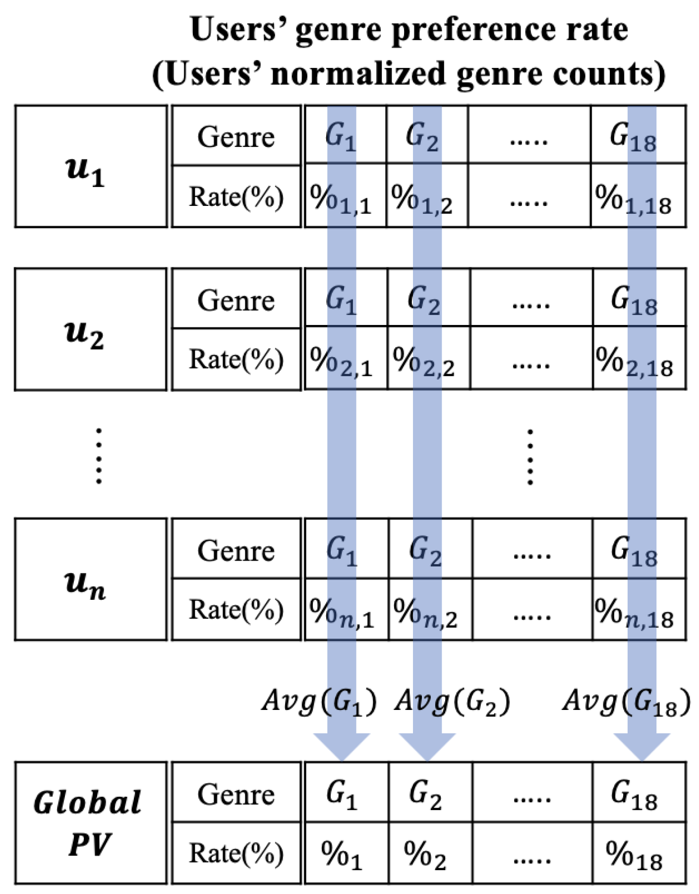
We apply Equation (1) to all genres (from $G_1$ to $G_{18}$) and derive $GlobalPV$. Figure 3 presents the process for deriving $GlobalPV$.

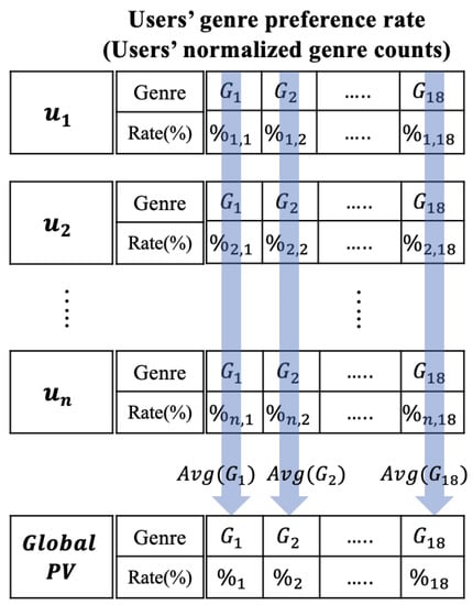
Figure 3. Process for deriving $GlobalPV$.

In Figure 3, a genre preference ratio exists for each user. We derive the average of each column. That is, the average of each genre preference ratio from $G_1$ to $G_{18}$ is calculated in the form depicted in Figure 2 to derive $GlobalPV$.

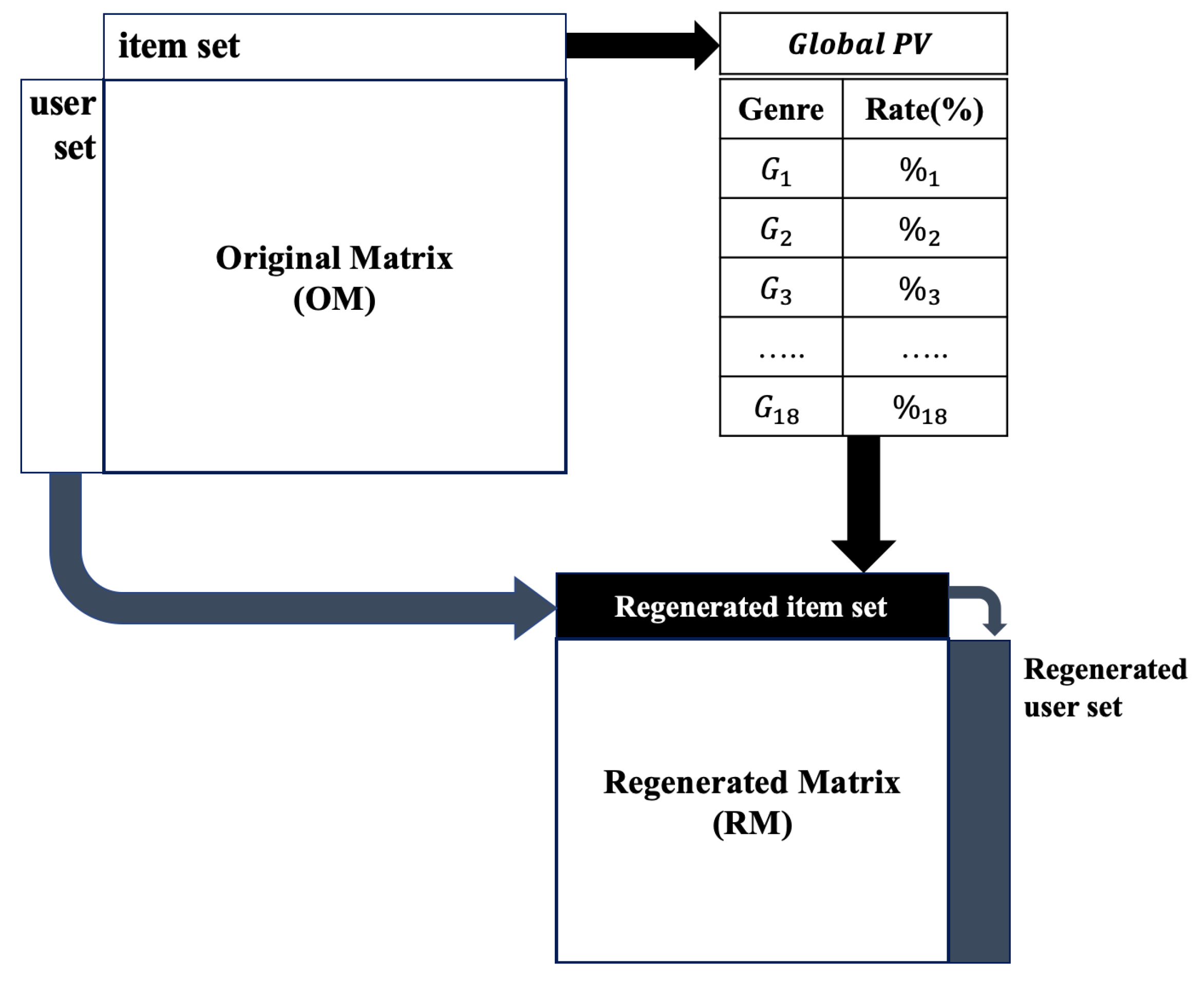
We use $GlobalPV$ to extract a more user-appropriate matrix from the OM. Thus, we consider $GlobalPV$ as a filter and apply it to the OM to regenerate the matrix in which the user preferences are considered. Figure 4 depicts the process of constructing the RM by applying the PV filter to the OM.

Figure 4. Process of constructing RM by applying PV filter to OM.

In Figure 4, for the matrix regeneration, we first classify the items by genre in the OM. Thereafter, we reconstruct the items in the OM based on $GlobalPV$. For example, suppose that there are 100 items in $G_1$ classified from the OM. Assume that the ratio of $G_1$ in $GlobalPV$ is 10%. Based on this ratio, we extract 10, which is 10% of the total of 100 items in $G_1$ of the OM. We apply this to $G_{18}$, and, subsequently, the items to which the genre ratio of $GlobalPV$ is applied are extracted from the OM.

When the set of items in the OM is I and the set of items extracted based on $GlobalPV$ from the OM is $I^{{}^{\prime }}$, $\left|I\right|$≥$|I^{{}^{\prime }}|$. Suppose that a user $u_a$ has evaluated all items in the OM. When the set of items extracted from the OM based on $PV$ for $u_a$ is $I_a$, $\left|I\right|=|I_a|$. In all cases except this, $\left|I\right|>|I^{{}^{\prime }}|$.

Thereafter, all users who evaluated the set of items $I^{{}^{\prime }}$ are extracted. If the set of users existing in the OM is U and the set of users extracted based on $I^{{}^{\prime }}$ from the OM is $U^{{}^{\prime }}$, $\left|U\right|$≥$|U^{{}^{\prime }}|$. In the extracted user set, similar to the item set, $\left|U\right|$=$|U^{{}^{\prime }}|$ for users who have evaluated all items. For all cases except this, $\left|U\right|$>$|U^{{}^{\prime }}|$.

We extract all users who have evaluated the extracted item set $I^{{}^{\prime }}$. Suppose that the set of users extracted based on $I^{{}^{\prime }}$ is $U^{{}^{\prime }}$. Then, we can construct a new matrix $RM$ using $I^{{}^{\prime }}$ and $U^{{}^{\prime }}$.

4. Experiments

We applied the regenerated matrix (RM) and original matrix (OM) to collaborative filtering (CF), and analyzed the results. Figure 5 presents the entire experimental process. In our experiments, we do not provide the environments for experiments since our approaches including collaborative filtering have no real-time issue. Because of this reason, we show the experimental process and the results of our test. We first describe the CF approaches utilized for our experiments. Then we provide and analyze the experimental results using RM and OM as input for each CF approach.

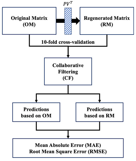
Figure 5. Experimental process.

We first introduce the CF methods used in the experiment. Thereafter, we present the experimental design and the method used to compare the results. Finally, the results and analyses are provided. We used the mean absolute error (MAE) and root mean square error (RMSE) to verify the accuracy in the experiments. We calculated the sparsity of the input matrices and analyzed the results. Moreover, the differentiation of the results was verified through the Jaccard similarity of the set items in each matrix.

4.1. CF Approaches Used in Experiments

We leverage the conventional CF approaches that utilize various applications in real-services for the experiments. The conventional CF can be divided into memory-based and model-based methods. The memory-based approach is considered as being neighborhood based, and provides a method of identifying similar users and using them to derive recommendation results [1]. Model-based methods are considered as latent factor models and are represented by matrix factor models [5]. We applied the RM and OM to both types of methods to compare the results. The following CF approaches were used in the experiments:

4.1.1. K-Nearest Neighbor (KNN) Approaches

KNN approaches [62] measure the similarity between users or items in the OM and select a similar user or item. The selected similar users or items are referred to as neighbors. Cosine similarity [1] or the Pearson correlation coefficient [63] is used to calculate the similarity. The similarity calculations can be carried out on a user or an item basis. In this paper, the process is explained on a user basis.

After selecting a similar user, namely a neighbor, the prediction results are calculated based on the existing ratings of the neighbor. We used the following four prediction methods for the experiments in this study.

• KNN (Basic): this method obtains the prediction results through the weighted average of the neighbor ratings, for which we use Equation (2).

  $${\widehat{r}}_{u,i}=\frac{{\sum }_{v\in N_i^k\left(u\right)}^{}sim(u,v)·r_{vi}}{{\sum }_{v\in N_i^k\left(u\right)}^{}sim(u,v)},$$

  (2)

  where u is a user and i is an item to predict for u. Furthermore, N is a set of similar users to user u, so v is one of the similar users as an element of the set N, $sim(u,v)$ indicates the similarity between users u and v, and $r(v,i)$ is a rating for item i by user v.
• KNN (Means): this method obtains the prediction results by considering the average of the neighbor ratings, for which we use Equation (3).

  $${\widehat{r}}_{u,i}=\mu \left(u\right)+\frac{{\sum }_{v\in N_i^k\left(u\right)}^{}sim(u,v)·(r_{vi}-\mu \left(v\right))}{{\sum }_{v\in N_i^k\left(u\right)}^{}sim(u,v)},$$

  (3)

  where $\mu \left(u\right)$ is the average rating of user u. The other variables are the same as in Equation (2).
• KNN (Zscore): this method obtains the prediction results by considering the z-score normalization of the neighbor ratings, for which we use Equation (4).

  $${\widehat{r}}_{ui}=\mu \left(u\right)+{\sigma }_u\frac{{\sum }_{v\in N_i^k\left(u\right)}^{}sim(u,v)·(r_{vi}-\mu \left(v\right))/{\sigma }_v}{{\sum }_{v\in N_i^k\left(u\right)}^{}sim(u,v)},$$

  (4)

  where ${\sigma }_u$ and ${\sigma }_v$ are the standard deviations for the average ratings of users u and v, respectively. The other variables are the same as in Equation (3).
• KNN (Baseline): this method is similar to KNN (Means); however, it uses the baseline instead of the average and adds the baseline to a user. For this purpose, we use Equation (5).

  $${\widehat{r}}_{u,i}=b_{u,i}+\frac{{\sum }_{v\in N_i^k\left(u\right)}^{}sim(u,v)·(r_{vi}-b_{v,i})}{{\sum }_{v\in N_i^k\left(u\right)}^{}sim(u,v)},$$

  (5)

  where $b_{u,i}$ and $b_{v,i}$ are the baselines of users u and v, respectively, and $b_{u,i}$ is defined by Equation (6).

  $${\widehat{r}}_{u,i}=b_{u,i}=\mu +b_u+b_i,$$

  (6)

  where $\mu$ is the global average rating of the OM, and $b_u$ and $b_i$ are the bias (or baseline) for the user and item, respectively.

4.1.2. MF Approaches

MF [64] determines the values of the decomposed matrix through learning in the process of factoring and recombining the user–item matrix; that is, the input matrix. In this case, it is known as a latent factor model, as the intentions of the users or items can be understood in the process of identifying the decomposed matrix. The prediction results are derived through the process of adding these latent factors. We used two MF approaches, namely SVD and non-negative MF (NMF), in this paper. SVD and NMF both use stochastic gradient descent for learning.

• SVD: this is one methodology of MF and can be expressed in the form of $R=U\Sigma V^T$. In this case, R is the input matrix, U is a matrix of size $m\times m$, $\Sigma$ is a matrix of size $m\times n$ with a non-diagonal component of 0, and V is the matrix $n\times n$. This constitutes probabilistic MF and the prediction results are derived through Equation (7).

  $${\widehat{r}}_{u,i}=\mu +b_u+b_i+q_i^T{p}_u,$$

  (7)

  where $\mu$ is the global average rating, $b_u$ and $b_i$ are the bias of the user and item, respectively, and $q_i$ and $p_u$ are the latent vectors for the item and user, respectively.
• NMF: This method is similar to SVD, and we use Equation (8) to derive the prediction results.

  $${\widehat{r}}_{u,i}=q_i^T{p}_u$$

  (8)

4.2. Experimental Design

We conducted the experiments using the database introduced in Table 1. Three methods were used as the basis for item composition in the process of reconstructing the matrix, as follows:

• Selection based (RM-1): a method of extracting items in the order of user selection in the matrix reconstruction. Figure 6 presents the selection-based matrix reconstruction.
  

  Figure 6. Process of selection-based matrix reconstruction.
  For example, in Figure 6, $GlobalPV$ has 10% of $G_1$. Suppose that $G_1$ has a total of 100 items in the OM. Then, we sort the 100 items in descending order based on the user selection frequency. Thereafter, we extract the top 10 items from the sorted items and select the items of $G_1$ in the RM.
• Average based (RM-2): a method of extracting items in the order of the average user ratings in the matrix reconstruction. Figure 6 depicts the average-based matrix reconstruction.
  Figure 7 is similar to Figure 6 except for the item selection process. For example, the difference is that $G_1$ items in the OM are sorted in descending order based on the average rating. We applied this process to all genres.
  

  Figure 7. Process of average-based matrix reconstruction.
• Random based (RM-3): a method of extracting items randomly according to the ratio of $GlobalPV$ in the matrix reconstruction.

We selected RM-1 and RM-2 as the proposed methods for the RM composition. For comparison testing, RM-3 was added, with random extraction at a rate of $GlobalPV$ used by RM-1 and RM-2. The comparative experiments with RM-3 demonstrated the significance of RM-1 and RM-2. We conducted the experiments with RM-1, RM-2, and RM-3 as the CF input.

Moreover, for further comparative experiments, the OM and the following method were used as the CF input.

• Method for comparative experiments: we extracted the user-level RM ($r{m}_u$) and concatenated the matrices, based on which the CF results were derived. The concatenated matrix was the result of adding the items ($I_u^{{}^{\prime }}$) of $r{m}_u$ derived from each user. The set of items in $R{M}_c$ could be considered as a result of combining the genre preferences of each user in the OM. The difference from $RM$ extracted through the $GlobalPV$ filter was the result of considering the average genre preferences of the OM users in the case of $RM$ and $R{M}_c$ was the result of adding the genre preferences of each user. Figure 8 depicts the process of generating $R{M}_c$. We used two methods for each user $r{m}_u$, namely the selection-based and average-based methods, as in the case of deriving $RM$.
  

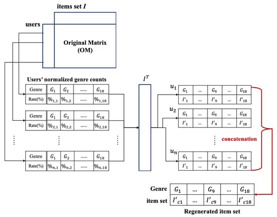  Figure 8. Process of generating $R{M}_c$.

Table 3 summarizes the matrices used as the CF input in the experiments.

Table 3. Matrices used in experiments.

Method		Description
Average genre rate	RM-1	Results of applying GlobalPV to OM, consisting of an item set based on user selection frequency
	RM-2	Results of applying GlobalPV to OM, consisting of an item set based on high user average preference
	RM-3	Results of applying GlobalPV to OM, consisting of an item set based on random selection
Total genre rate	RMc-1	Results of concatenating each $r{m}_u$, consisting of an item set based on high user selection frequency
	RMc-2	Results of concatenating each $r{m}_u$, consisting of an item set based on high user average preference
	OM	Original Matrix, namely user–item matrix

We used the MAE and RMSE to compare the accuracy of the methods. Equations (9) and (10) express the MAE and RMSE, respectively.

$${\displaystyle MAE=\frac{1}{\left|T\right|}\sum _{n\in T}|r_n-{\widehat{r}}_n|,}$$

(9)

$$RMSE=\sqrt{{\displaystyle \frac{1}{\left|T\right|}\sum _{n\in T}(r_n-{\widehat{r}}_n{)}^2}},$$

(10)

where T is the test set of items and n is one of the test items. Furthermore, $r_n$ and ${\widehat{r}}_n$ denote the real rating and predicted rating for item n, respectively.

For a more precise and varied analysis, we divided the test set using 10-fold cross-validation [63,65,66] for each matrix and conducted experiments to derive the MAE and RMSE results. In general, if we use k-fold cross-validation for the experiments, more reliable experimental results can be provided based on a small set of data. In this paper, we conducted an experiment using 10-fold cross-validation to provide more reliable experimental results on a limited size dataset. In total, 10 experimental results can be provided for the same input, which is derived from different test sets. That is, we can derive 10 different test results from the same input through 10-fold cross-validation. We utilize 10-fold cross-validation to derive more experimental results from limited input data.

4.3. Experimental Results

4.3.1. Analysis of Accuracy

Table 4 shows the CF methods used in our experiments and its ID. These IDs are utilized in Table 5 and Table 6. Table 5 and Table 6 display the results of the 10-fold cross-validation with each CF approach. In the tables, $Fold-n$ indicates each dataset for the 10-fold cross-validation, whereas $Mean$ and $St.dev.$ denote the average and standard deviation of the MAE for each dataset, respectively.

Table 4. CF method and ID.

ID	Method
1	KNN (Basic)
2	KNN (Baseline)
3	KNN (Means)
4	KNN (Zscore)
5	SVD
6	NMF

Table 5. MAE results for 10-fold cross-validation with each CF approach.

ID	Method	Fold 1	Fold 2	Fold 3	Fold 4	Fold 5	Fold 6	Fold 7	Fold 8	Fold 9	Fold 10	Mean	St. Dev.
1	RM-1	0.7006	0.6897	0.703	0.7036	0.7008	0.6962	0.7048	0.6914	0.6997	0.6936	0.6983	0.005
	RM-2	0.5982	0.6297	0.6177	0.6088	0.6239	0.6249	0.6149	0.6259	0.6425	0.6396	0.6226	0.0127
	RM-3	0.8052	0.8004	0.8307	0.837	0.7935	0.8164	0.8059	0.8022	0.8151	0.8195	0.8126	0.0131
	RMc-1	0.6984	0.7134	0.7159	0.7086	0.69	0.7035	0.6992	0.7015	0.7108	0.7097	0.7051	0.0076
	RMc-2	0.6249	0.6453	0.6366	0.6007	0.6224	0.6365	0.6034	0.6382	0.6222	0.6206	0.6251	0.014
	OM	0.7419	0.7393	0.7424	0.7392	0.7319	0.7419	0.7369	0.7339	0.7382	0.7407	0.7386	0.0033
2	RM-1	0.66	0.6617	0.66	0.6614	0.6554	0.6573	0.6518	0.6556	0.6545	0.6535	0.6571	0.0033
	RM-2	0.5881	0.5765	0.5726	0.6018	0.5725	0.5923	0.5911	0.5879	0.5855	0.577	0.5845	0.0091
	RM-3	0.7399	0.7357	0.7469	0.746	0.7447	0.7438	0.7364	0.7504	0.7321	0.7514	0.7427	0.0061
	RMc-1	0.6698	0.6607	0.6679	0.6627	0.6604	0.671	0.6539	0.6559	0.6604	0.6501	0.6613	0.0065
	RMc-2	0.6063	0.5878	0.6008	0.5781	0.5803	0.5755	0.5807	0.584	0.5834	0.5954	0.5872	0.0098
	OM	0.6904	0.6903	0.6871	0.6767	0.6801	0.6844	0.6764	0.6768	0.6883	0.6787	0.6829	0.0055
3	RM-1	0.6679	0.665	0.669	0.6779	0.6787	0.6564	0.6622	0.6794	0.6489	0.6622	0.6668	0.0095
	RM-2	0.5752	0.5762	0.5865	0.5981	0.5935	0.5851	0.6021	0.6035	0.5715	0.5883	0.588	0.0108
	RM-3	0.7395	0.753	0.7618	0.7441	0.7736	0.7803	0.7672	0.7693	0.756	0.7549	0.76	0.0123
	RMc-1	0.6733	0.6575	0.6746	0.671	0.6722	0.6794	0.6758	0.678	0.6708	0.6722	0.6725	0.0057
	RMc-2	0.5865	0.5954	0.5888	0.5817	0.5743	0.5634	0.6122	0.5844	0.5929	0.5917	0.5871	0.0123
	OM	0.6879	0.6933	0.6957	0.7059	0.693	0.7049	0.7058	0.7094	0.6924	0.7049	0.6993	0.0072
4	RM-1	0.6627	0.6697	0.6737	0.6606	0.6618	0.6579	0.6559	0.6568	0.683	0.6573	0.6639	0.0084
	RM-2	0.599	0.5855	0.5919	0.593	0.6028	0.5987	0.5814	0.5936	0.5766	0.5773	0.59	0.0088
	RM-3	0.7696	0.7352	0.7609	0.77	0.7794	0.7608	0.7498	0.7364	0.7397	0.7519	0.7554	0.0145
	RMc-1	0.6792	0.6659	0.6626	0.6647	0.669	0.6824	0.6737	0.6658	0.6593	0.67	0.6693	0.0069
	RMc-2	0.5843	0.5712	0.5795	0.569	0.5845	0.5949	0.6012	0.614	0.5869	0.6033	0.5889	0.0137
	OM	0.6846	0.6951	0.6928	0.6951	0.693	0.7002	0.7017	0.7055	0.6957	0.6949	0.6959	0.0054
5	RM-1	0.6595	0.6625	0.6663	0.6459	0.6661	0.6705	0.6705	0.6714	0.6658	0.6729	0.6651	0.0075
	RM-2	0.5825	0.5811	0.5873	0.5843	0.5753	0.5898	0.5791	0.5887	0.5889	0.5927	0.585	0.0052
	RM-3	0.6964	0.7344	0.7024	0.7217	0.7351	0.72	0.7154	0.7049	0.7188	0.7105	0.716	0.0122
	RMc-1	0.6616	0.6588	0.6784	0.6645	0.667	0.6638	0.6719	0.6754	0.6792	0.6722	0.6693	0.0068
	RMc-2	0.5696	0.5951	0.5735	0.5923	0.6	0.5719	0.585	0.5878	0.5644	0.5612	0.5801	0.0129
	OM	0.6823	0.6865	0.6851	0.6834	0.6854	0.6791	0.6922	0.6886	0.7052	0.6817	0.6869	0.007
6	RM-1	0.6751	0.6777	0.6863	0.6868	0.6951	0.6737	0.6939	0.6944	0.687	0.6815	0.6852	0.0075
	RM-2	0.6577	0.6443	0.6285	0.631	0.6566	0.6349	0.6394	0.6241	0.6352	0.6327	0.6384	0.0107
	RM-3	0.8112	0.8168	0.8039	0.7865	0.8283	0.8169	0.8084	0.8002	0.7983	0.7946	0.8065	0.0117
	RMc-1	0.7005	0.6916	0.69	0.6918	0.6918	0.7017	0.69	0.6894	0.7011	0.6914	0.6939	0.0048
	RMc-2	0.641	0.6434	0.6375	0.6414	0.6375	0.6351	0.6336	0.6409	0.6311	0.647	0.6389	0.0046
	OM	0.713	0.726	0.7285	0.7125	0.723	0.7276	0.7311	0.7132	0.7196	0.7254	0.722	0.0066

Table 6. RMSE results for 10-fold cross-validation with each CF approach.

CF	Method	Fold 1	Fold 2	Fold 3	Fold 4	Fold 5	Fold 6	Fold 7	Fold 8	Fold 9	Fold 10	Mean	St. Dev.
1	RM-1	0.907	0.9082	0.918	0.9167	0.9139	0.9156	0.9206	0.9013	0.9129	0.9017	0.9116	0.0064
	RM-2	0.7786	0.8113	0.8051	0.8012	0.8104	0.8315	0.7994	0.825	0.8526	0.8327	0.8148	0.02
	RM-3	1.0278	1.0408	1.0689	1.08	1.0393	1.0572	1.0494	1.0399	1.0506	1.0597	1.0514	0.0148
	RMc-1	0.9152	0.9313	0.941	0.9274	0.9004	0.9202	0.9107	0.9106	0.9178	0.9304	0.9205	0.0115
	RMc-2	0.8195	0.8493	0.8339	0.7792	0.815	0.8368	0.7805	0.8449	0.8108	0.8186	0.8188	0.023
	OM	0.963	0.9666	0.9663	0.9563	0.9516	0.9693	0.9548	0.952	0.963	0.9704	0.9613	0.0067
2	RM-1	0.868	0.8688	0.8631	0.868	0.8539	0.8607	0.8528	0.8593	0.8573	0.8564	0.8608	0.0056
	RM-2	0.7833	0.7444	0.7452	0.7887	0.7564	0.7889	0.7773	0.7783	0.7634	0.7628	0.7689	0.016
	RM-3	0.9644	0.973	0.9759	0.9684	0.9587	0.9628	0.9575	0.9803	0.949	0.9813	0.9671	0.01
	RMc-1	0.8681	0.8731	0.8712	0.873	0.8649	0.879	0.8616	0.8596	0.8607	0.8455	0.8657	0.009
	RMc-2	0.7997	0.7768	0.781	0.766	0.7563	0.767	0.7561	0.7785	0.7689	0.7808	0.7731	0.0124
	OM	0.9092	0.8989	0.8957	0.8825	0.8838	0.8944	0.8863	0.8836	0.8986	0.8862	0.8919	0.0084
3	RM-1	0.8787	0.8691	0.8709	0.8835	0.8823	0.8607	0.8699	0.8866	0.8541	0.8685	0.8724	0.0098
	RM-2	0.7557	0.7487	0.7843	0.7807	0.7798	0.7592	0.797	0.8091	0.7569	0.7702	0.7741	0.0186
	RM-3	0.9508	0.982	1.0008	0.9739	1.0253	1.0122	1.0139	1.0091	0.9817	0.9881	0.9938	0.0214
	RMc-1	0.8714	0.8614	0.8778	0.8768	0.8828	0.8836	0.8822	0.8874	0.8765	0.8847	0.8785	0.0072
	RMc-2	0.7772	0.7847	0.7706	0.7687	0.76	0.7379	0.7924	0.7818	0.7742	0.794	0.7742	0.0157
	OM	0.8969	0.9096	0.9077	0.9193	0.9114	0.9206	0.9202	0.9243	0.9076	0.92	0.9138	0.0081
4	RM-1	0.8691	0.8747	0.8822	0.8698	0.881	0.866	0.8606	0.8644	0.8943	0.8629	0.8725	0.01
	RM-2	0.8082	0.7793	0.7942	0.7718	0.7855	0.8009	0.7617	0.785	0.7623	0.7605	0.7809	0.0161
	RM-3	1.0049	0.9592	0.9906	1.0203	1.015	0.9951	0.9906	0.9742	0.9745	0.9986	0.9923	0.018
	RMc-1	0.892	0.8763	0.8711	0.8732	0.8795	0.8931	0.8807	0.8784	0.8657	0.882	0.8792	0.0081
	RMc-2	0.7751	0.7657	0.7829	0.7408	0.7635	0.7981	0.797	0.8039	0.7864	0.7998	0.7813	0.0191
	OM	0.8959	0.9158	0.9126	0.9109	0.914	0.9163	0.9194	0.9286	0.9162	0.9155	0.9145	0.0077
5	RM-1	0.8594	0.8631	0.865	0.8406	0.8769	0.8755	0.8762	0.8759	0.8709	0.8769	0.868	0.011
	RM-2	0.7576	0.766	0.773	0.7639	0.768	0.7715	0.7562	0.7697	0.7804	0.7917	0.7698	0.01
	RM-3	0.9046	0.9413	0.9077	0.9183	0.9474	0.9235	0.929	0.9113	0.9369	0.9194	0.9239	0.0138
	RMc-1	0.8681	0.8596	0.8867	0.8592	0.8666	0.8617	0.8768	0.8789	0.8866	0.8845	0.8729	0.0106
	RMc-2	0.7495	0.7836	0.7625	0.7733	0.7884	0.7708	0.7758	0.7684	0.7225	0.7348	0.763	0.0201
	OM	0.8827	0.8901	0.8907	0.8904	0.8883	0.8813	0.8988	0.8999	0.9175	0.8856	0.8925	0.0101
6	RM-1	0.8802	0.8847	0.8952	0.8939	0.9155	0.8732	0.9024	0.9073	0.9037	0.8944	0.8951	0.0123
	RM-2	0.8475	0.831	0.8115	0.8118	0.851	0.8269	0.8332	0.7962	0.8212	0.823	0.8253	0.0158
	RM-3	1.041	1.053	1.0382	1.0188	1.0666	1.0534	1.048	1.0322	1.0315	1.0307	1.0413	0.0133
	RMc-1	0.9143	0.8977	0.8956	0.8992	0.9049	0.9166	0.8977	0.9104	0.9148	0.8955	0.9047	0.0082
	RMc-2	0.8371	0.8371	0.8199	0.824	0.8289	0.8329	0.8269	0.8301	0.8096	0.8395	0.8286	0.0086
	OM	0.9322	0.9395	0.9483	0.9267	0.9422	0.9538	0.9493	0.9349	0.9315	0.9475	0.9406	0.0086

It can be observed from Table 5 that the MAE of RM-2 in almost all folds, namely in each dataset, was better than those of the other matrices. Moreover, RM-1 exhibited superior results in our approaches. In the $Mean$ column, RM-1 and RM-2 exhibited superior results to the OM, which means that our approaches could derive better prediction results. In comparison, the results of RM-3 were more inaccurate than those of the OM. Thus, the extraction methods of RM-1 and RM-2 were significant. Moreover, RMc-1 and RMc-2 exhibited better performance than the OM, but were worse than RM-1 and RM-2, respectively.

In Table 5, from the perspective of each CF approach, it can be observed that RM-1 and RM-2 still derived more accurate results than the OM. Among the four KNN approaches, RM-2 exhibited the best performance, and the same results were achieved by SVD and NMF, which are MF approaches. Thus, RM-1 and RM-2 yielded higher accuracy in all methodologies than the results derived from the OM as input.

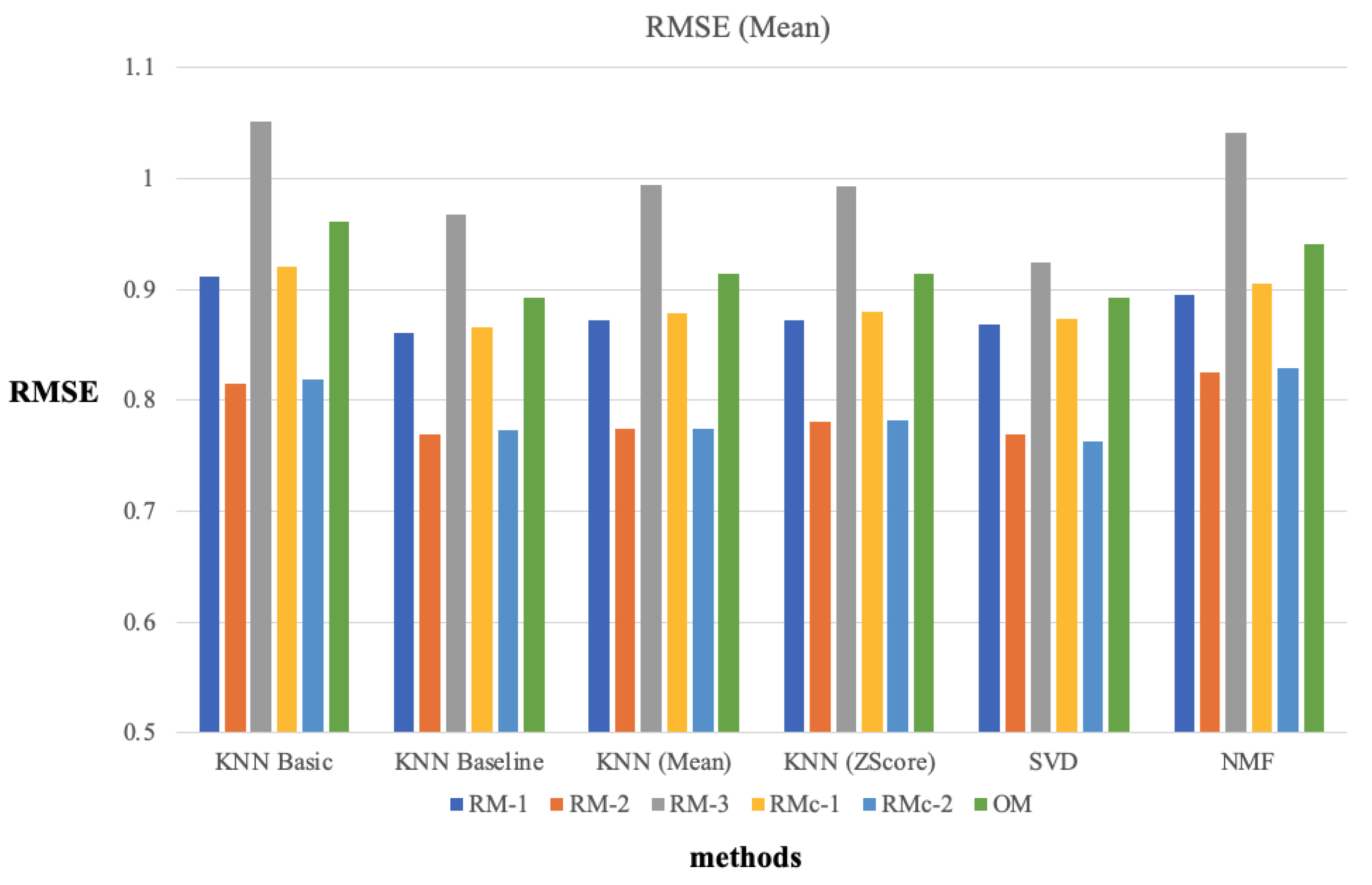
Similar results were demonstrated in the RMSE cases. It can be observed from Table 6 that RM-1 and RM-2 yielded higher accuracy when applying CF compared to the OM. There was no significant difference between RMc-1 and RMc-2, but the overall results of RM-1 and RM-2 were more accurate, respectively. Thus, the prediction results of applying the average ratio to the user genre preferences were more accurate than the prediction results obtained by concatenating each user ratio. Furthermore, it can be observed that the method using the PV filter yielded more accurate results than the OM.

Figure 9 and Figure 10 present the means in Table 5 and Table 6, respectively.

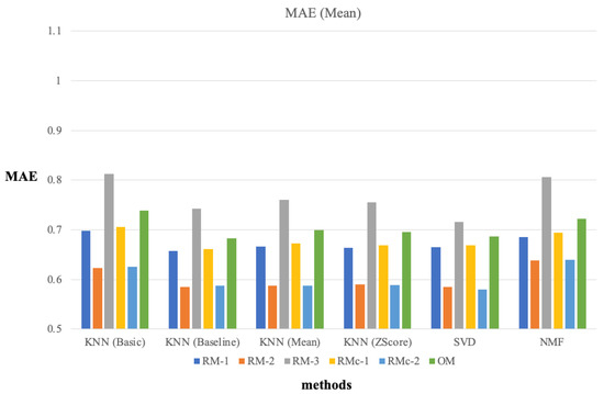
Figure 9. Average MAE of 10-fold cross-validation for each input matrix.

Figure 10. Average RMSE of 10-fold cross-validation for each input matrix..

The results of RM-2 and RMc-2, which selected items based on high average ratings, exhibited very high accuracy. Thus, the following hypothesis can be stated: “If the average of ratings constituting the matrix; that is, $r_{i,j}$ in the matrix, is high, the accuracy of the predictions is high”. To confirm this hypothesis, we computed the average of $r_{i,j}$ making up RM-1, RM-2, RM-3, and OM. Table 7 displays the averages and standard deviations of the ratings in each matrix.

Table 7. Averages and standard deviations of ratings in each matrix.

Method	Average	Standard Deviation
RM-1	3.5135	0.5470
RM-2	4.4453	0.3545
RM-3	3.3601	0.7041
OM	3.2921	0.8819

According to Table 7, the highest average was provided by RM-2. This is a reasonable result because the items were extracted from the OM in the order of high average ratings when regenerating RM-2. In comparison, the other three methodologies, namely RM-1, RM-3, and OM, did not extract the items in the order of average ratings, so it can be confirmed that these produced relatively lower averages than RM-2.

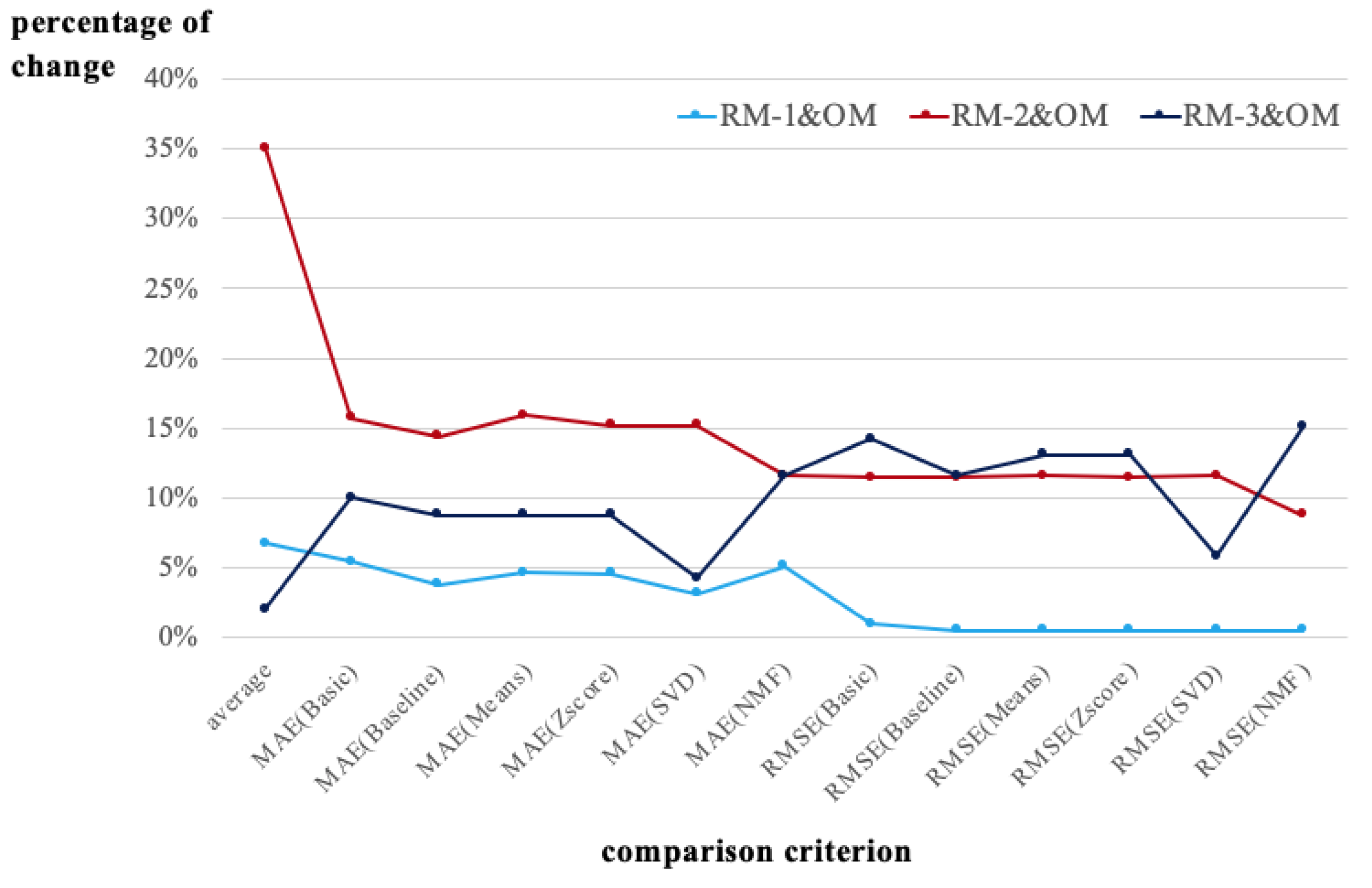
Based on the low MAE and RMSE, it can be observed that RM-1, which exhibited the best results apart from RM-2, had higher average ratings than the other two methods. In the case of OM, which had the next highest MAE and RMSE, the lowest average value was observed, and RM-3, which exhibited the worst accuracy as per Table 5 and Table 6, resulted in a higher average than the OM. Thus, a high average rating does not guarantee prediction accuracy. Furthermore, Figure 11 and Table 8 present the changes in the average, MAE, and RMSE of the different methodologies based on the OM in percentages. We calculated the change rates using Equation (11).

$$d_n=\frac{|val\left(R{M}_n\right)-val\left(OM\right)|}{val\left(OM\right)}\ast 100,$$

(11)

where $val\left(R{M}_n\right)$ and val(OM) indicate a value, such as the average, MAE, or RMSE for RM-n and the OM, respectively.

Figure 11. Change percentages for average, MAE, and RMSE of each method (OM-based).

Table 8. Change percentages for average, MAE, and RMSE of each method (OM-based).

Method	Average	Metric	KNN (Basic)	KNN (Baseline)	KNN (Means)	KNN (Zscore)	SVD	NMF
RM-1&OM	7%	MAE	5%	4%	5%	5%	3%	5%
RM-2&OM	35%		16%	14%	16%	15%	15%	12%
RM-3&OM	2%		10%	9%	9%	9%	4%	12%
RM-1&OM	7%	RMSE	1%	1%	1%	1%	1%	1%
RM-2&OM	35%		11%	11%	12%	11%	12%	9%
RM-3&OM	2%		14%	12%	13%	13%	6%	15%

In Figure 11, the x-axis and y-axis indicate the comparison criterion and change percentage, respectively. RM-1&OM represents the change of RM-1 based on the OM. For example, when the average rating of the OM was 3.29 and the average rating of RM-1 was 3.51, the average of RM-1&OM was $|3.29-3.51|/3.29$ * 100, which was approximately 6.7% (it could be rounded to 7%). If the average of RM-2 was 3.4, the average of RM-1&OM was $|3.29-3.4|/3.29$ * 100, which was approximately 3.3%. It means that the results derived from RM-2 is more close than RM-1 for the result derived from OM. The results were derived by applying this process to each methodology for the MAE and RMSE. RM-2&OM and RM-3&OM represent the changes of RM-2 and RM-3, respectively, based on the OM.

Comparing the change rates of the MAE and RMSE in Figure 11 and Table 8, it can be observed that, in all methodologies, there was a difference in the change rate for the average and that for the accuracy. The average change rate for RM-1&OM was approximately 7%. The change rate between the MAE and RMSE varied between approximately 1% and 5%. Moreover, the average change rate for RM-2&OM was approximately 35%, and the change rate of the MAE and RMSE ranged from approximately 9% to 16%. It can be observed from the comparison results that the change in the prediction results was insignificant compared to the change in the average values.

In the case of RM-3&OM, the change rate for the average was approximately 2%, whereas the change rate for the MAE and RMSE varied between approximately 9% and 16%. Accordingly, it can be confirmed that the change rate of the prediction accuracy was greater than that of the average, which means that the difference in the average rating has less of an effect on the accuracy.

4.3.2. Analysis of Sparsity

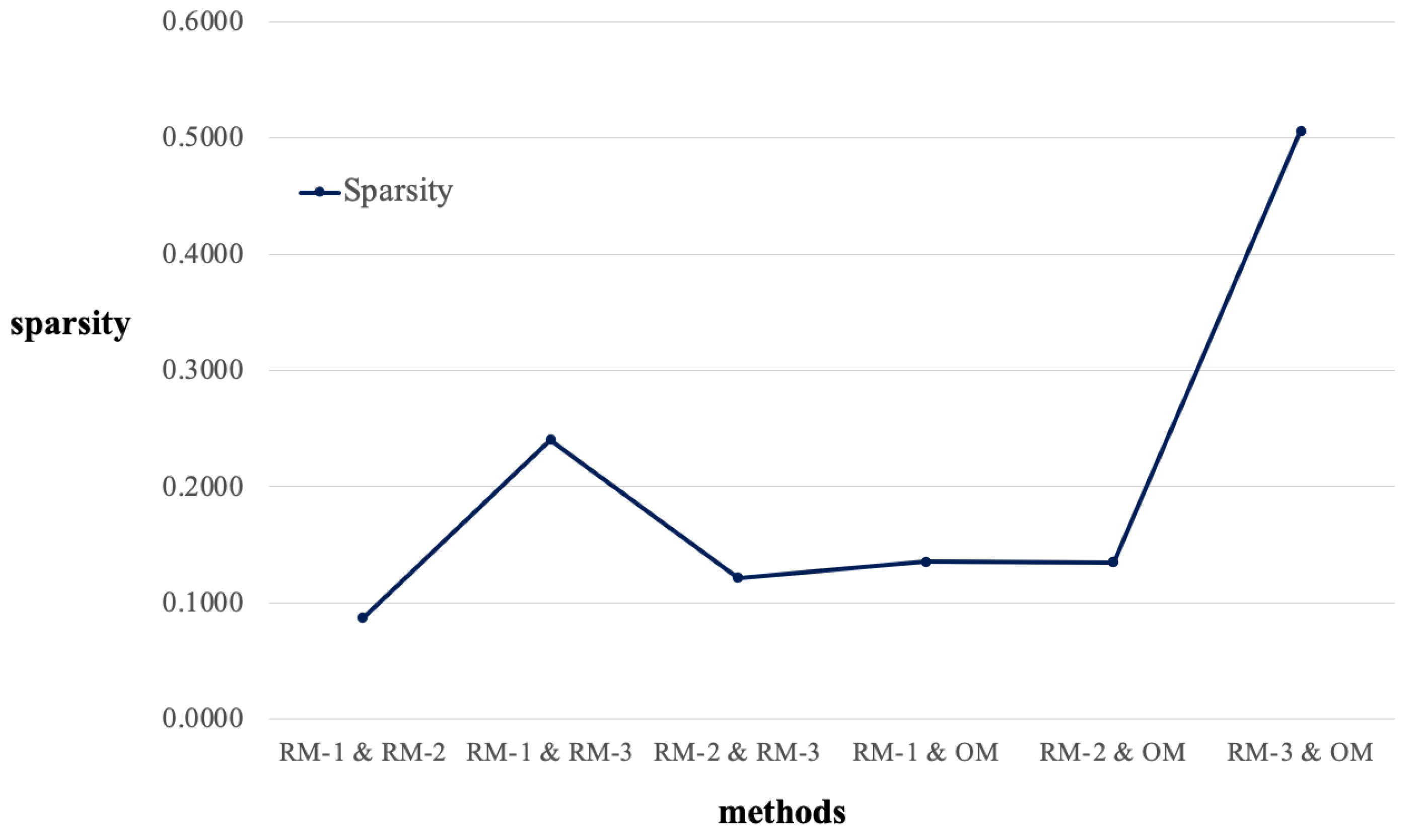
Our approach not only can improve the recommendation accuracy, but can also alleviate the data sparsity. Table 9 and Figure 12 present the data sparsity of the OM and RM. In Table 9, $usersize$ and $itemsize$ indicate the number of users and items in each matrix, respectively. Moreover, $\#ofratings$ denotes the number of ratings in each matrix and $sparsity$ indicates the amount of data sparsity in each matrix as the result of Equation (12).

$$SP=\frac{\#\mathrm{of}\mathrm{ratings}}{\mathrm{user}\mathrm{size}\ast \mathrm{item}\mathrm{size}}$$

(12)

Table 9. Data sparsity of OM and RM.

Method	Item Size	Sparsity
RM-1	1230	0.0685
RM-2	1223	0.0226
RM-3	4590	0.0070
OM	9125	0.0164

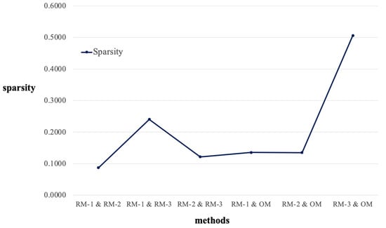
Figure 12. Data sparsity of OM and RM according to the various combinations of method.

It can be observed that the results for the sparsity of RM-1 and RM-2 were higher than those for the OM. This means that RM-1 and RM-2 had denser matrices than the OM; that is, when using two $RM$s, we can obtain more ratings and can apply CF based on the matrix with more ratings than the OM. Thus, through RM extraction, we can construct a denser matrix, which can alleviate the sparsity of the OM.

4.3.3. Analysis of Jaccard Similarity

We determined the similarities of the items composing each matrix to verify the differentiation of the results. For the verification, we used the Jaccard similarity, which can be derived according to Equation (13) [67].

$$J(X,Y)=\frac{|X\cap Y|}{|X\cup Y|},$$

(13)

where X and Y indicate sets. The result of the Jaccard similarity yields 1 when the two sets are the same and 0 when there is no common element. Therefore, the result of Equation (13) represents the ratio of the elements shared by two sets as a real number between 0 and 1.

For example, suppose that the sets of items in RM-1 and RM-2 are $I_1$ and $I_2$, respectively. If the elements of both sets are the same, the result of the Jaccard similarity is 1; if all elements are different, the result is 0.

Table 10 presents the results of the Jaccard similarity between the item sets of each matrix. It can be observed that the Jaccard similarity between RM-1 and RM-2, which had higher accuracy than the OM, was approximately 0.087. This means that the item lists of the two matrices shared approximately 9% of items. RM-1 and RM-2 exhibited superior performance over the OM, and Table 10 indicates that the ratio of items shared by the two matrices was actually smaller than the others. Therefore, it can be considered that the results obtained through the two matrices were not derived through matrices with similar contents.

Table 10. Jaccard similarity between item lists in each matrix.

Method	Jaccard Similarity
RM-1 & RM-2	0.0873
RM-1 & RM-3	0.2404
RM-2 & RM-3	0.1218
RM-1 & OM	0.1357
RM-2 & OM	0.1349
RM-3 & OM	0.5063

In conclusion, the high prediction accuracy and low sparsity of our approach are verified by comparisons with the OM results. We can check that the proposed method can improve the prediction accuracy of 16% and 15% for KNN and SVD, respectively. We can also find that a three times improvement in the sparsity based on RM-1&OM is obtained. Although our approach can improve existing methods by utilizing regenerated input, we cannot regenerate an input matrix in the absence of metadata and users’ reaction information in a domain. Therefore, we can consider that our experimental results can be derived for domains where users’ reaction data and metadata exist.

5. Conclusions

Recommendation systems operate based on the various user reactions to items. As such systems operate according to user responses, problems exist whereby recommendations are difficult to apply for new or less responsive items. Moreover, it is known that recommendations based on sparse datasets are less reliable.

Thus, we have proposed improving the sparseness and increasing the accuracy of the user–item matrix by using item features selected by users. Based on the content-based filtering (CBF) concept, the collaborative filtering (CF) input matrix was regenerated from the original user–item matrix by using item features, such as the category. That is, prior to applying the original user–item matrix to CF, we regenerated the matrix as the CF input.

We first extracted the category ratio of the selected item by users. Moreover, we proposed a method for regenerating the original user–item matrix based on the extracted ratio. We assumed that the regenerated matrix (RM) considered the user preferences compared to the original matrix (OM) and applied it to CF.

Our contributions can be divided into academic and industrial sides. Based on the academic contributions, we can solve our research question. The academic contributions are summarized as follows:

• We have proposed a novel approach that can regenerate the input from the OM for CF by constructing user PVs based on category selection rates and filtering the OM through user PVs.
• The accuracy was verified by applying the regenerated input matrices to a total of six CF approaches. The prediction accuracy of the proposed method was verified through comparative experiments using the OM as input.
• We have demonstrated that the results obtained by our approach are more precise than those of conventional CF approaches.
• The low sparsity and high prediction accuracy of the proposed method were verified by comparisons with the OM results. (Improvements of approximately 16% based on KNN (MAE) and 15% based on SVD (MAE), and a three times improvement in the sparsity based on RM-1&OM were obtained.)

The recommender systems based on collaborative filtering approaches are currently addressed in various web services, such as Amazon and Netflix [1,2,5]. These approaches utilize the user–item rating matrix as input to generate recommendation results. Because of this reason, if we can construct the same shape of the input matrix, then we can utilize the constructed matrix as the input of the collaborative filtering approaches.

In our approach, we have reconstructed the input as the same structure by utilizing the original input matrix. It means that if the original matrix has users as a row and items as a column, the reconstructed matrix also has the same row and column. Because of this reason, we can easily apply our approach to the conventional collaborative filtering approaches. The industrial contributions of our approach are summarized as follows:

• In the case of e-commerce or media content recommendation systems, most of them suffer from sparsity problems for input data. The matrix reconstruction scheme proposed in this paper can alleviate the sparsity problems for the real inputs.
• Furthermore, based on the input matrix with reduced sparsity, we can derive a higher prediction accuracy than the existing input for the aspect of the average ratings.
• Through our approach, it is possible to provide more reliable recommendation results to online service users with less input.
• In addition, online service providers can build more reliable recommender systems based on less data.

We regenerated the matrix using the number of selections and average ratings of the items. The results were compared using the random-based RM and OM as inputs for the CF. We tested our approach using the MAE and RMSE. Moreover, we confirmed that the RM produced higher recommendation accuracy than the results obtained through the OM.

The sparsity of each matrix was calculated and the proposed matrix was verified to be denser than the OM. The differences in the items contained in the RM were demonstrated by calculating the Jaccard similarity of the set of items in each matrix. On this basis, we verified the differentiation of the RM derived from each methodology, and, finally, a method for constructing a denser input matrix, as well as a method for deriving high accuracy were presented.

We have proposed and simulated our approach based on the MovieLens dataset, however, we can apply the regenerated method to other domains such as music, books, and e-commerce items. Namely, if the domain has category information and users’ reaction to the items in the domain, we can regenerate the input matrix since our approach has utilized the feature for the item. Thus, there exist the possibility to apply our approach to various types of domains that have item features such as category information.

In future work, we will apply this approach to more diverse databases with various item features to analyze the results. Furthermore, we will apply the user PVs obtained through the item features to cross-domain recommender systems to verify the usability.

In addition, as deep learning-based recommender system studies progress, it the embedding approaches has been proposed in various ways using autoencoder or item2vec. We have introduced the data preprocessing process based on item features that can be used in terms of deep learning recommendation model. In other words, we have suggested the method of regenerating the input matrix to a more dense form by using the item features. The proposed method can be used as an input to various deep learning recommendation models.

References

- Sarwar, B.M.; Karypis, G.; Konstan, J.A.; Riedl, J. Item-based Collaborative Filtering Recommendation Algorithms. In Proceedings of the 10th International World Wide Web Conference (WWW ’01), Hong Kong, China, 1–5 May 2001; pp. 285–295. [Google Scholar]
- Herlocker, J.L.; Konstan, J.; Borchers, A.; Riedl, J. An Algorithm Framework for Peforming Collaborative Filtering. In Proceedings of the 22nd Annual International ACM SIGIR Conference on Research and Development in Information Retrieval (SIGIR ’99), Berkeley, CA, USA, 15–19 August 1999; pp. 230–237. [Google Scholar]
- Tkalcic, M.; Odic, A.; Kosir, A.; Tasic, J.F. Affective Labeling in a Content-Based Recommender System for Images. IEEE Trans. Multimedia 2013, 15, 391–400. [Google Scholar] [CrossRef]
- Ricci, F.; Rokach, L.; Shapira, B.; Kantor, P.B. Recommender Systems Handbook; Springer: Berlin/Heidelberg, Germany, 2010. [Google Scholar]
- Koren, Y.; Bell, R.M.; Volinsky, C. Matrix Factorization Techniques for Recommender Systems. IEEE Comput. 2009, 42, 30–37. [Google Scholar] [CrossRef]
- de Campos, L.; Fernández-Luna, J.; Huete, J.; Rueda-Morales, M. Combining content-based and collaborative recommendations: A hybrid approach based on Bayesian networks. Int. J. Approx. Reason. 2010, 51, 785–799. [Google Scholar] [CrossRef]
- Çano, Erion and Morisio, Maurizio Hybrid Recommender Systems: A Systematic Literature Review. Intell. Data Anal. 2017, 21, 1487–1524. [CrossRef]
- He, X.; Liao, L.; Zhang, H.; Nie, L.; Hu, X. Neural Collaborative Filtering. In Proceedings of the 26th International Conference on World Wide Web (WWW 17), Perth, Australia, 3–7 April 2017; pp. 173–182. [Google Scholar]
- Liang, D.; Krishnan, R.G. Variational Autoencoders for Collaborative Filtering. In Proceedings of the 2018 World Wide Web Conference (WWW 18), Lyon, France, 23–27 April 2018; pp. 689–698. [Google Scholar]
- Duong, T.N.; Vuong, T.A.; Nguyen, D.M.; Dang, Q.H. Utilizing an Autoencoder-Generated Item Representation in Hybrid Recommendation System. IEEE Access 2020, 8, 75094–75104. [Google Scholar] [CrossRef]
- Barkan, O.; Koenigstein, N. Item2Vec: Neural Item Embedding for Collaborative Filtering. CoRR 2016, abs/1603.04259. Available online: https://arxiv.org/abs/1603.04259 (accessed on 20 February 2017).
- Chen, C.; Wang, C.; Tsai, M.; Yang, Y. Collaborative Similarity Embedding for Recommender Systems. In Proceedings of the World Wide Web Conference (WWW 2019), Thessaloniki, Greece, 14–17 October 2019; pp. 2637–2643. [Google Scholar]
- Zhao, X.; Liu, H.; Liu, H.; Tang, J.; Guo, W.; Shi, J.; Wang, S.; Gao, H.; Long, B. AutoDim: Field-aware Embedding Dimension Searchin Recommender Systems. In Proceedings of the WWW ’21: The Web Conference 2021, Virtual, 12–23 April 2021; pp. 3015–3022. [Google Scholar]
- Zhu, Z.; Wang, J.; Caverlee, J. Improving Top-K Recommendation via JointCollaborative Autoencoders. In Proceedings of the World Wide Web Conference (WWW 2019), San Francisco, CA, USA, 13–17 May 2019; pp. 3482–3483. [Google Scholar]
- Khawar, F.; Poon, L.K.M.; Zhang, N.L. Learning the Structure of Auto-Encoding Recommenders. In Proceedings of the WWW ’20: The Web Conference 2020, Taipei, Taiwan, 20–24 April 2020; pp. 519–529. [Google Scholar]
- Xie, Z.; Liu, C.; Zhang, Y.; Lu, H.; Wang, D.; Ding, Y. Adversarial and Contrastive Variational Autoencoder for Sequential Recommendation. In Proceedings of the WWW ’21: The Web Conference 2021, Virtual, 12–23 April 2021; pp. 449–459. [Google Scholar]
- Rendle, S.; Krichene, W.; Zhang, L.; Anderson, J.R. Neural Collaborative Filtering vs. Matrix Factorization Revisited. In Proceedings of the RecSys 2020: Fourteenth ACM Conference on Recommender Systems (RecSys ’20), Virtual, 22–26 September 2020; pp. 240–248. [Google Scholar]
- Schein, A.I.; Popescul, A.; Ungar, L.H.; Pennock, D.M. Methods and metrics for cold-start recommendations. In Proceedings of the 25th Annual International ACM SIGIR Conference on Research and Development in Information Retrieval (SIGIR ’02), Tampere, Finland, 11–15 August 2002; pp. 253–260. [Google Scholar]
- Ishikawa, M.; Géczy, P.; Izumi, N.; Morita, T.; Yamaguchi, T. Information Diffusion Approach to Cold-Start Problem. In Proceedings of the 2007 IEEE/WIC/ACM International Conference on Web Intelligence and International Conference on Intelligent Agent Technology–Workshops (WI-IAT ’07), Silicon Valley, CA, USA, 5–12 November 2007; pp. 129–132. [Google Scholar]
- Said, A.; Jain, B.; Narr, S.; Plumbaum, T. Users and Noise: The Magic Barrier of Recommender Systems. In Proceedings of the 20th Conference on User Modelling, Adaptation, and Personalization, Montreal, QC, Canada, 16–20 July 2012; Volume 7379. [Google Scholar]
- Bellogín, A.; Said, A.; de Vries, A. The Magic Barrier of Recommender Systems–No Magic, Just Ratings. In Proceedings of the 22nd International Conference on User Modelling, Adaptation, and Personalization, Aalborg, Denmark, 7–11 July 2014; pp. 25–36. [Google Scholar]
- Sarwar, B.M.; Karypis, G.; Konstan, J.A.; Riedl, J. Analysis of recommendation algorithms for e-commerce. In Proceedings of the 2nd ACM Conference on Electronic Commerce (EC ’00), Minneapolis, MN, USA, 17–20 October 2000; pp. 158–167. [Google Scholar]
- Bell, R.M.; Koren, Y. Lessons from the Netflix prize challenge. Sigkdd Explor. 2007, 9, 75–79. [Google Scholar] [CrossRef]
- Levy, O.; Goldberg, Y. Neural Word Embedding as Implicit Matrix Factorization. In Proceedings of the Advances in Neural Information Processing Systems 27: Annual Conference on Neural Information Processing Systems 2014, Montreal, QC, Canada, 8–13 December 2014; pp. 2177–2185. [Google Scholar]
- Wei, K.; Huang, J.; Fu, S. A Survey of E-Commerce Recommender Systems. In Proceedings of the 2007 International Conference on Service Systems and Service Management, Chengdu, China, 9–11 June 2007; pp. 1–5. [Google Scholar]
- Bobadilla, J.; Ortega, F.; Hernando, A.; Gutiérrez, A. Recommender systems survey. Knowl.-Based Syst. 2013, 46, 109–132. [Google Scholar] [CrossRef]
- Ronen, R.; Koenigstein, N.; Ziklik, E.; Nice, N. Selecting Content-Based Features for Collaborative Filtering Recommenders. In Proceedings of the 7th ACM Conference on Recommender Systems (RecSys ’13), Hong Kong, China, 12–16 October 2013; pp. 407–410. [Google Scholar]
- Choi, S.M.; Ko, S.K.; Han, Y.S. A movie recommendation algorithm based on genre correlations. Expert Syst. Appl. 2012, 39, 8079–8085. [Google Scholar] [CrossRef]
- Pirasteh, P.; Jung, J.J.; Hwang, D. Item-Based Collaborative Filtering with Attribute Correlation: A Case Study on Movie Recommendation. In Proceedings of the Intelligent Information and Database Systems–6th Asian Conference (ACIIDS ’14), Bangkok, Thailand, 7–9 April 2014; pp. 245–252. [Google Scholar]
- Zhang, J.; Peng, Q.; Sun, S.; Liu, C. Collaborative filtering recommendation algorithm based on user preference derived from item domain features. Phys. Stat. Mech. Its Appl. 2014, 396, 66–76. [Google Scholar] [CrossRef]
- Christensen, I.; Schiaffino, S. A Hybrid Approach for Group Profiling in Recommender Systems. J. Univers. Comput. Sci. 2014, 20, 507–533. [Google Scholar]
- Lekakos, G.; Giaglis, G. A hybrid approach for improving predictive accuracy of collaborative filtering algorithms. User Model. User-Adapt. Interact. 2007, 17, 5–40. [Google Scholar] [CrossRef]
- Çano, E.; Morisio, M. Hybrid Recommender Systems: A Systematic Literature Review. CoRR 2019, abs/1901.03888. Available online: https://arxiv.org/abs/1901.03888 (accessed on 12 January 2019).
- Rojsattarat, E.; Soonthornphisaj, N. Hybrid Recommendation: Combining Content-Based Prediction and Collaborative Filtering. In Proceedings of the Intelligent Data Engineering and Automated Learning; Springer: Berlin/Heidelberg, Germany, 2003; pp. 337–344. [Google Scholar]
- Lang, K. NewsWeeder: Learning to Filter Netnews. In Proceedings of the Twelfth International Conference on Machine Learning, Tahoe City, CA, USA, 9–12 July 1995; pp. 331–339. [Google Scholar]
- Krulwich, B. Learning user interests across heterogeneous document databases. In Proceedings of the 1995 AAAI Spring Symposium Series, Palo Alto, CA, USA, 27–29 March 1995; pp. 106–110. [Google Scholar]
- Chughtai, M.W.; Selamat, A.; Ghani, I.; Jung, J. E-Learning Recommender Systems Based on Goal-Based Hybrid Filtering. Int. J. Distrib. Sens. Netw. 2014, 2014. [Google Scholar] [CrossRef]
- Burke, R. Hybrid Recommender Systems: Survey and Experiments. User Model.-User-Adapt. Interact. 2002, 12, 331–370. [Google Scholar] [CrossRef]
- Lika, B.; Kolomvatsos, K.; Hadjiefthymiades, S. Facing the cold start problem in recommender systems. Expert Syst. Appl. 2014, 41, 2065–2073. [Google Scholar] [CrossRef]
- Carrer-Neto, W.; Hernández-Alcaraz, M.L.; Valencia-García, R.; García-Sánchez, F. Social knowledge-based recommender system. Application to the movies domain. Expert Syst. Appl. 2012, 39, 10990–11000. [Google Scholar] [CrossRef]
- Ghazanfar, M.A.; Prügel-Bennett, A. The Advantage of Careful Imputation Sources in Sparse Data-Environment of Recommender Systems: Generating Improved SVD-based Recommendations. Informatica (Slovenia) 2013, 37, 61–92. [Google Scholar]
- Choi, S.M.; Han, Y.S. Identifying representative ratings for a new item in recommendation system. In Proceedings of the 7th International Conferenece on Ubiquitous Information Management and Communication (ICUIMC ’13), Kota Kinabalu, Malaysia, 17–19 January 2013; p. 64. [Google Scholar]
- Gantner, Z.; Drumond, L.; Freudenthaler, C.; Rendle, S.; Schmidt-Thieme, L. Learning Attribute-to-Feature Mappings for Cold-Start Recommendations. In Proceedings of the 10th IEEE International Conference on Data Mining (ICDM ’10), Sydney, Australia, 13–17 December 2010; pp. 176–185. [Google Scholar]
- Sun, D.; Luo, Z.; Zhang, F. A novel approach for collaborative filtering to alleviate the new item cold-start problem. In Proceedings of the 11th International Symposium on Communications and Information Technologies (ISCIT ’11), Hangzhou, China, 12–14 October 2011; pp. 402–406. [Google Scholar]
- Volkovs, M.; Yu, G.W.; Poutanen, T. Content-based Neighbor Models for Cold Start in Recommender Systems. In Proceedings of the Recommender Systems Challenge 2017 (RecSys Challenge ’17), Como, Italy, 27–31 August 2017; pp. 7:1–7:6. [Google Scholar] [CrossRef]
- Deng, Y.; Wu, Z.; Tang, C.; Si, H.; Xiong, H.; Chen, Z. A Hybrid Movie Recommender Based on Ontology and Neural Networks. In Proceedings of the 2010 IEEE/ACM International Conference on Green Computing and Communications International Conference on Cyber, Physical and Social Computing, Washington, DC, USA, 18–20 December 2010; pp. 846–851. [Google Scholar]
- Wen, H.; Fang, L.; Guan, L. A hybrid approach for personalized recommendation of news on the Web. Expert Syst. Appl. Int. J. 2012, 39, 5806–5814. [Google Scholar] [CrossRef]
- Meel, P.; Bano, F.; Goswami, A.; Gupta, S. Movie Recommendation Using Content-Based and Collaborative Filtering. In Proceedings of the International Conference on Innovative Computing and Communications (ICICC ’21); Springer: Singapore, 2021; pp. 301–316. [Google Scholar]
- Chen, S.; Huang, L.; Lei, Z.; Wang, S. Research on personalized recommendation hybrid algorithm for interactive experience equipment. Comput. Intell. 2020, 36, 1348–1373. [Google Scholar] [CrossRef]
- Mehrabani, M.M.; Mohayeji, H.; Moeini, A. A Hybrid Approach to Enhance Pure Collaborative Filtering Based on Content Feature Relationship. Available online: https://arxiv.org/abs/2005.08148 (accessed on 17 May 2020).
- Zhao, W.; Tian, H.; Wu, Y.; Cui, Z.; Feng, T. A New Item-Based Collaborative Filtering Algorithm to Improve the Accuracy of Prediction in Sparse Data. Int. J. Comput. Intell. Syst. 2022, 15, 1–15. [Google Scholar] [CrossRef]
- Althbiti, A.; Alshamrani, R.; Alghamdi, T.; Lee, S.; Ma, X. Addressing Data Sparsity in Collaborative Filtering Based Recommender Systems Using Clustering and Artificial Neural Network. In Proceedings of the 2021 IEEE 11th Annual Computing and Communication Workshop and Conference (CCWC), Virtual, 27–30 January 2021; pp. 0218–0227. [Google Scholar] [CrossRef]
- Jiang, B.; Yang, J.; Qin, Y.; Wang, T.; Wang, M.; Pan, W. A Service Recommendation Algorithm Based on Knowledge Graph and Collaborative Filtering. IEEE Access 2021, 9, 50880–50892. [Google Scholar] [CrossRef]
- Ahmadian, S.; Joorabloo, N.; Jalili, M.; Ahmadian, M. Alleviating data sparsity problem in time-aware recommender systems using a reliable rating profile enrichment approach. Expert Syst. Appl. 2022, 187, 115849. [Google Scholar] [CrossRef]
- Chen, H.; Qian, F.; Chen, J.; Zhao, S.; Zhang, Y. Attribute-based Neural Collaborative Filtering. Expert Syst. Appl. 2021, 185, 115539. [Google Scholar] [CrossRef]
- Ajaegbu, C. An optimized item-based collaborative filtering algorithm. J. Ambient. Intell. Humaniz. Comput. 2021, 12, 10629–10636. [Google Scholar] [CrossRef]
- khaledian, N.; Mardukhi, F. CFMT: A collaborative filtering approach based on the nonnegative matrix factorization technique and trust relationships. J. Ambient. Intell. Humaniz. Comput. 2022, 13, 2667–2683. [Google Scholar] [CrossRef]
- Zhou, Q.; Zhuang, W.; Ren, H.; Chen, Y.; Yu, B.; Lou, J.; Wang, Y. Hybrid Collaborative Filtering Model for Consumer Dynamic Service Recommendation Based on Mobile Cloud Information System. Inf. Process. Manag. 2022, 59, 102871. [Google Scholar] [CrossRef]
- Liu, H.; Guo, L.; Li, P.; Zhao, P.; Wu, X. Collaborative filtering with a deep adversarial and attention network for cross-domain recommendation. Inf. Sci. 2021, 565, 370–389. [Google Scholar] [CrossRef]
- Lin, Z.; Tian, C.; Hou, Y.; Zhao, W.X. Improving Graph Collaborative Filtering with Neighborhood-Enriched Contrastive Learning. In Proceedings of the ACM Web Conference 2022 (WWW ’22), Athens, Greece, 26–29 June 2022; Association for Computing Machinery: New York, NY, USA, 2022; pp. 2320–2329. [Google Scholar]
- Aljunid, M.F.; Huchaiah, M.D. IntegrateCF: Integrating explicit and implicit feedback based on deep learning collaborative filtering algorithm. Expert Syst. Appl. 2022, 207, 117933. [Google Scholar] [CrossRef]
- Surprise. k-NN Inspired Algorithms. Available online: https://surprise.readthedocs.io/en/stable/knn_inspired.html (accessed on 25 September 2017).
- Bulmer, M.G. Principle of Statistics; Dover Publications: New York, NY, USA, 1979. [Google Scholar]
- Surprise. Matrix Factorization-Based Algorithms. Available online: https://surprise.readthedocs.io/en/stable/matrix_factorization.html (accessed on 17 March 2017).
- Choi, S.M.; Cha, J.W.; Han, Y.S. Identifying representative reviewers in internet social media. In Proceedings of the Second International Conference on Computational Collective Intelligence: Technologies and Applications–Volume Part II (ICCCI ’10), Kaohsiung, Taiwan, 10–12 November 2010; pp. 22–30. [Google Scholar]
- Choi, S.M.; Cha, J.W.; Kim, L.; Han, Y.S. Reliability of Representative Reviewers on the Web. In Proceedings of the International Conference on Information Science and Applications–ICISA, Jeju Island, Republic of Korea, 26–29 April 2011; pp. 1–5. [Google Scholar]
- Jaccard, P. The distribution of the flora in the alpine zone. New Phytol. 1912, 11, 37–50. [Google Scholar] [CrossRef]
Disclaimer/Publisher’s Note: The statements, opinions and data contained in all publications are solely those of the individual author(s) and contributor(s) and not of MDPI and/or the editor(s). MDPI and/or the editor(s) disclaim responsibility for any injury to people or property resulting from any ideas, methods, instructions or products referred to in the content. |
© 2023 by the authors. Licensee MDPI, Basel, Switzerland. This article is an open access article distributed under the terms and conditions of the Creative Commons Attribution (CC BY) license (https://creativecommons.org/licenses/by/4.0/).