Two Families of Continuous Probability Distributions Generated by the Discrete Lindley Distribution

Abstract

In this paper, we construct two new families of distributions generated by the discrete Lindley distribution. Some mathematical properties of the new families are derived. Some special distributions from these families can be constructed by choosing some baseline distributions, such as exponential, Pareto and standard logistic distributions. We study in detail the properties of the two models resulting from the exponential baseline, among others. These two models have different shape characteristics. The model parameters are estimated by maximum likelihood, and related algorithms are proposed for the computation of the estimates. The existence of the maximum-likelihood estimators is discussed. Two applications prove its usefulness in real data fitting.

1. Introduction

Compound discrete distributions serve as probabilistic models in various areas of applications, for instance, in ecology, genetics and physics. See, for example, [1]. Distributions obtained by compounding a parent distribution with a discrete distribution are very common in statistics and in many applied areas. Suppose we have a system consisting of N components, the lifetime of each of which is a random variable. Let X be the maximum lifetime of the components. Clearly, X has a compound distribution arising out of a random number N of components; i.e., $X=max\{Z_1,\dots ,Z_N\}$. On the other hand, in case of a system consisting of N components whose energy consumption is a random variable, and assuming that Z is the component whose energy consumption is minimal, we obtain the compound distribution of $Y=min\{Z_1,\dots ,Z_N\}.$ The compounding principle is applied in the many different areas: insurance [2], ruin problems [3], compound risk models and their actuarial applications [4,5]. The development of the theory of compounding distribution is skipped here, because it has been covered in detail in [6].

The random variable N is often determined by economy, customer demand, etc. There is a practical reason why N might be considered as a random variable. A failure can occur due to initial defects being present in the system. A discrete version of this distribution has been studied in [7], having its applications in count data related to insurance.

We will say that random variable X possesses the discrete Lindley distribution introduced by [7] if its probability mass function is given by

$$P(X=x)=\frac{{\lambda }^x}{1-log\lambda }[\lambda log\lambda +(1-\lambda )(1-log{\lambda }^{x+1})],$$

where $x=0,1,\dots$ and $0<\lambda <1.$ The probability generating function (PGF) (see Equation (4) in [7]) is given by the typo error. The corrected version is defined by

$$\Phi \left(s\right)=\frac{(\lambda -1)(\lambda s-1)-(1-2\lambda +{\lambda }^{2}s)log\left(\lambda \right)}{{(1-\lambda s)}^2(1-log\left(\lambda \right))},s<1/\lambda ,0<\lambda <1.$$

(1)

In this manuscript, we consider the previously discrete Lindley distribution for the random variable $N.$ Why do we assume a discrete Lindley distribution? For example, using a Poisson distribution has an important assumption: equidispersion of data. The assumption of equidispersion is not valid in real cases. Some alternative distributions to the model of overdispersed data are available—binomial negative, generalized Poisson or zero inflated Poisson. However, judging by the number of parameters used, these alternatives are more complex than the Poisson distribution. That is why we are introducing a continuous Lindley distribution with one parameter, which is similar to the Poisson distribution. The application of the Lindley distribution in modeling the number of claim data is less suitable because the number of claims data is a discrete number, as opposed to the Lindley distribution’s continuous nature. That is why we are introducing a new discrete Lindley distribution, created through discretisation of a continuous Lindley distribution with one parameter.

Assuming that M is the zero truncated version of N with PGF (1), we will construct two new families of distributions: the discrete Lindley-generated families of distributions of the first and second kinds.

The paper is organized as follows. In Section 1, we construct two discrete Lindley generated families. Section 2 is devoted to shape characteristics. In Section 3 we derive some mathematical properties of the families. Estimation issues are investigated in Section 4 and Section 5. The simulation study is presented in Section 6. Two applications to real data are addressed in Section 7. The paper is finalized with concluding remarks.

2. Construction of the Families of Distributions

There are various methods for getting the discrete Lindley distribution. For example, in [8], the authors considered a method of infinite series for constructing the discrete Lindley distribution. On the other hand, in [9], the discrete Lindley distribution was built using the survival function method. In this manuscript, we employ the so-called max-min procedure. This construction is widely used in practice. For a comprehensive literature review, we refer the reader to [10] and references therein.

In this section, we introduce two new families of distributions as follows. Let ${\left\{Z_i\right\}}_{i\ge 1}$ be a sequence of independent and identically distributed (iid) random variables with baseline cumulative distribution function (CDF) $F\left(x\right)=F(x;\psi )$, where $x\in \mathbb{R}$ and $\psi$ is the parameter vector. Suppose that N is a discrete random variable with the PGF $\Phi \left(s\right)$ and let M have the zero-truncated distribution of the random variable N obtained by removing zero from N. Then, the probability mass function (pmf) of M is given by

$$P(M=m)=\frac{P(N=m)}{1-\Phi \left(0\right)},m\in \{1,2,\cdots \}.$$

(2)

In order to prove that ${\displaystyle \sum _{m=1}^{+\infty }}P(M=m)=1$, let us recall that $P(N=m)=\frac{{\Phi }^m\left(0\right)}{m!}$. After some algebra, we find

$$P(N=m)={\lambda }^m\frac{\lambda -1+log\lambda -2\lambda log\lambda }{log\lambda -1}+\frac{m{\lambda }^m(1-\lambda )log\lambda }{log\lambda -1}.$$

Using serial representations ${\sum }_{m=1}^{+\infty }{\lambda }^m=\frac{\lambda }{1-\lambda }$ and ${\sum }_{m=1}^{+\infty }m{\lambda }^m=\frac{\lambda }{{(1-\lambda )}^2}$, one can calculate

$$\sum _{m=1}^{+\infty }P(N=m)=\frac{\lambda (1-2log\lambda )}{1-log\lambda }.$$

(3)

Equation (3) coincides with $1-\Phi \left(0\right).$ This completes the proof that ${\displaystyle \sum _{m=1}^{+\infty }}P(M=m)=1.$

First, we introduce the family of distributions based on the maximum of random variables. We define the random variable $X=max{\left\{Z_i\right\}}_{i=1}^M$. Then, the CDF and probability density function (PDF) of X are given by

$$G_X\left(x\right)=\frac{\Phi \left[F\right(x\left)\right]}{1-\Phi \left(0\right)},x\in \mathbb{R}$$

and

$$g_X\left(x\right)=\frac{f\left(x\right){\Phi }^{\prime }\left[F\left(x\right)\right]}{1-\Phi \left(0\right)},x\in \mathbb{R},$$

respectively.

Further, if we suppose that the random variable N has the PGF given by (1), the CDF and PDF of X for $x\in \mathbb{R},\lambda \in (0,1)$ are given by

$$G_1\left(x\right)=G_1(x;\theta ,\lambda )=\frac{F\left(x\right)[1-\lambda +(3\lambda -2)log(\lambda )-\lambda (1-\lambda +(2\lambda -1)log\left(\lambda \right)\left)F\right(x\left)\right]}{(1-2log\left(\lambda \right)){[1-\lambda F\left(x\right)]}^2},$$

(4)

and

$$g_1\left(x\right)=\frac{f\left(x\right)[1-\lambda +(3\lambda -2)log(\lambda )-\lambda (1-\lambda +\lambda log\left(\lambda \right)\left)F\right(x\left)\right]}{(1-2log\left(\lambda \right)){[1-\lambda F\left(x\right)]}^3},$$

(5)

respectively. We say that the family of distributions defined by (4) and (5) is the discrete Lindley generated family of the first kind (“LiG1” for short). A random variable X having PDF (5) is denoted by $X\sim$LiF1$(\lambda ,\psi )$.

The hazard rate function (HRF) of X can be expressed as

$${\tau }_1\left(x\right)=\frac{h_F\left(x\right)[1-\lambda +(3\lambda -2)log\left(\lambda \right)-\lambda (1-\lambda +\lambda log\left(\lambda \right))F\left(x\right)]}{[1-\lambda F(x\left)\right][1-2log(\lambda )-\lambda (1-log\left(\lambda \right)\left)F\right(x\left)\right]},x\in \mathbb{R},\lambda \in (0,1).$$

(6)

Let us study the identifiable property of the distribution given by (4) under the exponential baseline distribution $F(x;\theta )=1-e^{-\theta x}$. We will get the discrete Lindley exponential distribution of the first kind. We will designate this distribution LiE1.

Theorem 1. 

The LiE1 distribution is identifiable with respect to the parameters λ and $\theta .$

Proof. 

Let us suppose that

$$G_1(x;{\theta }_1,{\lambda }_1)=G_1(x;{\theta }_2,{\lambda }_2)$$

(7)

for all $x>0$ and when $F\left(x\right)$ is the CDF of exponential distribution. If we let $x\to \infty$ into both sides of (7) and after some algebra, it can be concluded that ${\lambda }_1={\lambda }_2$. Now it is not hard to verify that ${\theta }_1={\theta }_2.$ Hence the proof of the theorem.    □

Second, in [6], it was demonstrated that the random variable $Y=min{\left\{Z_i\right\}}_{i=1}^M$ has CDF and PDF given by

$$G_Y\left(y\right)=\frac{1-\Phi [1-F(y\left)\right]}{1-\Phi \left(0\right)},y\in \mathbb{R},$$

(8)

and

$$g_Y\left(y\right)=\frac{f\left(y\right){\Phi }^{\prime }[1-F\left(y\right)]}{1-\Phi \left(0\right)},y\in \mathbb{R},$$

(9)

respectively.

Now, inserting (1) in Equation (8), the CDF of the random variable Y becomes

$$G_2\left(x\right)=G_2(x;\theta ,\lambda )=\frac{F\left(x\right)[1-2log\left(\lambda \right)-\lambda (1-log\left(\lambda \right))\overline{F}\left(x\right)]}{(1-2log\left(\lambda \right)){[1-\lambda \overline{F}\left(x\right)]}^2},x\in \mathbb{R},\lambda \in (0,1),$$

(10)

where $\overline{F}\left(x\right)=1-F\left(x\right)$ is the survival function of the random variable $Z_1$.

In a similar manner, by replacing (1) in the Equation (9), the PDF of Y reduces to

$$g_2\left(x\right)=\frac{f\left(x\right)[1-\lambda +(3\lambda -2)log\left(\lambda \right)-\lambda (1-\lambda +\lambda log\left(\lambda \right))\overline{F}\left(x\right)]}{(1-2log\left(\lambda \right)){[1-\lambda \overline{F}\left(x\right)]}^3},x\in \mathbb{R},\lambda \in (0,1).$$

(11)

The random variable Y having the PDF (11) is called the discrete Lindley generated family of the second kind, $Y\sim$LiF2$(\lambda ,\psi )$.

From Equations (10) and (11), the HRF of Y follows as

$${\tau }_2\left(x\right)=\frac{h_F\left(x\right)[1-\lambda +(3\lambda -2)log\left(\lambda \right)-\lambda (1-\lambda +\lambda log\left(\lambda \right))\overline{F}\left(x\right)]}{[1-\lambda \overline{F}\left(x\right)][1-\lambda +(3\lambda -2)log\left(\lambda \right)-\lambda (1-\lambda +(2\lambda -1)log\left(\lambda \right))\overline{F}\left(x\right)]},x\in \mathbb{R},\lambda \in (0,1),$$

(12)

where ${\tau }_F\left(x\right)=f\left(x\right)/\overline{F}\left(x\right)$ is the HRF of the random variable $Z_i$.

There are at least four motivations for having two families of distributions: Reliability: From the stochastic representations X and Y, we note that the two families can arise in parallel and series systems with identical components, which appear in many industrial applications and biological organisms. The first-activation scheme: If we assume that an individual is susceptible to a cancer type, then we can call the number of carcinogenic cells that survived the initial treatment M, and $Z_i$ is the time needed for the $i-$th carcinogenic cell to metastasise into a detectable tumour, for $i\ge 1$. If we assume that ${\left\{Z_i\right\}}_{i\ge 1}$ is a sequence of a total of iid random variables, all independent of M, where M is given by (2), we can conclude that the time to relapse of cancer of a susceptible individual is defined by the random variable Y. Last-activation scheme: Let us assume that M equals the number of latent factors that have to be active by failure, and $Z_i$ is the time of disease resistance due to the latent factor i. According to the last-activation scheme, the failure occurs once all N factors are active. If the $Z_i$s are iid random variables that are independent of N having the baseline distribution F, where N follows (2), the random variable X can model time to the failure according to the last-activation scheme. The times to the last and first failures: Let us assume that the device failure happens due to initial defects numbering M, and that these can be identified only after causing the failure, and that they are being repaired perfectly. We will define $Z_i$ as the time to the device failure due to the defect number i, where $i\ge 1$. Under the assumptions that the $Z_i$s are iid random variables independent of M given by (2), the random variables X and Y are appropriate for modeling the times to the last and first failures.

3. Shape Characteristics of the Proposed Models under the Exponential Baseline Distribution

Let us examine the shapes of the PDF and HRF for the case of the exponential baseline distribution. Let the random variables $Z_1$ have the exponential distribution with scale parameter $\theta >0$. If we set $F\left(x\right)=1-e^{-\theta x}$ and replace it in (5), we will get the LiE1 distribution. Its PDF is for $x>0,\theta >0,\lambda \in (0,1)$

$$g_1(x;\theta ,\lambda )=\frac{\theta e^{-\theta x}[1-\lambda +(3\lambda -2)log\left(\lambda \right)-\lambda (1-\lambda +\lambda log\left(\lambda \right))(1-e^{-\theta x})]}{(1-2log\left(\lambda \right)){[1-\lambda (1-e^{-\theta x})]}^3}.$$

The exponential distribution is widely used due to its simplicity and applicability. For its usage in the theory of the compounding distribution, we recommend [10], where it is possible to find a long list of the corresponding references.

In order to study the shape of the last PDF, firstly we will give the following example. The next example will serve us to prove Theorem 2. It will play a crucial role in the study of the inequality that is important for drawing the conclusion about the PDF’s shape.

Example 1. 

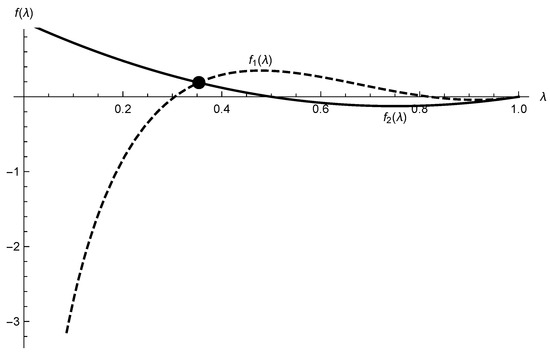
Suppose $\lambda \in (0,1).$ Find λ such that $(8{\lambda }^2-9\lambda +2)log\left(\lambda \right)>2{\lambda }^2-3\lambda +1.$

Solution: An analytical solution of the above inequality is not possible, so we will use numerical algorithms. Let us consider the corresponding equation $(8{\lambda }^2-9\lambda +2)log\left(\lambda \right)=2{\lambda }^2-3\lambda +1.$ Using function Solve in Mathematica software ([11]), we get that $\lambda \approx 0.3536.$ Furthermore, using the function Reduce we see that for $\lambda \in (0.3536,1)$ the inequality holds. The graphical solution is given in Figure 1.

Figure 1. Graphical solution of the inequality $f_1\left(\lambda \right)>f_2\left(\lambda \right),$ where $f_1\left(\lambda \right)=(8{\lambda }^2-9\lambda +2)log\left(\lambda \right)$ and $f_2\left(\lambda \right)=2{\lambda }^2-3\lambda +1$.

Theorem 2. 

The PDF of LiE1 with parameters $\theta >0$ and $\lambda \in (0,1)$ is unimodal if $\lambda \in (0.3536,1).$ Otherwise, it is decreasing.

Proof. 

The first derivative of the logarithm of the PDF $g_1\left(x\right)$ can be represented in the form

$${[log{g}_1\left(x\right)]}^{\prime }=\frac{-\theta s\left(x\right)}{(1-\lambda (1-e^{-\theta x}))(a+b(1-e^{-\theta x}))},$$

where $s\left(x\right)=(a+b)(1-\lambda )-2(a\lambda +b)e^{-\theta x}+\lambda b{e}^{-2\theta x}$, $a=1-\lambda +(3\lambda -2)log\left(\lambda \right)$ and $b=-\lambda (1-\lambda +\lambda log(\lambda \left)\right)$. We transform the function $s\left(x\right)$ to a quadratic function $s\left(y\right)=\lambda b{y}^2-2(b+a\lambda )y+(a+b)(1-\lambda )$, $y\in [0,1]$. Let $y_1$ and $y_2$ represent the roots of the equation $s\left(y\right)=0$. Some calculations indicate that $a>0$, $b<0$, $b+a\lambda >0$ and $a+b>0.$ Thus,

$$\begin{array}{ccc}\hfill y_1+y_2& =& \frac{2(a\lambda +b)}{\lambda b}<0,\hfill \\ \hfill y_1{y}_2& =& \frac{(a+b)(1-\lambda )}{\lambda b}<0,\hfill \end{array}$$

so we have $y_1<0<y_2$ and $\left|y_1\right|>y_2.$ After some calculations, it can be shown that discriminant $D=4{(a\lambda +b)}^2-4\lambda b(1-\lambda )$ is positive and that $s\left(y\right)$ is concave. We need to find when solution $y_2\in (0,1).$ If we set $u=-b$, one gets

$$y_2=\frac{\sqrt{{(a\lambda -u)}^2+\lambda u(a-u)(1-\lambda )}-(a\lambda -u)}{\lambda u}.$$

If $y_2<1$, then

$$\sqrt{{(a\lambda -u)}^2+\lambda u(a-u)(1-\lambda )}<\lambda u+a\lambda -u.$$

(13)

It is not difficult to verify that the right-hand side of the last inequality is positive and we can quadrate (13). Then, the inequality (13) reduces to

$$\lambda u(3\lambda a-u-a)>0.$$

Now, the assertion of the first part of Theorem follows from Example 1.

In case $\lambda <0.3536$, $s\left(y\right)$ is always positive on the interval $(0,1)$, and hence the PDF is decreasing.    □

Different shapes of the PDF in cases of LiE1 model are given in Figure 2.

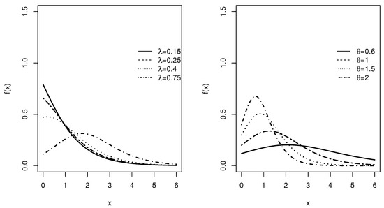
Figure 2. The plots of the density function of the LiE1 distribution for various choices of parameters with $\theta =1$ (left) and $\lambda =0.65$ (right).

The HRF of the LiE1 distribution is

$$h_1\left(x\right)=\frac{\theta [1-\lambda +(3\lambda -2)log\left(\lambda \right)-\lambda (1-\lambda +\lambda log\left(\lambda \right))(1-e^{-\theta x})]}{[1-\lambda (1-e^{-\theta x})][1-2log\left(\lambda \right)-\lambda (1-log\left(\lambda \right))(1-e^{-\theta x})]},x>0,\theta >0,\lambda \in (0,1).$$

Determining the shape of a HRF of a distribution is an important issue in statistical reliability and survival analysis. We give it for the LiE1 model in the following theorem.

Theorem 3. 

The HRF of the LiE1 with parameters $\theta >0$ and $\lambda \in (0,1)$ is an increasing function.

Proof. 

The first derivative of the $log{h}_1\left(x\right)$ can be represented as

$${[log{h}_1\left(x\right)]}^{\prime }=\frac{-\theta e^{-\theta x}s\left(x\right)}{(a+b(1-e^{-\theta x}))(1-\lambda (1-e^{-\theta x}))(d-c(1-e^{-\theta x}))},$$

where a and b were defined in Theorem 2, $c=\lambda (1-log(\lambda \left)\right),$$d=1-2log\left(\lambda \right)$ and $s\left(x\right)=\lambda bc{e}^{-2\theta x}-2\lambda c(a+b)e^{-\theta x}+2\lambda ac-\lambda ad-bd+\lambda cb-ca$. After extensive calculations, it can be shown that $2\lambda ac-\lambda ad-bd+\lambda cb-ca<0.$

Again, using the transformation $y=e^{-\theta x},$ where $y\in [0,1]$, we get quadratic equation $s\left(y\right)=0$ with

$$\begin{array}{ccc}\hfill y_1+y_2& =& \frac{2\lambda c(a+b)}{\lambda b}<0,\hfill \\ \hfill y_1{y}_2& =& \frac{2\lambda ac-\lambda ad-bd+\lambda cb-ca}{\lambda b}>0.\hfill \end{array}$$

Thus, we have $y_1<y_2<0.$ The function $s\left(y\right)$ is concave, and it holds that $s\left(y\right)<0$ for all $y\in [0,1].$ Finally, the HRF is increasing. Hence, we proved Theorem.    □

Different shapes of the HRF in the case of the LiE1 model are outlined in Figure 3.

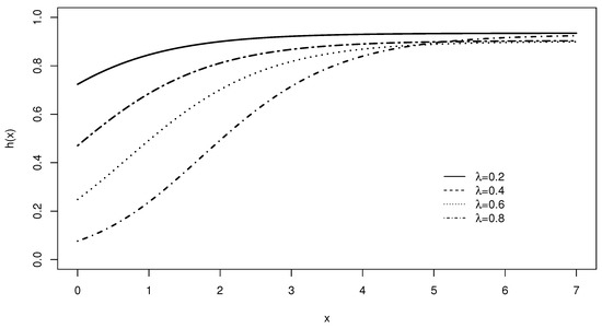
Figure 3. The plots of the HRF of the LiE1 distribution for various choices of parameter $\lambda$ with $\theta =1$.

Now, we will study the shapes of the discrete Lindley exponential distribution of the second kind (LiE2) of distribution. By replacing $\overline{F}\left(x\right)=e^{-\theta x}$ in Equation (11), we obtain the PDF of the LiE2 distribution as

$$g_2(x;\theta ,\lambda )=\frac{\theta e^{-\theta x}[1-\lambda +(3\lambda -2)log\left(\lambda \right)-\lambda (1-\lambda +\lambda log\left(\lambda \right))e^{-\theta x}]}{(1-2log\left(\lambda \right)){(1-\lambda e^{-\theta x})}^3},x>0,\theta >0,\lambda \in (0,1).$$

The shapes of the LiE2 distribution are given by the following theorem.

Theorem 4. 

The PDF of the LiE2 with parameters $\theta >0$ and $\lambda \in (0,1)$ is a decreasing function with ${lim}_{x\to 0}{g}_2\left(x\right)=\frac{\theta (1-\lambda +(\lambda -2)log(\lambda \left)\right)}{{(1-\lambda )}^2(1-2log\left(\lambda \right))}$ and ${lim}_{x\to \infty }g\left(x\right)=0$.

Proof. 

Similarly to in Theorem 2, we have

$${[log{g}_2\left(x\right)]}^{\prime }=\frac{-\theta s\left(x\right)}{(1-\lambda e^{-\theta x})(a+b{e}^{-\theta x})},$$

where $s\left(x\right)=a-4\lambda a{e}^{-\theta x}-3\lambda b\lambda e^{-2\theta x}$, $a=1-\lambda +(3\lambda -2)log\left(\lambda \right)$ and $b=-\lambda (1-\lambda +\lambda log(\lambda \left)\right)$. We can prove that $s\left(x\right)$ is positive for all $x>0$. Letting $y=e^{-\theta x}$, we transform the function $s\left(x\right)$ to a quadratic function $s\left(y\right)=b\lambda y^2+2(b+a\lambda )y+a$; $y\in [0,1]$. Let $y_1<y_2$ represent the roots of the equation $s\left(y\right)=0$. Since we have $a>0$, $b<0$ and $b+a\lambda >0$,

$$\begin{array}{ccc}\hfill y_1+y_2& =& \frac{4a}{3b}<0,\hfill \\ \hfill y_1{y}_2& =& -\frac{a}{3b\lambda }>0,\hfill \end{array}$$

which implies $y_1<y_2<0$. Since $b\lambda <0$ and the discriminant $D=4{(b+a\lambda )}^2-4ab\lambda$ is positive, it follows that $s\left(y\right)$ is concave and positive on $[y_1,y_2]$, which means that $s\left(y\right)$ is positive for $y\in [0,1]$. Finally, $s\left(x\right)$ is positive for all $x>0$ and $g_2^{\prime }\left(x\right)<0$.    □

The HRF of the LiE2 distribution for $x>0,\theta >0,\lambda \in (0,1)$ is given by

$$h_2\left(x\right)=h_2(x;\theta ,\lambda )=\frac{\theta [1-\lambda +(3\lambda -2)log\left(\lambda \right)-\lambda (1-\lambda +\lambda log\left(\lambda \right))e^{-\theta x}]}{[1-\lambda e^{-\theta x}][1-\lambda +(3\lambda -2)log\left(\lambda \right)-\lambda (1-\lambda +(2\lambda -1)log\left(\lambda \right))e^{-\theta x}]}.$$

The shape of the HRF of the LiE2 distribution is given in the following theorem.

Theorem 5. 

The HRF of the LiE2 distribution with parameters $\theta >0$ and $\lambda \in (0,1)$ is an increasing function with ${lim}_{x\to 0}{h}_2\left(x\right)=\frac{\theta (1-\lambda +(\lambda -2)log(\lambda \left)\right)}{{(1-\lambda )}^2(1-2log\left(\lambda \right))}$ and ${lim}_{x\to \infty }{h}_2\left(x\right)=\theta$.

Proof. 

We consider the logarithm of the HRF $h_2\left(x\right)$. Its first derivative can be expressed as

$${[log{h}_2\left(x\right)]}^{\prime }=\frac{-\theta e^{-\theta x}t\left(x\right)}{(a+b{e}^{-\theta x})(1-\lambda e^{-\theta x})(a+c{e}^{-\theta x})},$$

where a and b are defined as in the proof of the previous theorem, $c=-\lambda [1-\lambda +(2\lambda -1)log(\lambda \left)\right]$ and $t\left(x\right)=bc\lambda e^{-2\theta x}+2ac\lambda e^{-\theta x}+a(b+a\lambda -c)$. By letting $y=e^{-\theta x}$, we transform the function $t\left(x\right)$ to the quadratic function $t\left(y\right)=bc\lambda y^2+2ac\lambda y+a(b+a\lambda -c)$; $y\in (0,1)$. As before, let $y_1<y_2$ be the roots of the equation $t\left(y\right)=0$. Some calculations indicate that $a>0$, $b<0$, $c<0$ and $b+a\lambda -c>0$, which implies that

$$\begin{array}{ccc}\hfill y_1+y_2& =& -\frac{2a}{b}>0,\hfill \\ \hfill y_1{y}_2& =& \frac{a(b+a\lambda -c)}{bc\lambda }>0,\hfill \\ \hfill (1-y_1)(1-y_2)& =& 1+\frac{a}{bc\lambda }(b+a\lambda +2c\lambda -c)=1+\frac{a}{bc}[1-3\lambda +2{\lambda }^2-(3-6\lambda +4{\lambda }^2)log\left(\lambda \right)]>0.\hfill \end{array}$$

Thus, two cases can be considered, $0<y_1<y_2<1$ and $1<y_1<y_2$. The first case is not possible, since

$$y_1{y}_2-1=\frac{a(b+a\lambda )-c(a+b\lambda )}{bc\lambda }>0,$$

which follows from the fact that $a+b\lambda ={(1-\lambda )}^2(1+\lambda -(\lambda +2)log\left(\lambda \right))>0$. Thus, $1<y_1<y_2$. Since $bc\lambda >0$ and the discriminant $D=-8ac{\lambda }^3{(1-\lambda )}^2{log}^2\left(\lambda \right)$ is positive, it follows that $t\left(y\right)$ is a convex function and positive on $(0,1)$. This implies that $t\left(x\right)$ is positive for all $x>0$. Finally, $h_2^{\prime }\left(x\right)<0$, which means that the HRF is an increasing function.    □

Using similar calculations, we can derive the shapes of the PDF and HRF of X and Y given by (5), (6), (11) and (12), respectively, under various baseline distributions.

Figure 4 represents plots of the LiE2 density function, while on Figure 5 we have plots of the LiE2 hazard rate functions for various parameter values.

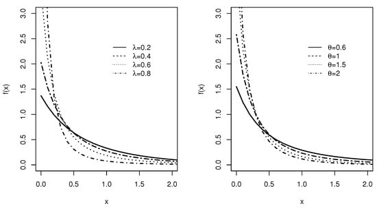
Figure 4. The plots of the density function of the LiE2 distribution for various choices of parameters with $\theta =1$ (left) and $\lambda =0.5$ (right).

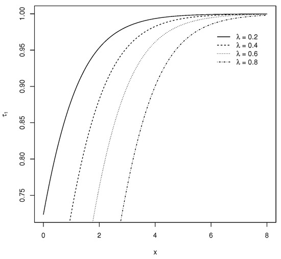
Figure 5. The hazard plots of the LiE2 distribution for various choices of parameter $\lambda$ with $\theta =1$.

Theorem 6. 

The LiE2 distribution function is identifiable with respect to the parameters θ and λ.

Proof. 

As was the case in the proof of Theorem 1, we will assume that $G_2(x;{\theta }_1,{\lambda }_2)=G_2(x;{\theta }_2,{\lambda }_2)$ for all $x>0$ and $F\left(x\right)$ is the CDF of an exponential distribution. As a consequence, we have $h_2(x;{\theta }_1,{\lambda }_2)=h_2(x;{\theta }_2,{\lambda }_2).$ Then, from Theorem 5, we have that ${\theta }_1={\theta }_2$ when $x\to \infty .$ Now, since ${\theta }_1={\theta }_2$ after some algebra, it can be shown that from $h_2(0;{\theta }_1,{\lambda }_2)=h_2(0;{\theta }_2,{\lambda }_2)$ follows ${\lambda }_1={\lambda }_2.$    □

4. Some Mathematical Properties

4.1. Mixture Representations

In this section, we obtain a very useful representation for the LiG1 density function. For $\left|z\right|<1$ and $\rho >0$, we can write

$${(1-z)}^{-\rho }=\sum _{j=0}^{\infty }{w}_j{z}^j,$$

(14)

where $w_j=\Gamma (\rho +j)/[\Gamma \left(\rho \right)j!]$ and $\Gamma \left(\rho \right)={\int }_0^{\infty }{t}^{\rho -1}{\mathrm{e}}^{-t}dt$ is the gamma function. For $\alpha \in (0,1)$, we can apply (14) in Equation (5) to obtain

$$g_1\left(x\right)=f\left(x\right)[a\left(\lambda \right)+b\left(\lambda \right)F\left(x\right)]\sum _{j=0}^{\infty }{v}_{j}F{\left(x\right)}^j,$$

(15)

where $a\left(\lambda \right)=1-\lambda +(3\lambda -2)log\left(\lambda \right)$, $b\left(\lambda \right)=-\lambda [1-\lambda +\lambda log(\lambda \left)\right]$ and

$$v_j=v_j\left(\lambda \right)=\frac{\Gamma (j+3){\lambda }^j}{2(1-2log(\lambda \left)\right)j!}.$$

Henceforth, $T_a$ as a random variable will be said to have the exponentiated-F (“exp-F”) distribution, its power parameter being $a>0$, say, $T_a\sim exp-F\left(a\right)$, if its PDF and CDF are given by

$$\begin{array}{c}\hfill h_a\left(x\right)=af\left(x\right)F^{a-1}\left(x\right)\mathrm{and}{H}_a\left(x\right)=F^a\left(x\right),\end{array}$$

respectively.

Then, using the exp-F distribution, we can write Equation (15) as

$$g_1\left(x\right)=\sum _{j=0}^{\infty }[t_j{h}_{j+1}\left(x\right)+s_j{h}_{j+2}\left(x\right)]=\sum _{j=0}^{\infty }{p}_j{h}_{j+1}\left(x\right),$$

(16)

where $t_j=a\left(\lambda \right)v_j/(j+1)$, $s_j=b\left(\lambda \right)v_j/(j+2)$, $p_j=t_j+s_{j-1}$ (for $j\ge 0$) and $s_{-1}=0$.

Equation (16) is this section’s main result. It shows that the LiF1 family density function is a mixture of $exp-F$ ditributions. Therefore, there are structural properties (for instance incomplete and ordinary moments, generating functions, mean deviations) of the LiF1 family that can be obtained from the corresponding properties of the exp-G distribution. The exp-F mathematical properties have been studied by many authors in recent years, such as Nadarajah and Kotz (2006). In the following sections, we provide some mathematical properties of the LiG1 family distribution.

4.2. Moments

Henceforth, let $T_{j+1}$ have the the exp-F density $h_{j+1}\left(x\right)$ with power parameter $j+1$, say, $T_{j+1}\sim$exp-F$(j+1)$. A first formula for the nth moment of the LiF1 family can be obtained from (16) as

$$\begin{array}{c}\hfill {\displaystyle {\mu }_n^{\prime }=E\left(X^n\right)=\sum _{j=0}^{\infty }{p}_{j}E\left(T_{j+1}^n\right).}\end{array}$$

(17)

Nadarajah and Kotz [12] provide explicit expressions for moments of some exponentiated distributions. They can be used to produce ${\mu }_n^{\prime }$.

A second formula for ${\mu }_n^{\prime }$ can be obtained from (17) in terms of the baseline quantile function (qf) $Q_F\left(u\right)$. We obtain

$$\begin{array}{c}\hfill {\displaystyle {\mu }_n^{\prime }=\sum _{j=0}^{\infty }(j+1)p_j\tau (n,j),}\end{array}$$

(18)

where the integral can be expressed as a function of the F quantile function (qf), say, $Q_F\left(u\right)=F^{-1}\left(u\right)$, as $\tau (n,j)={\int }_0^1{Q}_F{\left(u\right)}^n{u}^{j}du$.

Even though there is an infinite sum in the moments’ equation, it is not difficult to calculate its values. For example, if we set an error to ${10}^{-6}$, then four iterations would be enough for moments’ calculation.

Equations (17) and (18) can be used to directly determine the ordinary moments of some LiF1 distributions. Three examples will be provided here. Here, we consider three examples. LiE1 distribution moments (with scale parameter $\theta >0$ from the exponential baseline distribution) are given by

$${\mu }_n^{\prime }=\frac{n!}{{\theta }^n}\sum _{j=0}^{\infty }\sum _{i=0}^{\infty }\left(\genfrac{}{}{0pt}{}{j}{i}\right){(-1)}^i{p}_j(j+1)\frac{1}{{(i+1)}^{n+1}}.$$

Particularly, we have

$$E\left(X\right)=\sum _{j=0}^{\infty }{p}_j[\psi (j+2)-\psi \left(1\right)],$$

where $\psi (·)$ is the digamma function defined by $\psi (·)={\Gamma }^{{}^{\prime }}(·)/\Gamma (·)$.

For the discrete Lindley Pareto of the first kind (LiPa1) of distribution, the baseline distribution is $F\left(x\right)=1-{(1+x)}^{-\nu }$, $x>0$ and we have

$${\mu }_n^{\prime }=\sum _{j=0}^{\infty }\sum _{i=0}^n\left(\genfrac{}{}{0pt}{}{n}{i}\right){(-1)}^i{p}_j(j+1)B\left(j+1,1-\frac{i}{\nu }\right),\nu >n,$$

where $B(a,b)={\int }_0^1{t}^{a-1}{(1-t)}^{b-1}dt$ is the standard beta function.

For the discrete Lindley standard logistic of the first kind (LiSL1) of distribution, the baseline distribution is $F\left(x\right)={(1+e^{-x})}^{-1}$ and $-\infty <x<\infty$. Using an integral result from [13], we have

$${\mu }_n^{\prime }=\sum _{j=0}^{\infty }\sum _{i=0}^n\left(\genfrac{}{}{0pt}{}{n}{i}\right){(-1)}^{2n-i}\frac{j+1}{\Gamma (j+2)}{p}_j{\Gamma }_{\left(1\right)}^{\left(i\right)}{\Gamma }_{(j+1)}^{(n-i)},$$

where

$${\Gamma }_{\left(a\right)}^{\left(m\right)}={\int }_0^{\infty }{(lnx)}^m{x}^{a-1}{e}^{-x}dx.$$

Further, central moments, that is, moments around the mean, can also be computed. The relation between the central moments (${\mu }_r$) and the moments about the origin are given by

$${\displaystyle {\mu }_r=\sum _{k=0}^r{(-1)}^k\left(\genfrac{}{}{0pt}{}{r}{k}\right){\left({\mu }_1^{\prime }\right)}^k{\mu }_{r-k}^{\prime }.}$$

The cumulants of the distribution can also be computed together with the skewness and kurtosis measures. For this approach, we refer the reader to [14]. The skewness and kurtosis plots for these distributions are sketched in Figure 6, Figure 7, Figure 8 and Figure 9. We observe that various skewness and kurtosis values can be obtained from these models.

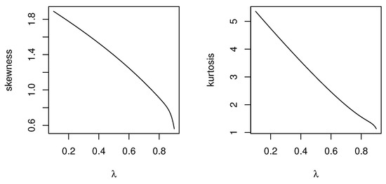
Figure 6. Skewness and kurtosis plots of the LiE1 distribution as a function of parameter $\lambda$.

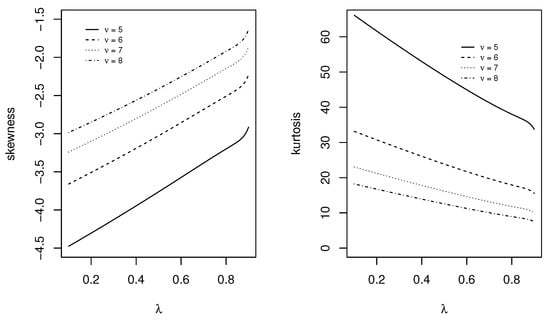
Figure 7. Skewness and kurtosis plots of the LiPa1 distribution as a function of parameter $\lambda$.

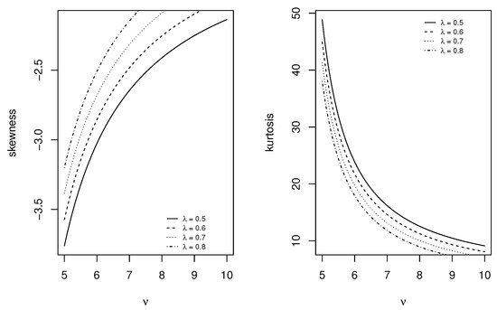
Figure 8. Skewness and kurtosis plots of the LiPa1 distribution as a function of parameter $\nu$.

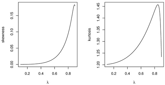
Figure 9. Skewness and kurtosis plots of the LiSL1 distribution as a function of parameter $\lambda$.

4.3. Generating Function

As far as the moment generating function (mgf) $M\left(t\right)=E\left(e^{tX}\right)$ of X is concerned, we will provide two formulae. The first $M\left(t\right)$ formula comes from (16) as

$$\begin{array}{c}\hfill {\displaystyle M\left(t\right)=\sum _{j=0}^{\infty }{p}_j{M}_{j+1}\left(t\right),}\end{array}$$

(19)

where $M_{j+1}\left(t\right)$ is the mgf of $T_{j+1}$. Therefore, $M\left(t\right)$ is determined by the generating function of the $exp-F(j+1)$ distribution. The second M(t) formula is derived from (16)

$$\begin{array}{c}\hfill {\displaystyle M\left(t\right)=\sum _{j=0}^{\infty }(j+1)p_j\rho (t,j),}\end{array}$$

(20)

where $\rho (t,j)$ can be calculated from $Q_F\left(x\right)$ as

$$\begin{array}{c}\hfill {\displaystyle \rho (t,j)={\int }_0^{1}exp\left\{t{Q}_G\left(u\right)\right\}{u}^{j}du.}\end{array}$$

(21)

It is possible to get several mgf of some LiG1 distributions using Equations (20) and (21), which can be used to directly obtain the mgf of several LiG1 distributions. For example, we have the mgfs of the LiE1 (with parameter $\lambda$) and and LiSL1 as

$$\begin{array}{c}\hfill {\displaystyle M\left(t\right)=\sum _{j=0}^{\infty }(j+1)B(j+1,1-\lambda t)p_j,t>\lambda ,}\end{array}$$

and

$$\begin{array}{c}\hfill {\displaystyle M\left(t\right)=\sum _{j=0}^{\infty }(j+1)B(t+j+1,1-t)p_j,t<1,}\end{array}$$

respectively.

4.4. Incomplete Moments and Mean Deviations

The shapes of many of the distributions can, for empirical reasons, be conveniently described as incomplete moments. Such moments are important in measuring inequality, such as income quantiles and Lorenz and Bonferroni curves, which depend on the distribution incomplete moments. The $n-$th incomplete moment of the random variable X is defined as

$$\begin{array}{c}\hfill {\displaystyle m_n\left(y\right)={\int }_0^y{g}_1\left(x\right)dx=\sum _{j=0}^{\infty }(j+1){\int }_0^{F\left(y\right)}{Q}_F{\left(u\right)}^n{u}^{j}du.}\end{array}$$

(22)

The integral in (22) can be computed in the closed-form for several baseline F distributions.

The mean deviations about the mean (${\delta }_1=E\left(\right|X-{\mu }_1^{\prime }\left|\right)$) and about the median (${\delta }_2=E\left(\right|X-M\left|\right)$) of X can be expressed as ${\delta }_1=2{\mu }_1^{\prime }{G}_1\left({\mu }_1^{\prime }\right)-2m_1\left({\mu }_1^{\prime }\right)$ and ${\delta }_2={\mu }_1^{\prime }-2m_1\left(M\right)$, respectively, where ${\mu }_1^{\prime }=E\left(X\right)$, $M=Median\left(X\right)$ is the median of X computed from

$$G_1\left(M\right)=\frac{F\left(M\right)\{1-\lambda +(3\lambda -2)log(\lambda )-\lambda [1-\lambda +(2\lambda -1)log\left(\lambda \right)\left]F\right(x\left)\right\}}{[1-2log\left(\lambda \right)]{[1-\lambda F\left(M\right)]}^2}=0.5,$$

$G_1\left({\mu }_1^{\prime }\right)$ is easily calculated from (4) and $m_1\left(z\right)={\int }_{-\infty }^{z}xf\left(x\right)dx$ is the first exp-F incomplete moment.

We will provide two ways to compute $delt{a}_1$ and $delt{a}_2$. In the first instance, we can derive a general equation for $m_1\left(z\right)$ from (16) by setting $u=F\left(x\right)$ as

$$\begin{array}{c}\hfill {\displaystyle m_1\left(z\right)=\sum _{j=0}^{\infty }(j+1)A_j\left(z\right),}\end{array}$$

(23)

where

$$\begin{array}{c}\hfill {\displaystyle A_j\left(z\right)={\int }_{-\infty }^{z}x{h}_{j+1}\left(x\right)dx={\int }_0^{F\left(z\right)}{Q}_F\left(u\right)u^{j}du.}\end{array}$$

(24)

Equation (24) provides the basic quantity for computing the mean deviations of the exp-F distributions. Hence, the mean deviations ${\delta }_1$ and ${\delta }_2$ depend only on the exp-F mean deviations. Thus, alternative representations for ${\delta }_1$ and ${\delta }_2$ are given by ${\delta }_1=2{\mu }_1^{\prime }{G}_1\left({\mu }_1^{\prime }\right)-2{\sum }_{j=0}^{\infty }(j+1)A_j\left({\mu }_1^{\prime }\right)$ and ${\delta }_2={\mu }_1^{\prime }-2{\sum }_{j=0}^{\infty }(j+1)A_j\left(M\right)$.

In a similar way, the mean deviations of any LiF1 distribution can be computed from Equations (23) and (24). For example, the mean deviations of the LiE1 (with parameter $\lambda$), LiPa1 (with parameter $0<\nu <1$) and LiSL1 are determined immediately (by using the generalized binomial expansion) from the functions

$$\begin{array}{c}\hfill A_j\left(z\right)={\lambda }^{-1}\Gamma \left(j\right)\sum _{m=0}^{\infty }\frac{{\displaystyle {(-1)}^m\{1-exp(-m\lambda z)\}}}{\Gamma (j-m)(m+1)!},\end{array}$$

and

$$\begin{array}{c}\hfill {\displaystyle A_j\left(z\right)=\sum _{m=0}^{\infty }\sum _{r=0}^m\frac{{(-1)}^m}{(1-r\nu )}\left(\genfrac{}{}{0pt}{}{j+1}{m}\right)\left(\genfrac{}{}{0pt}{}{m}{r}\right)z^{1-r\nu },}\end{array}$$

and

$$\begin{array}{c}\hfill {\displaystyle A_j\left(z\right)=\frac{1}{\Gamma \left(j\right)}\sum _{m=0}^{\infty }\frac{{(-1)}^m\Gamma (j+m+1)\{1-exp(-mz)\}}{{\displaystyle (m+1)!}},}\end{array}$$

respectively.

Bonferroni and Lorenz curves defined can be given to obtain for a given probability $\pi$ by $B\left(\pi \right)=T\left(q\right)/\left(\pi {\mu }_1^{\prime }\right)$ and $L\left(\pi \right)=T\left(q\right)/{\mu }_1^{\prime }$, respectively, where ${\mu }_1^{\prime }=E\left(X\right)$ and $q=Q\left(\pi \right)$ is the LiG1-F qf at $\pi .$

5. On the Maximum-Likelihood Estimation of Parameters

We propose to use the maximum likelihood (ML) estimation method for the parameter estimation of the introduced distributions. The log-likelihood function for the general case (5) is given by

$$\begin{array}{cc}\hfill \mathcal{L}(\lambda ,\psi )& =-nlog(1-2log\left(\lambda \right))-3\sum _{i=1}^{n}log(1-\lambda F(x_i;\psi ))+\sum _{i=1}^{n}logf(x_i;\psi )\hfill \\ \hfill & +\sum _{i=1}^{n}log\left[1-\lambda +(3\lambda -2)log\left(\lambda \right)-\lambda (1-\lambda +\lambda log\left(\lambda \right))F(x_i;\psi )\right].\hfill \end{array}$$

In this special case, we consider the exponential baseline distribution. Thus, for the LiE1 model, the estimating equations are given by   

$$\begin{array}{cc}\hfill & \frac{\mathcal{L}(\lambda ,\theta )}{\partial \theta }=3\lambda \theta \sum _{i=1}^n\frac{e^{-\theta x_i}}{1-\lambda (1-e^{-\theta x_i})}+b\theta \sum _{i=1}^n\frac{e^{-\theta x_i}}{a+b(1-e^{\theta x_i})}+\frac{n}{\theta }-\sum _{i=1}^n{x}_i=0\hfill \\ \hfill & \frac{\mathcal{L}(\lambda ,\theta )}{\partial \lambda }=3\sum _{i=1}^n\frac{1-e^{-x_i\theta }}{1-\lambda (1-e^{-x_i\theta })}+\frac{2n}{\lambda (1-2log(\lambda \left)\right)}\hfill \end{array}$$

(25)

$$\begin{array}{cc}\hfill & +\sum _{i=1}^n\frac{2-\frac{2}{\lambda }+3log\left(\lambda \right)-(1-e^{-x_i\theta })\lambda log\left(\lambda \right)-(1-e^{-x_i\theta })(1-\lambda +\lambda log\left(\lambda \right))}{1-\lambda +(-2+3\lambda )log\left(\lambda \right)-(1-e^{-x_i\theta })(1-\lambda +\lambda log\left(\lambda \right))}=0.\hfill \end{array}$$

(26)

Now, we will study the existence of the ML estimators when the other parameter is known in advance (or given).

Theorem 7. 

If the parameter λ is known, then the Equation (25) has at least one root in the interval $(0,+\infty ).$

Proof. 

One can readily verify that $\underset{\theta \to +\infty }{lim}\frac{\mathcal{L}(\lambda ,\theta )}{\partial \theta }=-{\displaystyle \sum _{i=1}^n}{x}_i$ and $\underset{\theta \to 0+0}{lim}\frac{\mathcal{L}(\lambda ,\theta )}{\partial \theta }=+\infty .$ Thus, there exists at least one root of the Equation (25).    □

Theorem 8. 

Assuming that

$$\begin{array}{c}\hfill \sum _{i=1}^n{e}^{-x_i\theta }<\frac{n}{2}\end{array}$$

and if the parameter θ is known, then (26) has at least one root on the interval $(0,1).$

Proof. 

Applying L’Hôpital’s rule, we get $\underset{\lambda \to 1-0}{lim}\frac{\mathcal{L}(\lambda ,\theta )}{\partial \lambda }=-\infty$ and $\underset{\lambda \to 0+0}{lim}\frac{\mathcal{L}(\lambda ,\theta )}{\partial \lambda }=3{\displaystyle \sum _{i=1}^n}(1-e^{-x_i\theta })-\frac{3n}{2}.$

In order to have at least one solution, it is necessary to have $3{\displaystyle \sum _{i=1}^n}(1-e^{-x_i\theta })-\frac{3n}{2}>0$. Hence the theorem.    □

On the other hand, the estimating equations for the LiE2 model are given by

$$\begin{array}{ccc}\hfill \frac{\mathcal{L}(\lambda ,\theta )}{\partial \theta }& =& -3\lambda \theta \sum _{i=1}^n\frac{e^{-\theta x_i}}{1-\lambda e^{-\theta x_i}}-b\theta \sum _{i=1}^n\frac{e^{-\theta x_i}}{a+b{e}^{\theta x_i}}+\frac{n}{\theta }-\sum _{i=1}^n{x}_i=0\hfill \\ \hfill \frac{\mathcal{L}(\lambda ,\theta )}{\partial \lambda }& =& 3\sum _{i=1}^n\frac{e^{-x_i\theta }}{1-\lambda e^{-x_i\theta }}+\frac{2n}{\lambda (1-2log(\lambda \left)\right)}\hfill \end{array}$$

(27)

$$\begin{array}{ccc}& +& \sum _{i=1}^n\frac{2-\frac{2}{\lambda }+3log\left(\lambda \right)-e^{-x_i\theta }\lambda log\left(\lambda \right)-e^{-x_i\theta }(1-\lambda +\lambda log\left(\lambda \right))}{1-\lambda +(-2+3\lambda )log\left(\lambda \right)-e^{-x_i\theta }(1-\lambda +\lambda log\left(\lambda \right))}=0.\hfill \end{array}$$

(28)

The next two theorems examine the existence problem of the ML estimates via (27) and (28). Their proofs are very similar to those cases of Theorems 7 and 8, so we here omit them.

Theorem 9. 

If the parameter λ is known, then the Equation (27) has at least one root on the interval $(0,+\infty ).$

Theorem 10. 

If the parameter θ is known and if it is assumed that

$$\begin{array}{c}\hfill \sum _{i=1}^n{e}^{-x_i\theta }>\frac{n}{2},\end{array}$$

then the Equation (28) has at least one root on the interval $(0,1).$

Clearly, the log-likelihood estimating equations for the parameters are nonlinear in the sense that the estimators cannot be obtained in closed forms. Thus, a numerical iterative method such as the Newton–Raphson one should be used in the estimation.

6. Estimation of Parameters via the EM Algorithm

We propose to use the method of maximum likelihood in estimating the parameters of the introduced models. The construction method of the models suggests using an EM (expectation maximization) algorithm. In this section, we provide EM algorithms for the estimation of the unknown parameters $\theta$ and $\lambda$ for both exponential-discrete Lindley distributions.

6.1. EM Algorithm for the LiE1 Model

The missing data random variable will be the random variable M with the zero-truncated discrete Lindley distribution. Let us derive its probability mass function as

$$\begin{array}{cc}\hfill P(M=m)& =\frac{P(N=m)}{1-P(N=0)}\hfill \\ \hfill & =\frac{{\lambda }^{m-1}[\lambda log\left(\lambda \right)+(1-\lambda )(1-(m+1)log\left(\lambda \right))]}{1-2log\left(\lambda \right)},m=1,2,\cdots ,\hfill \end{array}$$

where N is a random variable with the discrete Lindley distribution with the parameter $\lambda \in (0,1)$. Next, the random variable $X=max(Z_1,\cdots ,Z_M)$ for a given $M=m$ has the CDF ${(1-e^{-\theta x})}^m$. Then, the PDF of the complete-data distribution is given by

$$f(x,m)=\frac{\theta m{\lambda }^{m-1}\left\{\lambda log\left(\lambda \right)+(1-\lambda )[1-(m+1)log(\lambda \left)\right]\right\}{e}^{-\theta x}{(1-e^{-\theta x})}^{m-1}}{1-2log\left(\lambda \right)}.$$

The marginal PDF of X is given by

$$f_X\left(x\right)=\frac{\theta e^{-\theta x}\left\{1-\lambda +(3\lambda -2)log\left(\lambda \right)-(1-e^{-\theta x})\lambda [\lambda (log\left(\lambda \right)-1)+1]\right\}}{(1-2log\left(\lambda \right)){[1-(1-e^{-\theta x})\lambda ]}^3}.$$

Then, the conditional PDF of M for given $X=x$ is given by

$$f_{M|X}\left(m\right|x)=\frac{m{(1-e^{-\theta x})}^{m-1}{\lambda }^{m-1}{[1-(1-e^{-\theta x})\lambda ]}^3\left\{\lambda log\left(\lambda \right)+(1-\lambda )[1-(m+1)log(\lambda \left)\right]\right\}}{1-\lambda +(3\lambda -2)log\left(\lambda \right)-(1-e^{-\theta x})\lambda [\lambda (log\left(\lambda \right)-1)+1]},$$

where $m=1,2,3,\dots$.

The E-step of the EM algorithm requires the computation of the conditional expectation of the random variable M for a given $X=x$. Now, we have

$$\begin{array}{cc}\hfill & E\left(M\right|X)=\hfill \\ \hfill & =\frac{\lambda log\left(\lambda \right)(3-{\xi }^2(x;\lambda ,\theta )+4\xi (x;\lambda ,\theta ))-(4\xi (x;\lambda ,\theta )+2)log\left(\lambda \right)+(1-\lambda )(1-{\xi }^2(x;\lambda ,\theta ))}{(1-\xi (x;\lambda ,\theta ))\left\{1-\lambda +(3\lambda -2)log\left(\lambda \right)-\xi (x;\lambda ,\theta )\left[\lambda \right(log\left(\lambda \right)-1)+1]\right\}},\hfill \end{array}$$

where $\xi (x;\lambda ,\theta )=\lambda (1-e^{-\theta x})$.

In the M-step, we consider the complete data log-likelihood function, which is given by

$$\begin{array}{cc}\hfill l_c(\theta ,\lambda )& =nlog\left(\theta \right)+\sum _{i=1}^{n}log\left(m_i\right)-\theta \sum _{i=1}^n{x}_i+\sum _{i=1}^n(m_i-1)log(1-e^{-\theta x_i})+\left(\sum _{i=1}^n{m}_i-n\right)log\left(\lambda \right)\hfill \\ \hfill & +\sum _{i=1}^{n}log\{\lambda log\left(\lambda \right)+(1-\lambda )[1-(m_i+1)log\left(\lambda \right)]\}-nlog(1-2log\left(\lambda \right)).\hfill \end{array}$$

Maximizing the log-likelihood function $l_c(\theta ,\lambda )$, the obtained estimates in the $k+1$ iteration are given by   

$${\theta }^{(k+1)}=n{\left\{n\overline{x}-\sum _{i=1}^n\frac{x_i(m_i^{(k+1)}-1)e^{-{\theta }^{(k+1)}{x}_i}}{1-e^{-{\theta }^{(k+1)}{x}_i}}\right\}}^{-1}$$

$$\begin{array}{cc}\hfill {\lambda }^{(k+1)}& =\left[\frac{n(1+2log\left({\lambda }^{(k+1)}\right))}{2log\left({\lambda }^{(k+1)}\right)-1}-\sum _{i=1}^n{m}_i^{(k+1)}\right]\hfill \\ \hfill & \times {\left\{\sum _{i=1}^n\frac{(m_i+2)log\left({\lambda }^{(k+1)}\right)-((1-{\lambda }^{(k+1)})/{\lambda }^{(k+1)})(m_i^{(k+1)}+1)}{{\lambda }^{(k+1)}log\left({\lambda }^{(k+1)}\right)+(1-{\lambda }^{(k+1)})\left[1-(m_i^{(k+1)}+1)log\left({\lambda }^{(k+1)}\right)\right]}\right\}}^{-1},\hfill \end{array}$$

where $\overline{x}$ is the sample mean and

$$\begin{array}{cc}\hfill m_i^{(k+1)}& =\left\{{\lambda }^{\left(k\right)}log\left({\lambda }^{\left(k\right)}\right)(3-{\xi }^2(x_i;{\lambda }^{\left(k\right)},{\theta }^{\left(k\right)})+4\xi (x_i;{\lambda }^{\left(k\right)},{\theta }^{\left(k\right)}))-(4\xi (x_i;{\lambda }^{\left(k\right)},{\theta }^{\left(k\right)})+2)log\left({\lambda }^{\left(k\right)}\right)\right.\hfill \\ \hfill & \left.+(1-{\lambda }^{\left(k\right)})(1-{\xi }^2(x_i;{\lambda }^{\left(k\right)},{\theta }^{\left(k\right)}))\right\}/\left\{(1-\xi (x_i;{\lambda }^{\left(k\right)},{\theta }^{\left(k\right)}))\left[1-{\lambda }^{\left(k\right)}+(3{\lambda }^{\left(k\right)}-2)log\left({\lambda }^{\left(k\right)}\right)\right.\right.\hfill \\ \hfill & \left.\left.-\xi (x_i;{\lambda }^{\left(k\right)},{\theta }^{\left(k\right)})\left({\lambda }^{\left(k\right)}(log\left({\lambda }^{\left(k\right)}\right)-1)+1\right)\right]\right\}.\hfill \end{array}$$

The solutions for these equations can be found using an iterative numerical process. For example, one can use the uniroot function in R (R Core Team, 2020).

6.2. EM Algorithm for the LiE2 Model

In this case, the random variable $Y=min(Z_1,\cdots ,Z_M)$ for a given $M=m$ has the exponential distribution with the scale parameter $\theta m$. Thus, the PDF of the hypothetical complete-data distribution is

$$f(y,m)=\frac{{\lambda }^{m-1}[\lambda log\left(\lambda \right)+(1-\lambda )(1-(m+1)log\left(\lambda \right))]\theta m{e}^{-\theta my}}{1-2log\left(\lambda \right)},y>0,m=1,2,\cdots$$

Following some calculations, we can deduce that the marginal PDF of the random variable Y is given by

$$f\left(y\right)=\frac{\theta e^{-\theta y}[1-\lambda +(3\lambda -2)log\left(\lambda \right)-\lambda (1-\lambda +\lambda log\left(\lambda \right))e^{-\theta y}]}{(1-2log\left(\lambda \right)){(1-\lambda e^{-\theta y})}^3},y>0,$$

which implies that the conditional PDF of M for given $Y=y$ has the form

$$f_{M|Y}\left(m\right|y)=\frac{m{\lambda }^{m-1}{e}^{-\theta (m-1)y}{(1-\lambda e^{-\theta y})}^3[\lambda log\left(\lambda \right)+(1-\lambda )(1-(m+1)log\left(\lambda \right))]}{1-\lambda +(3\lambda -2)log\left(\lambda \right)-\lambda (1-\lambda +\lambda log\left(\lambda \right))e^{-\theta y}},m=1,2,\cdots$$

The E-step of the EM algorithm requires the computation of the conditional expectation of the random variable M for a given $Y=y$. We have that

$$E\left(M\right|Y=y)=\frac{1-\lambda +(3\lambda -2)log\left(\lambda \right)-4(1-\lambda )\lambda e^{-\theta y}log\left(\lambda \right)-{\lambda }^2(1-\lambda +\lambda log\left(\lambda \right))e^{-2\theta y}}{(1-\lambda e^{-\theta y})(1-\lambda +(3\lambda -2)log\left(\lambda \right)-\lambda (1-\lambda +\lambda log\left(\lambda \right))e^{-\theta y})}.$$

In the M-step, we need the complete data log-likelihood function, which is given by

$$\begin{array}{ccc}\hfill l_c(\theta ,\lambda )& =& nlog\left(\theta \right)+\sum _{i=1}^{n}log\left(m_i\right)-\theta \sum _{i=1}^n{m}_i{y}_i+\left(\sum _{i=1}^n{m}_i-n\right)log\left(\lambda \right)\hfill \\ & & +\sum _{i=1}^{n}log[\lambda log\lambda +(1-\lambda )(1-(m_i+1)log\left(\lambda \right))]-nlog(1-2log\left(\lambda \right)).\hfill \end{array}$$

By maximizing the log-likelihood function $l_c(\theta ,\lambda )$, we obtain the estimates in the $k+1$ iteration as follows:   

$${\theta }^{(k+1)}=\frac{n}{{\sum }_{i=1}^n{y}_i{m}_i^{(k+1)}},$$

$$\begin{array}{cc}\hfill & \sum _{i=1}^n\frac{{\lambda }^{(k+1)}(m_i^{(k+1)}+2)log\left({\lambda }^{(k+1)}\right)-(1-{\lambda }^{(k+1)})(1+m_i^{(k+1)})}{{\lambda }^{(k+1)}log\left({\lambda }^{(k+1)}\right)+(1-{\lambda }^{(k+1)})(1-(m_i^{(k+1)}+1)log\left({\lambda }^{(k+1)}\right))}+\frac{2n}{1-2log\left({\lambda }^{(k+1)}\right)}=\hfill \\ & =n-\sum _{i=1}^n{m}_i^{(k+1)},\hfill \end{array}$$

where

$$\begin{array}{cc}\hfill m_i^{(k+1)}& =\left\{1-{\lambda }^{\left(k\right)}+(3{\lambda }^{\left(k\right)}-2)log\left({\lambda }^{\left(k\right)}\right)-4(1-{\lambda }^{\left(k\right)}){\lambda }^{\left(k\right)}log\left({\lambda }^{\left(k\right)}\right)e^{-{\theta }^{\left(k\right)}{y}_i}-{\lambda }^{2\left(k\right)}(1-{\lambda }^{\left(k\right)}\right.\hfill \\ \hfill & \left.+{\lambda }^{\left(k\right)}log\left({\lambda }^{\left(k\right)}\right))e^{-2{\theta }^{\left(k\right)}{y}_i}\right\}/\left\{(1-{\lambda }^{\left(k\right)}{e}^{-{\theta }^{\left(k\right)}{y}_i})(1-{\lambda }^{\left(k\right)}+(3{\lambda }^{\left(k\right)}-2)log\left({\lambda }^{\left(k\right)}\right)\right.\hfill \\ \hfill & \left.-{\lambda }^{\left(k\right)}(1-{\lambda }^{\left(k\right)}+{\lambda }^{\left(k\right)}log\left({\lambda }^{\left(k\right)}\right))e^{-{\theta }^{\left(k\right)}{y}_i})\right\}.\hfill \end{array}$$

7. Simulation Study

In this section, we consider LiE1 and LiE2 models and present a simulation study testing the performances of the estimators using the EM algorithm. We generated 10,000 random samples in batches of 50, 100 and 200 from both models.

We can generate random numbers from the $LiE1$ distribution by using the inverse transform method. Let u be a random number from the uniform distribution on $[0,1]$. Employing some algebra, we have $x=-log(1-y)/\theta$, a number from the $LiE1$ distribution. Here,

$$y=\frac{2\lambda au+c-\sqrt{{\Delta }_1}}{2(b+{\lambda }^{2}au)},$$

where $a=1-2log\left(\lambda \right)$, $b=\lambda [1-\lambda +(2\lambda -1)log(\lambda \left)\right]$, $c=1-\lambda +(3\lambda -2)log\left(\lambda \right)$ and ${\Delta }_1={(2\lambda au+c)}^2-4({\lambda }^{2}au+b)au$.

Similarly, we can generate random numbers from the $LiE2$ distribution by using the inverse transform method. Let u be a random number from the uniform distribution on $[0,1]$. Following some calculations, we have $y=-log\left(x\right)/\theta$, a number from the $LiE2$ distribution. Here,

$$x=\frac{d+a(1-2u\lambda )-\sqrt{{\Delta }_2}}{2(d-{\lambda }^{2}au)},$$

where $d=\lambda [1-log(\lambda \left)\right]$ and ${\Delta }_2={[(2u\lambda -1)a-d]}^2-4a(d-ua{\lambda }^2)(1-u)$.

We used R (R Core Team, 2020) with uniroot to run the EM algorithms. We took the parameter values as the starting points for the iterations in the algorithms. The algorithms stopped when $|{\lambda }^{(k+1)}-{\lambda }^{\left(k\right)}|<{10}^{-5}$. The simulation results of the empirical means and mean square errors (MSEs) are reported in Table 1 and Table 2. We observe that the estimates are close to the parameter values and the MSEs decrease with increasing sample size. This makes the use of the EM algorithm plausible for estimation.

Table 1. Empirical means and MSEs of the maximum-likelihood estimates of the LiE1 for different values of the parameters.

n	$\mathit{\lambda }$	$\mathit{\theta }$	$\widehat{\mathit{\lambda }}$	$\widehat{\mathit{\theta }}$	$\mathit{\lambda }$	$\mathit{\theta }$	$\widehat{\mathit{\lambda }}$	$\widehat{\mathit{\theta }}$	$\mathit{\lambda }$	$\mathit{\theta }$	$\widehat{\mathit{\lambda }}$	$\widehat{\mathit{\theta }}$
50	0.6	0.5	0.5954	0.5159	0.6	1	0.5963	1.0350	0.6	2	0.5965	2.0675
			(0.0163)	(0.0089)			(0.0161)	(0.0369)			(0.0159)	(0.1448)
100			0.5952	0.5068			0.5957	1.0143			0.5952	2.0264
			(0.0081)	(0.0041)			(0.0080)	(0.0164)			(0.0082)	(0.0685)
200			0.5954	0.5020			0.5970	1.0067			0.5949	2.0058
			(0.0040)	(0.0020)			(0.0041)	(0.0083)			(0.0040)	(0.0334)

Table 2. Empirical means and the MSEs of the maximum-likelihood estimates of the LiE2 for different values of the parameters.

n	$\mathit{\lambda }$	$\mathit{\theta }$	$\widehat{\mathit{\lambda }}$	$\widehat{\mathit{\theta }}$	$\mathit{\lambda }$	$\mathit{\theta }$	$\widehat{\mathit{\lambda }}$	$\widehat{\mathit{\theta }}$	$\mathit{\lambda }$	$\mathit{\theta }$	$\widehat{\mathit{\lambda }}$	$\widehat{\mathit{\theta }}$
50	0.6	0.2	0.5335	0.2379	0.6	1	0.5344	1.1898	0.8	1	0.6883	1.7007
			(0.0368)	(0.0119)			(0.0375)	(0.2993)		(0.0434)	(1.7356)
100			0.5526	0.2252			0.5455	1.1424		0.7331	1.4154
			(0.0240)	(0.0068)			(0.0248)	(0.1737)		(0.0213)	(0.7965)
200			0.5668	0.2176			0.5669	1.0838		0.7616	1.2371
			(0.0127)	(0.0036)			(0.0128)	(0.0884)		(0.0093)	(0.3335)

8. Real Data Fitting

In this section, we investigate the performance of the introduced distributions in data fitting. We also compare them with their natural competitor, that is, the generalized exponential (GE) distribution studied in [15]. The GE distribution was proposed as an alternative to exponential, gamma and Weibull distributions. A lot of work in the literature has shown that it is a flexible model with reverse J-shaped and positively skewed unimodal data fitting. The PDF of the GE distribution is given by

$$f(x;\alpha ,\theta )=\alpha \theta e^{-\theta x}{(1-e^{-\theta x})}^{\alpha -1},x,\alpha ,\beta >0.$$

We consider the maximum likelihood method in the estimation. Since we compare the models, we used the direct maximization of the respective log-likelihood functions.

8.1. Carbon Data Set

Let us consider a data set (uncensored) from [16], which includes 100 observations regarding breaking stress of carbon fibers in Gba. The data are given in Table 3.

Table 3. Data on the breaking stress of carbon fibers.

0.39	0.81	0.85	0.98	1.08	1.12	1.17	1.18	1.22	1.25
1.36	1.41	1.47	1.57	1.57	1.59	1.59	1.61	1.61	1.69
1.69	1.71	1.73	1.80	1.84	1.84	1.87	1.89	1.92	2.00
2.03	2.03	2.05	2.12	2.17	2.17	2.17	2.35	2.38	2.41
2.43	2.48	2.48	2.50	2.53	2.55	2.55	2.56	2.59	2.67
2.73	2.74	2.76	2.77	2.79	2.81	2.82	2.83	2.85	2.87
2.88	2.93	2.95	2.96	2.97	2.97	3.09	3.11	3.11	3.15
3.15	3.19	3.19	3.22	3.22	3.27	3.28	3.31	3.31	3.33
3.39	3.39	3.51	3.56	3.60	3.65	3.68	3.70	3.75	4.20
4.38	4.42	4.70	4.90	4.91	5.08	5.56

The data were also used in [17].

We used the LiE1 distribution in fitting instead of LiE2, since the data exhibits a unimodal shape (see Figure 10). One can also use the total time test (TTT) plot procedure to determine an appropriate model shape.

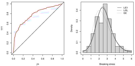
Figure 10. TTT plot of the data set (on the left) and several fits for the Carbon data (on the right).

The TTT plots were introduced by [18] for model identification purposes, that is, for choosing a suitable lifetime distribution. These plots were studied in detail by [19]. Let $x_{\left(1\right)}\le \cdots \le x_{\left(n\right)}$ denote the ordered observations from the random sample of size n. The TTT plot is obtained in the following way:

• Let $s_0=0$.
• Calculate the TTT values $s_j=s_{j-1}+(n-j+1)(x_{\left(j\right)}-x_{(j-1)})$ for $j=1,2,\dots ,n$.
• Obtain the normalized TTT values by $u_j=s_j/s_n$ for $j=0,1,2,\dots ,n$.
• Plot the points $(j/n,u_j)$ for $j=0,1,2,\dots ,n$, and then join them by line segments.

A TTT plot is a diagnostic tool in the sense that it gives an insight about the aging properties of the underlying distribution. Then, one can choose an appropriate lifetime distribution for modeling the data. For example, when the $TTT$ plot is concave, a life distribution with an increasing failure rate should be used. The TTT plot for the Carbon data set is sketched in the lhs of Figure 10. It can be seen that it is concave. Thus, a model with increasing failure rate like LiE1 should be used.

Further, the HRF can not only be increasing, but also be constant, decreasing or even a U-shaped. These futures may also be inferred from the TTT plot. The HRF is constant when the TTT plot is straight diagonal, decreases when the TTT plot is convex and is U-shaped if the TTT plot is S-shaped—that is, first convex and then changed to a concave shape. When the ordering is reversed in the S-shaped case, a HRF with a unimodal characteristic is obtained.

Alternatively, we also fit LiSL1 and GE distributions to this data set and computed the parameter estimates using the optim function in R [20]. The results are reported in Table 4. We observe that the Lie1 distribution is better than the others according to the Akaike information criterion (AIC). The Kolmogorov–Simirnov test statistic was 0.074605 with p-value 0.6338. Figure 10 also supports this good fit. On the other hand, the EM algorithm gave $\widehat{\lambda }=0.9415187$ and $\widehat{\theta }=1.432148$, which are similar values to those obtained from direct maximization.

Table 4. Maximum-likelihood estimates with standard errors in parentheses, log-likelihood and AIC values for Carbon data.

Model	$\widehat{\mathit{\lambda }}$	$\widehat{\mathit{\theta }}$	$\widehat{\mathit{\alpha }}$	log-lik	AIC
LiE1	0.9419	1.4344		−142.1633	288.3266
	(0.0169)	(0.1187)
LiSL1	0.9528	1.5067		−142.9535	289.9069
	(0.0127)	(0.1109)
GE		1.0132	7.7883	−146.1823	296.3646
		(0.0875)	(1.4962)

8.2. Failure Data Set

The data set is based on the number of successive failures of air conditioning systems on 13 Boeing 720 air planes. The data set is from [21] and was recently analyzed in [22]. Since the data exhibit a reversed J-shape (see Figure 11), we used the LiE2 distribution in fitting. TTT plot sketched in the lhs of Figure 11 also supports this conjecture, since it produces a convex shape.

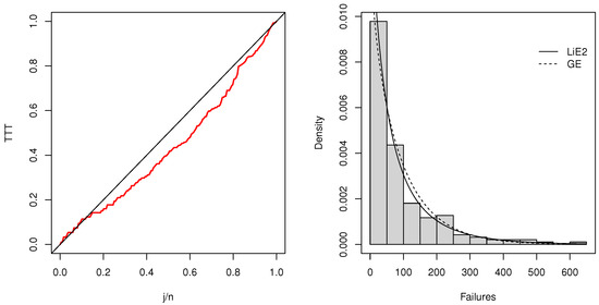
Figure 11. TTT plot of the data set (on the left) and two competing fits for the Failure data (on the right).

For convenience, the data are given Table 5.

Table 5. Data on the successive failures for the air conditioning system of each member in a fleet of 13 Boeing 720 jet air planes.

194	413	90	74	55	23	97	50	359	50	130	487	57	102	15
14	10	57	320	261	51	44	9	254	493	33	18	209	41	58
60	48	56	87	11	102	12	5	14	14	29	37	186	29	104
35	98	54	100	11	181	65	49	12	239	14	18	39	3	12
5	36	79	59	33	246	1	79	3	27	201	84	27	156	21
16	88	130	14	118	44	15	42	106	46	230	26	59	153	104
20	206	5	66	34	29	26	35	5	82	31	118	326	12	54
36	34	18	25	120	31	22	18	216	139	67	310	3	46	210
57	76	14	111	97	62	39	30	7	44	11	63	23	22	23
14	18	13	34	16	18	130	90	163	208	1	24	70	16	101
52	208	95	62	11	191	14	7

The fitting results are given in Table 6. According to the AIC, the LiE2 fit is better than the GE fit. The Kolmogorov–Simirnov test statistic is $0.050017$ with a p-value of $0.7347$. In addition, the EM algorithm gave $\widehat{\lambda }=0.3837683$ and $\widehat{\theta }=0.007553028$, which are close to those obtained from direct maximization.

Table 6. Maximum-likelihood estimates with standard errors in parentheses, log-likelihood and AIC values for failure data.

Model	$\widehat{\mathit{\lambda }}$	$\widehat{\mathit{\theta }}$	$\widehat{\mathit{\alpha }}$	log-lik	AIC
LiE2	0.3800	0.0076		−1033.644	2071.288
	(0.1180)	(0.0014)
GE		0.0102	0.9005	−1036.907	2077.814
		(0.0010)	(0.0852)

9. Conclusions

In this manuscript, we constructed two general probability distribution families using the discrete Lindley distribution. The families contain a baseline distribution which can be manipulated by the user to obtain probability distributions of different shapes. The resulting distributions are not so complex in the sense that the number of parameters of the baseline distribution is increased by one only. As an alternative to the direct maximization of the log-likelihood, we constructed an EM algorithm to compute the ML estimates of the parameters. We mainly focused on the exponential baseline distribution and used the newly defined distributions in real data fitting.

As a part of further research, the introduced distributions may be studied in detail using other simple baseline distributions like Pareto. Also, the Marshall-Olkin approach of construction of bivariate distributions can be used to define the bivariate extensions of the models introduced.

References

- Johnson, N.L.; Kemp, A.W.; Kotz, S. Univariate Discrete Distributions; John Wiley & Sons, Inc.: Hoboken, NJ, USA, 2005. [Google Scholar]
- Hu, X.; Zhang, L.; Sun, W. Risk model based on the first-order integer-valued moving average process with compound Poisson distributed innovations. Scand. Actuar. J. 2018, 5, 412–425. [Google Scholar] [CrossRef]
- Asmussen, S. Ruin Probabilities; World Scientific Publishing: Singapore, 2000. [Google Scholar]
- Klugman, S.; Panjer, H.H.; Willmot, G.E. Loss Models: From Data to Decisions; Wiley: New York, NY, USA, 1998. [Google Scholar]
- Panjer, H.H.; Willmot, G.E. Insurance Risk Models; Society of Actuaries: Schaumburg, IL, USA, 1992. [Google Scholar]
- Nadarajah, S.; Popović, B.V.; Ristić, M.M. Compounding: An R package for computing continuous distributions obtained by compounding a continuous and a discrete distribution. Comput. Stat. 2013, 28, 977–992. [Google Scholar] [CrossRef]
- Gómez-Déniz, E.; Calderín-Ojeda, E. The discrete Lindley distribution: Properties and applications. J. Stat. Comput. Simul. 2011, 81, 1405–1416. [Google Scholar] [CrossRef]
- Abebe, B.; Shanker, R.A. A discrete lindley distribution with applications in biological sciences. Biom. Biostat. Int. J. 2018, 7, 48–52. [Google Scholar] [CrossRef]
- Oliveira, R.P.; Mazucheli, J.; Achcar, J.A. A comparative study between two discrete Lindley distributions. Cienc. Nat. 2017, 39, 539–552. [Google Scholar] [CrossRef][Green Version]
- Tahir, M.H.; Cordeiro, G.M. Compounding of distributions: A survey and new generalized classes. J. Stat. Distrib. Appl. 2016, 3, 13. [Google Scholar] [CrossRef]
- Wolfram Research, Inc. Mathematica, Version 9.0.; Wolfram Research, Inc.: Champaign, IL, USA, 2012. [Google Scholar]
- Nadarajah, S.; Kotz, S. The Exponentiated Type Distributions. Acta Appl. Math. 2006, 92, 97–111. [Google Scholar] [CrossRef]
- Brazauskas, V. Information matrix for Pareto (IV), Burr, and related distributions. Commun. Stat.-Theory Methods 2003, 32, 315–325. [Google Scholar] [CrossRef]
- Cordeiro, G.M.; Brito, R.S. The Beta Power distribution. Braz. J. Probab. Stat. 2012, 26, 88–112. [Google Scholar]
- Gupta, R.D.; Kundu, D. Generalized exponential distributions. Aust. N. Z. J. Stat. 1999, 41, 173–188. [Google Scholar] [CrossRef]
- Nichols, M.D.; Padgett, W.J. A Bootstrap control chart for Weibull percentiles. Qual. Reliab. Eng. Int. 2006, 22, 141–151. [Google Scholar] [CrossRef]
- Lemonte, A.J.; Cordeiro, G.M. The exponentiated generalized inverse Gaussian distribution. Stat. Probab. Lett. 2011, 81, 506–517. [Google Scholar] [CrossRef]
- Barlow, R.E.; Campo, R. Total time on test processes and applications to failure data analysis. In Reliability and Fault Tree Analysis; Barlow, R.E., Fussell, J., Singpurwalla, N.D., Eds.; SIAM: Philadelphia, PA, USA, 1975; pp. 451–481. [Google Scholar]
- Klefsjö, B. TTT-plotting—A tool for both theoretical and practical problems. J. Stat. Plan. Inference 1991, 29, 99–110. [Google Scholar] [CrossRef]
- R Core Team. R: A Language and Environment for Statistical Computing; R Foundation for Statistical Computing: Vienna, Austria, 2020; Available online: https://www.R-project.org/ (accessed on 12 November 2022).
- Proschan, F. Theoretical explanation of observed decreasing failure rate. Technometrics 1963, 5, 375–383. [Google Scholar] [CrossRef]
- Al-Saiary, Z.A.; Bakoban, R.A. The Topp-Leone generalized inverted exponential distribution with real data applications. Entropy 2020, 22, 1144. [Google Scholar] [CrossRef] [PubMed]
Disclaimer/Publisher’s Note: The statements, opinions and data contained in all publications are solely those of the individual author(s) and contributor(s) and not of MDPI and/or the editor(s). MDPI and/or the editor(s) disclaim responsibility for any injury to people or property resulting from any ideas, methods, instructions or products referred to in the content. |
© 2023 by the authors. Licensee MDPI, Basel, Switzerland. This article is an open access article distributed under the terms and conditions of the Creative Commons Attribution (CC BY) license (https://creativecommons.org/licenses/by/4.0/).