Abstract
Source coding maps elements from an information source to a sequence of alphabetic symbols. Then, the source symbols can be recovered exactly from the binary units. In this paper, we derive an approach that includes information variation in the source coding. The approach is more realistic than its standard version. We employ the Shannon entropy for coding the sequences of a source. Our approach is also helpful for short sequences when the central limit theorem does not apply. We rely on a quantifier of the information variation as a source. This quantifier corresponds to the second central moment of a random variable that measures the information content of a source symbol; that is, considering the standard deviation. An interpretation of typical sequences is also provided through this approach. We show how to use a binary memoryless source as an example. In addition, Monte Carlo simulation studies are conducted to evaluate the performance of our approach. We apply this approach to two real datasets related to purity and wheat prices in Brazil.
Keywords:
communication science; discrete memoryless source; entropy; information theory; Monte Carlo simulation; Newton–Raphson method; statistical moments; variance MSC:
28D20
1. Introduction
Entropy is a fundamental concept in science [1,2]. In information theory [3], entropy is the process of coding a discrete memoryless source (DMS) through the first Shannon theorem [4,5]. The law of large numbers was used to prove this theorem [6]. The concept of information theory and its relation to entropy is found in [7]. The reader is referred to [8,9,10] for applications of entropy in statistics to show the relevance of entropy. Two relevant works on statistical mechanics by maximizing entropy were presented in [11,12].
In the entropy context, source coding maps from an information source to a sequence of alphabetic symbols (often using bits). This mapping occurs in such a way that the source symbols may be recovered exactly from the binary units (source coding with no information loss) or recovered within some distortion (source coding with information loss). Such a mapping is the concept behind data compression. Source coding represents symbols of an information source with as few code digits per source symbol as possible [13]. A distributed conditional arithmetic encoding based on source symbol purging has been proposed. Some works devoted to coding finite-length source sequences can be found in [14] and the references therein.
Although various works focus on entropy, they are only associated with the mean (first statistical moment) and not with the variance (second central moment) of the information produced by the source symbols. Information variation (or variability) is an aspect that should be considered in all information analysis. Then, instead of using the entropy as a lower bound on the average letter length of the source coding sequences, one can adopt an interval based on information variation according to a confidence level stated by the code designer. Nevertheless, a point estimate is often considered rather than an interval estimate. To estimate the entropy of symbol sequences, an excellent reference is [15].
To the best of our knowledge, there are no published studies dealing with DMS in a general context, independent of the probabilistic model that generates the data. Only one unpublished work on the Shannon entropy of sequences exists, in which a plugin estimator was proposed in 2018 by the authors of this paper [16]. Then, in another unpublished work in 2021 [17], the estimation of the variance of the Shannon entropy was stated. This work utilized a plugin estimator for the variance and provided asymptotic properties of the estimator over the conditions of a probabilistic simplex model. The study presented in [17] is different from that proposed earlier in [16] and formalized in the present investigation because we do not fix a probabilistic model but look at sequence-based empirical properties and not at the model. In [17], the asymptotic properties of the plugin estimator are verified. In the present study, we use the variance of the plugin estimator and the entropy estimator to characterize the DMS. For example, we can determine with a high degree of confidence whether the source is degenerate or it generates low or high entropy, which, in practical terms, helps us to determine if the sequence is predictable or not. In an old study presented in 1974 [18], some moments of an estimate of the Shannon measure of information were introduced for the multinomial distribution. In that work, a resampling mechanism was employed to directly evaluate the plugin estimator’s variability and verify what entropy estimator would be most appropriate in an ergodic environment based on the multinomial distribution. Therefore, the proposal introduced in [18] is based on a multinomial probabilistic model and not a general framework such as we state in the present investigation.
A work presented in 2008 [19] proposed an estimation of the entropy of binary time series. In that work, an estimator of the variance was provided via bootstrapping and did not utilize a plugin method. In [19], the authors were not interested in the variation directly as a classification mechanism, but the variation was employed to assess the Shannon estimator’s behavior calculating the bias and variance via bootstrapping.
Therefore, the primary objective of our investigation is to develop a method that includes information variation in the source coding. We use a quantifier of information variation as a source. This quantifier is related to the second central moment of a random variable that measures the information content of a source symbol—that is, through the variance and its corresponding standard deviation. Our approach is also helpful for short sequences in which the central limit theorem does not have enough support to be applied. Based on our approach, we also provide an interpretation of typical sequences. Note that the relevance of describing information variation lies in improving predictability by considering the inherent variability of the source, which is often not considered. Therefore, our proposal gives an improvement in the source coding performance because although the literature provides several Shannon measures, it does not usually consider the variability of DMS. If this variability is high, then such Shannon measures have low predictability.
The rest of the paper is organized as follows. Section 2 introduces the proposed approach for information variation in sources of coding sequences. In Section 3, we state an evaluation of entropy for finite sequences. In Section 4, an estimation strategy for atypical sequences is developed. Section 5 presents an illustration that uses binary DMS, in which the output is zero with a probability or one with its complement. In Section 6, we evaluate the proposed approach with Monte Carlo simulation studies. In Section 7, empirical applications of our proposal are provided. Concluding remarks are established in Section 8.
2. Variation of Information
Consider a DMS represented by a random variable U that accepts symbols from a finite alphabet, that is, the sequence stated as
with probability of occurrence at a time instant, l namely, denoted by , for , where
The stationary distribution for the DMS model defined in (2) is independent over time, that is, , for all . In addition, for each symbol produced, the associated amount of information is given by
with being defined in (1). For simplicity, let us refer to established in (3) as .
A smooth functional of the probability distribution of the source (first moment) is recognized as the Shannon entropy of the DMS [20] and formulated as
where is the expected value operator and is the information amount of U defined in (3), with being a random variable.
We propose to use information variation as a compound of a functional based on the second moment of the probability distribution of the source established as
where is the variance operator. One can prove that by the Jensen inequality. Therefore, the variation can be computed employing
with the expression stated in (6) being obtained by applying to (4) the multiplication rule for series, also called the Lagrange identity, which allows us to attain at
Therefore, by using (5) and (7), after a simple algebra, we reach the formula given in (6).
Definition 1 (Degenerated sources).
We define two types of degenerated sources as follows:
- (i)
- [Type I source] This is denoted by and associated with the sequence , for , where there exists , such that and , for all .
- (ii)
- [Type II source] This is denoted by and related to the sequence , for , where , for all and , with denoting the cardinality of a set.
Proposition 1.
The variation of information is null if and only if the source is degenerated; that is, , for any or
Proof.
(⇐) follows directly from , for all k, and , for all . Regarding the formula stated in (6), for type II sources, there are identical terms in the first summation and terms in the second summation. Therefore, we have that
(⇒) Without loss of generality, consider the case where is sorted in descending order; that is, . This means that because the terms do not count. Thus, the possible solutions are of the type , for and , for all . Note that two trivial solutions are the following:
- and , for , with .
- , for , with .
Therefore, this concludes the proof. □
It is worth noting that the sources denoted by and in Definition 1 are two particular types of degenerated distributed DMS. The first type has just one symbol with nonzero probability, so it always sends the same symbol with probability one. The second type is a uniformly distributed source, which is often a limiting case. Although -sources are a subset of -sources (by assuming ), we distinguish them as distinct types of sources.
3. Evaluation of Entropy for Finite Sequences
Let be a sequence of observed counts of alphabetical symbols in a DMS sample of size L. We define the sample relative frequency of the k-th symbol employing
where is the number of symbols in the sample.
The most common manner of estimating defined in (4) is nonparametrically using the plugin estimator provided as
where is given in (8) and K is the length of the sequence. Note that the estimate stated in (9) has been a subject of much research for decades [21,22,23,24,25]. Based on (5), we propose to use a statistic as a plugin estimator of information variation formulated as
We can prove that the estimators and defined in (9) and (10) are consistent and asymptotically unbiased for and , respectively. These desirable statistical properties can be proved by using a Taylor expansion of the functions and about the point and confining ourselves to derivatives of fourth order.
Consider a DMS sample of size L. Then, based on the central limit theorem, as , we have that , that is, converges in distribution to , where . Thus, we obtain that
where ∼ and , as usual in statistics, mean “distributed exactly as” and “approximately (or asymptotically) distributed as”, respectively.
If the condition does not hold to apply the central limit theorem, as also usual in statistics, we can consider the assumption established as
In addition, as is an estimator of the information variation [22], we may state that
where is the chi-square distribution with degrees of freedom.
Consequently, from the result presented in (12), we get
Hence, based on the expressions given in (13) and (14), we obtain
where is the Student-t distribution with degrees of freedom. Naturally, for short sequences, it is more appropriate to use the Student-t statistic defined in (15). Thus, a confidence bound for is expressed as
where is the upper -th percentile of the Student-t distribution with degrees of freedom [26]. Note that, for large L, based on the asymptotic distribution reached in (11), or for small L, considering the assumption established in (14), in the case of a known variance , and the theory stated in [26], we can calculate a confidence bound for by means of
where is the upper -th percentile of the standard normal distribution, which is the inverse of the cumulative distribution function .
If one sets a confidence level at, say , then, for sequence outcomes of the source (all with small length L), the sample entropy value should not exceed the bound given in (16) in of cases; or the bound given in (17) in of cases, if L is large. As a result, rather than the fundamental limit of , which can be reached asymptotically as the length of the source sequences increases indefinitely, we can expect to code the output with bits per source symbol.
The efficiency of a source coding run for a specific given sequence is determined by using a conventional expression that is defined as
where is the average number of bits per source letter. Instead of adopting the conventional formula stated in (18), we propose to assess such an efficiency (especially in the cases of short sequences and high entropy variability DMS) at a confidence level of , according to
4. Atypical Sequences
Let us now shift the focus to long sequences. In this scenario, a statistical interpretation for atypical sequences can be formulated.
All sequences generated from the source that result in a sample entropy are considered typical if any of them fall within a confidence interval indicated as
Definition 2 (-atypical sequence).
Let be an arbitrary value. For any sequence (a source sample) with a length L of symbols, the sample entropy is called an ε-atypical sequence if it is outside the range
The following question arises. What is the confidence level at which the confidence interval given in (19) for the entropy coincides with the interval stated in Definition 2 through the expression given in (20)? To respond to this question, we must impose the relationship formulated as
In the case of the expression given in (21), the confidence level is interpreted as the probability of an atypical sequence occurring; that is, . Therefore, we have that
Typical sequences (in the sense that the sample entropy is -closed to the source’s entropy) constitute virtually 100% of the sequences if the sequence length L is sufficiently large.
Another key concept in information theory is the asymptotic equipartition property. The extension of the source U considers L-grams as the new symbols. This has an alphabet , with probabilities , for . Note that, although we have
it is possible to show that -typical sequences hold [27] with the interval stated as
Therefore, from the formula given in (22), we get the set of typical sequences formulated as
It is worth noting that the expression given in (23) is constant for all , with
By the definition of degenerated sources stated in Definition 1, we see that large extensions of a DMS become type II asymptotically degenerated. The entropy becomes exactly with no information variation.
5. Illustrative Example
As an illustration, consider the following example. Assume a binary DMS with an output of zero with a probability of p or one with a probability of . For this case, the quantifiers given in (4) and (5) simplify, respectively, to two expressions stated as
The binary entropy has a well-known shape [20]. We sketch and defined in (24) and (25) over p in Figure 1.
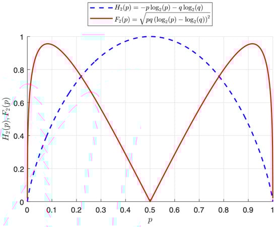
Figure 1.
Plots of and on p.
Regarding p, there are five values worth mentioning. Consider the ordered set of values stated as
where and defined in (26) are points at which the function reaches a maximum. We can see in Figure 1 that and . From this figure, note that three limit cases have no variance (binary degenerated sources): (i) , (ii) (in both cases, the source transmits just the same symbol and has null entropy), and (iii) . Surprisingly, in this last case (iii), with equiprobable sequences and maximum entropy, there is no variance in the amount of information.
Observe that, whatever the length of the sequence of source symbols, the average information per source letter is equal to the entropy. However, the points of maximum variability in the information content seem less, which is well known in the literature.
We begin by looking into the behavior of stated as
A plot of the derivative of defined in (27) is shown in Figure 2. Note that the three points in this figure have infinite derivative values (singular points), which correspond to the three limit cases mentioned earlier in (i)–(iii). From the expression stated in (27), we define a function formulated as
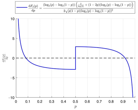
Figure 2.
Plot of the derivative of the binary variation over p.
Notice that the two critical points (stationary values) of occur when . In Figure 3, we can observe the plot of the function g defined in (28).

Figure 3.
Plot of the function g over p and its two roots.
The Newton-Raphson (NR) algorithm was applied to approximate the two roots of g defined in (28). With a tolerance of and four iterations, the values (with an initial value to start the algorithm equal to 0.1) and (with an initial value equal to 0.9) were obtained. The value of the derivative is around 0.956137 at the two maximum points, that is, . In addition, we calculate the intersection points of the two curves of Figure 1, where . In the range between the two points, the standard deviation of the entropy is less than the entropy itself. We use this range to characterize the binary DMS with low entropy variability.
By using the coefficient of variation (CV) as described in [26,28], we consider the formula defined as
We plot the CV stated in (29) through Figure 4. From the expression formulated in (29), we reach the function given by
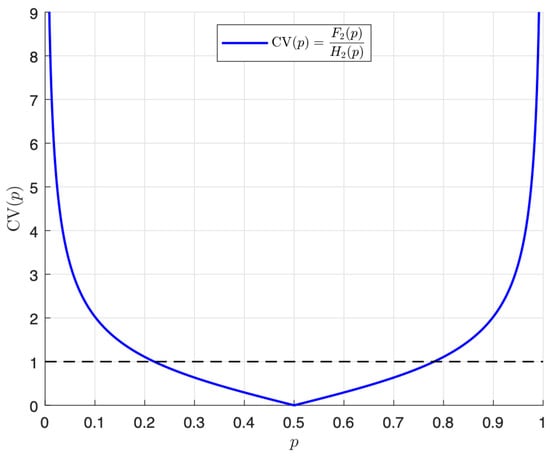
Figure 4.
Plot of the coefficient of variation of the entropy.
Figure 5 shows the plot of the function D expressed in (30) over p. Let and be the roots of the function D, with . Again, the NR algorithm is used, and after three iterations and a tolerance of , the values (with an initial value to start the algorithm equal to 0.3) and (with an initial value equal to 0.7) were obtained.
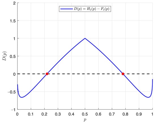
Figure 5.
Plot of the function D over p and its two roots.
The following definition is derived from analyzing the behavior of the CV over p as expressed in (29).
Definition 3 (Low entropy variability DMS).
A binary DMS that takes the values zero with a probability p, and one with a probability , associated with the function D defined in (30) whose roots are and , is called a low-entropy variability DMS if and only if we have
6. Monte Carlo Simulation Studies
To illustrate the previous results, we consider a binary source U generated by a Bernoulli process (sequence of identically independent distributed random variables). Assume that we run a Bernoulli trial every second, for t seconds, with and , and the value equal to one being the arrival of a bit, for example.
We use Monte Carlo simulation to assess the distributional behavior of and , as given in expressions stated in (14) and (15), respectively. The number of Monte Carlo replications equals . The time is in seconds, and we set only by symmetry.
The kernel density estimates of applied to are shown in Figure 6. By visual inspection, we observe that the kernel density estimate of the distribution of shows evidence of a good approximation to the standard normal distribution (symmetric around to mean equal to zero, tails are decaying to zero, and turning points around of and 1).
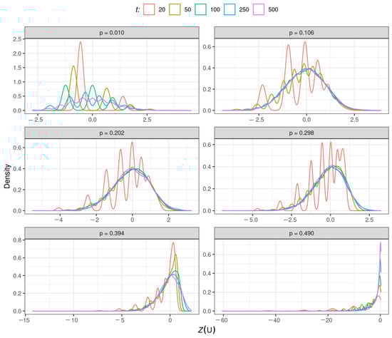
Figure 6.
Kernel density estimates of the statistic for the indicated value of p and t.
We observe that the approximation to the standard normal distribution is poor for short periods (), considering all values of p as expected (the law of large numbers requires observing the source for a sufficiently large period). When p is close to 0 or 0.5, the source tends to degenerate, and the approximation of the standard normal distribution of is more challenging to achieve.
Normality of the distribution given in (14) was also checked through the Kolmogorov-Smirnov (KS) test [29]. Table 1 contains the proportion of times that the KS test rejects the null hypothesis of normality. We use a 5% significance level, and then about 5% of these tests should reject the null hypothesis. As expected, the results generally show strong acceptance of the null hypothesis. However, the type I error is inflated for short periods of observation of the source, or p tending to 0.5.

Table 1.
Null rejection rates of the KS test to detect goodness of fit for the normal distribution approximation of with the indicated values of t and p.
We also compute the coverage probability (CP) of a 95% confidence bound based on the results stated in (17). The CP is computed as
where is an indicator function such that belongs to the r-th bound , with being the r-th upper limit estimates of the 95% confidence bound defined in (17). Table 2 reports empirical values for the CP defined in (31). From the results in this table, we conclude that the CP approaches the 95% nominal level as the sample size increases, as expected. For example, for and , the CP is 93%, and for and , the CP is 95%.
Table 2.
A CP of a 95% confidence bound for the normal distribution approximation of with the indicated value of p and t.
Figure 7 depicts the kernel estimates of the distribution of across t and p. The boxplot of is displayed in each panel. All densities look roughly with the Student-t distribution (symmetric around zero and fast decay of tails to zero when t is large by the convergence of the Student-t distribution to the normal one). Note that, in each panel, as t increases, the fluctuations of the source stabilize around a value that depends only on p. Then the information of provides a scale correction of the statistic given in (15), as expected by the law of large numbers. In short periods, is more stable than , as expected. The KS test with the Student-t distribution as a reference confirms these conjectures.
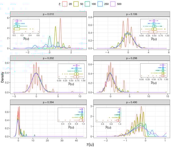
Figure 7.
Kernel density estimates of the statistic for the indicated value of p and t.
Table 3 contains the proportion of times that the KS test rejects the null hypothesis of a Student-t distribution. We use a 5% significance level. The type I error is also inflated for short-time observation () of the source, and p close to 0 or 0.5. As expected, the results generally agree with the null hypothesis.
Table 3.
Null rejection rates of the KS test to detect goodness of fit for the Student-t distribution with degrees of freedom with the indicated values of t and p.
Table 4 reports empirical values for the CP defined in (31) changing the limit by stated in (16). From the results in this table, we conclude that the CP approaches the 95% nominal level as the sample size increases, as expected. For example, for and , the CP is 94%, and for and , the CP is 92%.
Table 4.
A CP of a 95% confidence bound for the Student-t distribution with degrees of freedom of for the indicated value of p and t.
7. Empirical Applications
The first application with real data is related to purity of information. To show the use of information variation, we consider the Iris dataset obtained from [30], which is widely used in pattern recognition. This set can be considered a DMS with three prior symbols (), each with 50 observations and a total of instances. The symbols correspond to three species of iris plants: setosa (symbol 1), virginica (symbol 2), and versicolor (symbol 3). For each species, the variables are petal length (PL), petal width (PW), sepal length (SL), and sepal width (SW). The Shannon entropy given in (9) provides a measure of information purity. We take subsets of the Iris data containing only one species. We are interested in identifying how pure each species is, and we assume that the source includes information variation when collecting the data. Because we do not know the true probability distribution of the source, we need to employ the plugin estimators defined in (9) and (10). We intuitively know that we have 100% knowledge of the Iris species because we have only a single species selected. As a result, we must be at the lower bound of entropy without information variation, which means that for each species, we have and respectively. Then, we have complete knowledge of the contents of each set. If we ask to draw one observation at random and predict the species based only on the location of each species, for example, of Iris virginica species, we know that a kind of Iris virginica will be sketched. Nonetheless, in the Iris dataset, we have three species of iris, each representing 1/3 of the dataset. Thus, we expect a high entropy if we include the complete data. If we imagine an urn filled with different-colored balls representing the species of iris, we have less knowledge about what color of the ball (what species) we would draw randomly from the urn. In this case, and
A second application with real data is associated with wheat prices in Brazil, whose daily time series is available at www.cepea.esalq.usp.br/br/indicador/milho.aspx, accessed on 1 January 2022. The data were observed from 2 February 2002 to 25 October 2019. First, we subtract the original series to get stationarity. The series is flat, oscillating about a mean above zero, and the autocorrelation trails off as one might expect for a stationary series (see Figure 8). Now, we construct a new series of symbols +1 and −1 for detecting changes in prices for the differentiated series, such as in a nonparametric run test [31]. The new series can be considered a binary source that reflects whether the series of differences assumes positive (: price increase) or negative (: price decrease) values from wheat prices in Brazil. We compute the Shannon and information variation measures, getting and . As our source is binary, we note that the entropy estimate is close to one, indicating that increasing or decreasing prices are practically equiprobable.
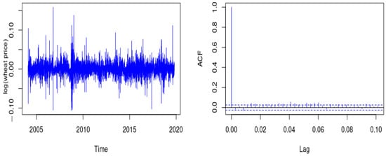
Figure 8.
Log wheat prices after deleting weekly and seasonal cycles (left) and ACF plot (right).
Because the observation time is relatively long (), we can utilize the approximation given in (19). In this way, if we consider a confidence level of 95%, we obtain the interval (0.918; 0.922) for the Shannon entropy. The result indicates that, with 95% confidence, our series is typical and . This result suggests that it is challenging to predict and detect changes in wheat prices in Brazil so that other methods should be studied. Note that this is simply an illustrative example to show how our new methodology can be used. We do not intend to solve a new problem with our methodology for now. Ideas about cryptography, cryptocompression, and cryptocurrencies, as well as other possible applications, are proposed in the conclusions of the present article related to future research.
8. Concluding Remarks
In this paper, we have proposed and derived a novel approach that includes information variation in the source coding. This approach is more realistic than its standard version. We have employed the Shannon entropy for coding sequences of a source. In addition, the new approach is helpful for short sequences in which the central limit theorem does not have enough support to be applied. We employed a quantifier of information variation for a source related to the variance of the information content of a source symbol. Introducing a new parameter for a discrete memoryless source, namely the information variation, seems to be as essential as the concept of entropy itself. For short sequences, it is not the source’s entropy that should be used to calculate the efficiency of source coders, but rather the sample entropy. In addition to proposing the calculation of a more realistic estimate for the entropy, now depending on the sequence length from the source, a naive and didactic interpretation of typical sequences was presented. We introduced illustrations by assuming a binary discrete memoryless source, in which the output was either zero with a certain probability or one with its complementary probability. In addition, Monte Carlo simulation studies were conducted to evaluate the performance of our approach, providing evidence of the adequate performance of our proposal. Moreover, we have applied our approach to two real datasets related to purity and wheat prices in Brazil.
Potential further applications of our proposal are in assessing the randomness of sequences. Some open questions from the present investigation remain. Is there always a maximum variation in the sample entropy for some particular (nonbinary) probability assignment? The answer needs further developments that we leave for future work. In addition, the usage of other types of estimation methods; statistical moments—robust statistical methods and entropy configurations and sequences, as well as different types of inequalities [32,33,34,35,36,37]—will be considered, and we hope to report their findings in future publications. Similarly, as we have assumed statistical independence in our proposal, the extension to dependent sequences is a good topic for future extension. Moreover, traditional autoregressive models and a copula-based Markov chain are now available to be further considered [38]. We suggest investigating the possibility of incorporating a nonparametric estimation of the Shanon diversity index into our proposal [39]. In this way, we can obtain a reasonable confidence level when bias is suspected in the sample.
Our work may be of particular interest to specialists in the field of cryptography in solving digital security problems [40]. Coding methods and their application in information security systems, cryptocompression systems, and data compression are relevant topics to be considered [10,41]. For example, the application of arithmetic coding methods in cryptographic information protection systems is considered in [42]. Volatile time series and information flow analyses based on cryptocurrency data have been studied in [43]. A new approach to predicting cryptocurrency is stated in [44]. These frameworks open new avenues to apply the results obtained in the present research.
Author Contributions
Conceptualization, H.M.d.O. and R.O.; Data curation, H.M.d.O., R.O. and C.M.-B.; Formal analysis, H.M.d.O., R.O., C.M.-B., V.L. and C.C. Investigation, H.M.d.O., R.O., C.M.-B., V.L. and C.C. Methodology, H.M.d.O., R.O., C.M.-B., V.L. and C.C. Writing—original draft, H.M.d.O., R.O., C.M.-B. and C.C. Writing—review and editing, V.L. All authors have read and agreed to this version of the manuscript.
Funding
This research was partially supported by the National Council for Scientific and Technological Development (CNPq) through the grant 305305/2019-0 (R.O.), and Comissão de Aperfeiçoamento de Pessoal do Nível Superior (CAPES), from the Brazilian government; and by FONDECYT, grant number 1200525 (V.L.), from the National Agency for Research and Development (ANID) of the Chilean government under the Ministry of Science and Technology, Knowledge, and Innovation.
Institutional Review Board Statement
Not applicable.
Informed Consent Statement
Not applicable.
Data Availability Statement
The data and computational codes are available upon request.
Conflicts of Interest
The authors declare no conflict of interest.
Abbreviations
Next, we present the abbreviations considered in this work to facilitate its reading:
| ACF | Auto-correlation function |
| CV | Coefficient of variation |
| DMS | Discrete memoryless source |
| CP | Coverage probability |
| KS | Kolmogorov-Smirnov |
| NR | Newton-Raphson |
| PL | Petal length |
| PW | Petal width |
| SL | Sepal length |
| SW | Sepal width |
References
- Ben-Naim, A. A Farewell to Entropy: Statistical Thermodynamics Based on Information; World Scientific: New York, NY, USA, 2008. [Google Scholar]
- Kafri, O.; Kafri, H. Entropy: God’s Dice Game; CreateSpace Independent Publishing Platform: Scotts Valley, CA, USA, 2013. [Google Scholar]
- Tsalatsanis, A.; Hozo, I.; Djulbegovic, B. Research synthesis of information theory measures of uncertainty: Meta-analysis of entropy and mutual information of diagnostic tests. J. Eval. Clin. Pract. 2021, 27, 246–255. [Google Scholar] [CrossRef] [PubMed]
- Shannon, C.E. A mathematical theory of communication. Bell Syst. Tech. J. 1948, 2, 623–656. [Google Scholar] [CrossRef]
- Nikooravesh, Z. Estimation of the probability function under special moments conditions using the maximum Shannon and Tsallis entropies. Chil. J. Stat. 2018, 9, 55–64. [Google Scholar]
- Fierro, R.; Leiva, V.; Moeller, L. The Hawkes process with different exciting functions and its asymptotic behavior. J. Appl. Probab. 2015, 52, 37–54. [Google Scholar] [CrossRef]
- Ellerman, D. New Foundations for Information Theory: Logical Entropy and Shannon Entropy; Springer: New York, NY, USA, 2021. [Google Scholar]
- Alonso, A.; Molenberghs, G. Evaluating time to cancer recurrence as a surrogate marker for survival from an information theory perspective. Stat. Methods Med. Res. 2008, 17, 497–504. [Google Scholar] [CrossRef] [PubMed]
- Kowalski, A.M.; Portesi, M.; Vampa, V.; Losada, M.; Holik, F. Entropy-based informational study of the COVID-19 series of data. Mathematics 2022, 10, 4590. [Google Scholar] [CrossRef]
- Iatan, I.; Drǎgan, M.; Dedu, S.; Preda, V. Using probabilistic models for data compression. Mathematics 2022, 10, 3847. [Google Scholar] [CrossRef]
- Jaynes, E.T. Information theory and statistical mechanics. Phys. Rev. 1957, 106, 620–630. [Google Scholar] [CrossRef]
- Jaynes, E.T. Information theory and statistical mechanics II. Phys. Rev. 1957, 108, 171–190. [Google Scholar] [CrossRef]
- Gray, R.M. Source Coding Theory; Springer: New York, NY, USA, 2012. [Google Scholar]
- Barron, A.R.; Rissanen, J.; Yu, B. The minimum description length principle in coding and modeling. IEEE Trans. Inf. Theory 1998, 44, 2743–2760. [Google Scholar] [CrossRef]
- Schürmann, T.; Grassberger, P. Entropy estimation of symbol sequences. Chaos 1996, 6, 414–427. [Google Scholar] [CrossRef] [PubMed]
- de Oliveira, H.M.; Ospina, R. A note on the Shannon entropy of short sequences. arXiv 2018, arXiv:1807.02603. [Google Scholar]
- Ricci, L.; Perinelli, A.; Castelluzzo, M. Estimating the variance of Shannon entropy. arXiv 2021, arXiv:2105.12829. [Google Scholar] [CrossRef] [PubMed]
- Hutcheson, K.; Shenton, L.R. Some moments of an estimate of Shannon’s measure of information. Commun. Stat. Theory Methods 1974, 2, 89–94. [Google Scholar] [CrossRef]
- Gao, Y.; Kontoyiannis, I.; Bienenstock, E. Estimating the entropy of binary time series: Methodology, some theory and a simulation study. Entropy 2008, 10, 71–99. [Google Scholar] [CrossRef]
- Gallager, R.G. Information Theory and Reliable Communication; Wiley: New York, NY, USA, 1968. [Google Scholar]
- Miller, G. Note on the bias of information estimates. In Information Theory in Psychology; Free Press: Glencoe, UK, 1955; pp. 95–100. [Google Scholar]
- Basharin, G. On a statistical estimate for the entropy of a sequence of independent random variables. Theory Probab. Its Appl. 1959, 4, 333–336. [Google Scholar] [CrossRef]
- Antos, A.; Kontoyiannis, I. Convergence properties of functional estimates for discrete distributions. Random Struct. Algorithms 2001, 19, 163–193. [Google Scholar] [CrossRef]
- Paninski, L. Estimation of entropy and mutual information. Neural Comput. 2003, 15, 1191–1253. [Google Scholar] [CrossRef]
- Zhang, Z. Asymptotic normality of an entropy estimator with exponentially decaying bias. IEEE Trans. Inf. Theory 2013, 59, 504–508. [Google Scholar] [CrossRef]
- Montgomery, D.C.; Runger, G.C. Applied Statistics and Probability for Engineers; Wiley: New York, NY, USA, 2010. [Google Scholar]
- Cover, T.M.; Thomas, J.A. Elements of Information Theory; Wiley: New York, NY, USA, 2012. [Google Scholar]
- Riquelme, M.; Leiva, V.; Galea, M.; Sanhueza, A. Influence diagnostics on the coefficient of variation of elliptically contoured distributions. J. Appl. Stat. 2011, 38, 513–532. [Google Scholar] [CrossRef]
- Razali, N.; Wah, Y. Others power comparisons of Shapiro-Wilk, Kolmogorov-Smirnov, Lilliefors and Anderson-Darling tests. J. Stat. Model. Anal. 2011, 2, 21–33. [Google Scholar]
- Anderson, E. The irises of the Gaspe Peninsula. Bull. Am. Iris Soc. 1935, 59, 2–5. [Google Scholar]
- Gibbons, J.; Chakraborti, S. Nonparametric Statistical Inference; CRC Press: Boca Raton, FL, USA, 2014. [Google Scholar]
- Athayde, E.; Azevedo, A.; Barros, M.; Leiva, V. Failure rate of Birnbaum-Saunders distributions: Shape, change-point, estimation and robustness. Braz. J. Probab. Stat. 2019, 33, 301–328. [Google Scholar] [CrossRef]
- Velasco, H.; Laniado, H.; Toro, M.; Leiva, V.; Lio, Y. Robust three-step regression based on comedian and its performance in cell-wise and case-wise outliers. Mathematics 2020, 8, 1259. [Google Scholar] [CrossRef]
- Lillo, C.; Leiva, V.; Nicolis, O.; Aykroyd, R.G. L-moments of the Birnbaum-Saunders distribution and its extreme value version: Estimation, goodness of fit and application to earthquake data. J. Appl. Stat. 2018, 45, 187–209. [Google Scholar] [CrossRef]
- Balakrishnan, N.; Leiva, V.; Sanhueza, A.; Cabrera, E. Mixture inverse Gaussian distribution and its transformations, moments and applications. Statistics 2009, 43, 91–104. [Google Scholar] [CrossRef]
- Santos-Neto, M.; Cysneiros, F.J.A.; Leiva, V.; Barros, M. On a reparameterized Birnbaum-Saunders distribution and its moments, estimation and applications. Revstat Stat. J. 2014, 12, 247–272. [Google Scholar]
- Alomari, M.W.; Chesneau, C.; Leiva, V. Grüss-type inequalities for vector-valued functions. Mathematics 2022, 10, 1535. [Google Scholar] [CrossRef]
- Sun, L.H.; Huang, X.W.; Alqawba, M.S.; Kim, J.M.; Emura, T. Copula-Based Markov Models for Time Series: Parametric Inference and Process Control; Springer: New York, NY, USA, 2020. [Google Scholar]
- Chao, A.; Shen, T.J. Nonparametric estimation of Shannon’s index of diversity when there are unseen species in sample. Environ. Ecol. Stat. 2003, 10, 429–443. [Google Scholar] [CrossRef]
- Ogut, H. The configuration and detection strategies for information security systems. Comput. Math. Appl. 2013, 65, 1234–1253. [Google Scholar] [CrossRef]
- Barannik, V.; Sidchenko, S.; Barannik, N.; Barannik, V. Development of the method for encoding service data in crypto-compression image representation systems. East.-Eur. J. Enterp. Technol. 2021, 3, 111. [Google Scholar]
- Havrylov, D.; Shaigas, O.; Stetsenko, O.; Babenko, Y.; Yroshenko, V. Application of arithmetic coding methods in cryptographic information protection systems. In Proceedings of the CEUR Workshop in Cybersecurity Providing in Information and Telecommunication Systems, Kyiv, Ukraine, 26 October 2021; pp. 125–136. Available online: ceur-ws.org (accessed on 1 January 2023).
- Sheraz, M.; Dedu, S.; Preda, V. Volatility dynamics of non-linear volatile time series and analysis of information flow: Evidence from cryptocurrency data. Entropy 2022, 24, 1410. [Google Scholar] [CrossRef]
- Mahdi, E.; Leiva, V.; Mara’Beh, S.; Martin-Barreiro, C. A new approach to predicting cryptocurrency returns based on the gold prices with support vector machines during the COVID-19 pandemic using sensor-related data. Sensors 2021, 21, 6319. [Google Scholar] [CrossRef] [PubMed]
Disclaimer/Publisher’s Note: The statements, opinions and data contained in all publications are solely those of the individual author(s) and contributor(s) and not of MDPI and/or the editor(s). MDPI and/or the editor(s) disclaim responsibility for any injury to people or property resulting from any ideas, methods, instructions or products referred to in the content. |
© 2023 by the authors. Licensee MDPI, Basel, Switzerland. This article is an open access article distributed under the terms and conditions of the Creative Commons Attribution (CC BY) license (https://creativecommons.org/licenses/by/4.0/).