Abstract
Learning density estimation is important in probabilistic modeling and reasoning with uncertainty. Since B-spline basis functions are piecewise polynomials with local support, density estimation with B-splines shows its advantages when intensive numerical computations are involved in the subsequent applications. To obtain an optimal local density estimation with B-splines, we need to select the bandwidth (i.e., the distance of two adjacent knots) for uniform B-splines. However, the selection of bandwidth is challenging, and the computation is costly. On the other hand, nonuniform B-splines can improve on the approximation capability of uniform B-splines. Based on this observation, we perform density estimation with nonuniform B-splines. By introducing the error indicator attached to each interval, we propose an adaptive strategy to generate the nonuniform knot vector. The error indicator is an approximation of the information entropy locally, which is closely related to the number of kernels when we construct the nonuniform estimator. The numerical experiments show that, compared with the uniform B-spline, the local density estimation with nonuniform B-splines not only achieves better estimation results but also effectively alleviates the overfitting phenomenon caused by the uniform B-splines. The comparison with the existing estimation procedures, including the state-of-the-art kernel estimators, demonstrates the accuracy of our new method.
MSC:
62G05
1. Introduction
Nonparametric density estimation avoids the parametric assumptions in probabilistic modeling and reasoning, which achieves flexibility in data modeling while reducing the risk of model misspecification [1,2]. Hence, nonparametric density estimation is an important research area in statistics. In this paper, we focus on the estimation of univariate density functions, which is a classic problem in nonparametric statistics. We perform density estimation with nonuniform B-splines. By introducing the error indicator attached to each interval for density estimation, we propose an adaptive strategy to generate a nonuniform knot vector.
There are four main techniques for nonparametric estimation, i.e., histograms, orthogonal series, kernels, and splines. Histograms transform the continuous data into discrete data, while important information may be lost during the discretization process [3]. Kernel density estimation is one of the most famous methods for density estimation, which still remains an active research area (see [4] and references therein). In addition to kernel density estimators, orthogonal series estimators are also widely used, e.g., [5,6,7,8]. Terrell and Scott investigated some of the possibilities for the improvement of univariate and multivariate kernel density estimates by varying the window over the domain of estimation, pointwise and globally [9]. However, the global nature of orthogonal series estimators limits their applications.
Since B-spline basis functions possess the property of local support, local density estimators based on uniform B-splines have been discussed in [10,11,12,13]. In addition to the local support property, B-spline basis functions are also piecewise polynomials, which demonstrates their advantages where intensive numerical computations have been conducted after estimation [13,14,15]. In addition, local density estimators based on different splines have also been studied, e.g., logsplines [16,17], smoothing splines [18], penalized B-splines [19], and shape-constrained splines [20]. Recently, a Galerkin method was introduced to compute a B-spline estimator [21].
The important part of any basis estimation procedure is the bandwidth selection method. The existing literature on bandwidth is quite rich (see [21,22,23,24,25] and references therein). It should be noted that the least squares cross-validation (LSCV) formula in closed form was proposed in [21], which can be used to determine the bandwidth efficiently.
In this paper, we use nonuniform B-splines as density estimators. By introducing the local error indicator attached to the interval, we design an adaptive refinement strategy, which increases the approximation capability of the local density estimator. The numerical experiments show that our adaptive local density estimation produces a smaller approximation error than that with uniform B-splines. Comparison with the state-of-the-art density estimation methods shows that our adaptive method can approximate data with a comparable squared error and a significantly smaller absolute error than other kernel density estimators.
The remainder of the paper is organized as follows. The next section reviews the definition of B-spline basis functions and their corresponding piecewise polynomial space. In Section 3, we detail the proposed method for density estimation based on B-splines. In Section 4, we propose an adaptive knot refinement strategy. Numerical experiments are provided in Section 5. Finally, Section 6 ends with conclusions.
2. B-Splines
Given a knot vector , where and , the B-spline basis functions of degree k (order ) are defined in a recursive fashion [26]:
The B-spline basis functions are nonnegative and have local support (i.e., is a nonzero polynomial on ). In addition, the B-spline basis functions form a partition of unity for [27]. Figure 1 shows the cubic and quadratic B-spline basis functions defined in .
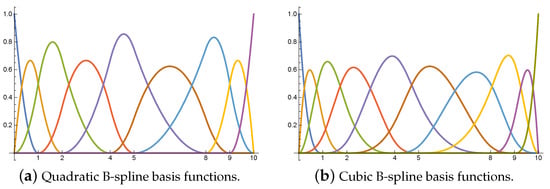
Figure 1.
B-spline basis functions defined in the interval . (a) Knot vector . (b) Knot vector .
A B-spline of degree k is defined [28] as
where is the i-th control coefficient, and is the i-th B-spline basis function, which is defined based on the knot vector . A B-spline whose knot vector is evenly spaced is known as a uniform B-spline. Otherwise, the B-spline is called a nonuniform B-spline.
Let be a sequence of distinct real numbers
where ,
which forms a partition of the interval . The space of piecewise polynomials of degree k with smoothness over the partition is defined by
where is the space of all the polynomials of degree k, and is the space consisting of all the functions that are continuous at with order .
Lemma 1
([29]). Given the knot vector U, the set of B-spline basis functions defined as (1) forms an alternative basis for the piecewise polynomial space .
Moreover, the approximation capabilities of to a sufficiently smooth function defined over were described in [30]. It was shown that a sufficiently smooth function can be approximated with good accuracy by B-splines.
3. Density Estimation with B-Splines
Let be an independent identically distributed random sample from a continuous probability density function f, . Zong proposed a method to find B-spline estimates of a one-dimensional and two-dimensional probability density function from a sample [31].
We define an estimate of in the form:
where are coefficients. To fix the estimate in the form of B-splines, we need to specify the degree k, the basis functions , and the coefficients .
3.1. Selecting the Degree and the Knot Vector
The degree k and the knot vector U need to be specified a priori to determine the basis functions. Based on the approximation ability and flexibility of the quadratic and cubic B-splines, quadratic or cubic B-splines are usually chosen for local density estimation [21,31,32]. The selection of the knot vector is challenging and time consuming. Even when we restrict the knot vector to a uniform case, we still need to specify:
- (1)
- and (i.e., , in the knot vector), which determines the endpoints of the interval of the piecewise polynomial space ;
- (2)
- the bandwidth .
To ensure that all the sample values are in the interval , we can set
where , , and is a parameter to control the length of the interval. In the numerical experiments, is set to be 0.01 in general. Note that the values can be obtained by passing through data at a cost .
The selection of the optimal bandwidth is generally based on the score of the estimated model. A penalized likelihood score is chosen to perform selection in a principled way, e.g., the Bayesian information criterion (BIC) and measured entropy (ME) scores are adopted to select the bandwidth with the highest score [31,32], where
Note that ME is an asymptotically unbiased estimate of the information entropy. The information entropy of the real model f measured by the estimation is defined as
3.2. Computing the Coefficients
When the degree and the knot vector are specified, we need to compute the coefficients to obtain the B-spline estimation. In addition, two constraints need to be considered to ensure the resulting is a valid probability density function, i.e.,
- (1)
- , so that is always positive in the distribution range.
- (2)
- , which can be simplified to
The coefficients can be calculated based on the maximum likelihood method, which can be formulated as a constrained optimization problem:
The constrained optimization problem (7) can be calculated efficiently by an iterative procedure [31]:
where q represents the iteration number in the optimization process. The initial values are set to .
4. Knot Refinement
Uniform B-splines may fail to capture the details of the input dataset; it has been shown that the suitable placement of knots can improve the approximation capability of B-splines dramatically [33]. Hence, we focused on the adaptive generation of the knot vectors for density estimation in this paper.
We started with a coarse uniform knot vector; the adaptive procedure consisted of successive loops of the form:
The computation for the coefficients can be accomplished by (8). The essential part of the loops is the error estimate step. The error estimate methods with a posteriori error control are well developed in numerical analysis (see [34,35] and references therein for examples). We followed up on the ideas presented by [35,36] to derive a posteriori-based error estimator based on B-splines.
4.1. A Residual-Based Posteriori Error Estimator Based on B-Splines
We aimed to refine only those intervals , which contributed significantly to the error . However, since the true density function was unknown, we defined a local error indicator attached with the interval as follows:
where are all the sampling points in located in the interval . Note that is an estimate of the information entropy restricted on the interval :
4.2. Adaptive Refinement Strategy
Inspired by the adaptive refinement strategy, in the numerical analysis, we introduced the adaptive refinement strategy to compute a sequence of estimates that converged to the true probability density function. As the error indicator for each interval was available, we marked each interval to be refined that had a large error. In order to find the intervals with a large error efficiently, we adopted the refinement strategy given in [37], with a slight modification as Algorithm 1.
| Algorithm 1: Refinement algorithm |
 |
We implemented the adaptive strategy in this paper as in Algorithm 2.
| Algorithm 2: Adaptive probability density function estimation |
|
Remark 1.
Compared with the case of a uniform B-spline, where the knot vectors are selected by an exhaustive search [31], our adaptive refinement strategy generated the knot vector automatically.
5. Numerical Experiments
In this section, we report the results of several numerical experiments. We start by introducing the different comparison measures in Section 5.1. Section 5.2 shows a comparison of the accuracy of nonuniform B-spline density estimators versus uniform B-spline density estimators. In Section 5.3, we compare the nonuniform B-spline density estimator to the existing kernel density estimators and orthogonal sequence estimators.
5.1. Comparison Measures
We used different measures to evaluate the quality of the estimators computed based on the samples.
- The measured entropy (ME) of the samples given by the estimator, which is defined as (5).
- The BIC score of the samples given by the estimator, which is defined as (4).
In addition, we also used the MAE and root-MSE to measure how close the estimation was to the true density , where the is the sample point:
- The root mean square error (root-MSE) between the estimation and the true density :
- The mean absolute error (MAE) between the estimation and the true density :
5.2. Uniform B-Spline Estimators vs. Nonuniform B-Spline Estimators
First, we compared the uniform B-spline probability density estimator with the adaptive nonuniform B-spline probability density estimator; the generation of the nonuniform knot vector was described in Section 4.
Table 1 shows the name of the datasets, the probability distribution, and the approximation domain. The comparative experimental results of the uniform B-spline and the nonuniform B-spline are shown in Table 2, and the fitting results are shown in Figure 2.

Table 1.
Probability density functions.
Table 2.
The goodness of fit for the data using the uniform B-spline and nonuniform B-spline methods (The sample size is 1000).
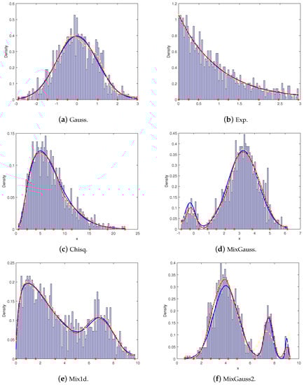
Figure 2.
Density estimates use uniform and nonuniform B-splines. The blue rectangle represents the histogram, the blue solid line represents the true density function, the yellow dashed line represents the uniform B-spline function, and the red dotted line represents the adaptive nonuniform B-spline function. The knots of the nonuniform B-splines are marked as asterisks along the horizontal axis.
When the sample size was fixed, the errors of the uniform B-spline and the nonuniform B-spline are compared in Table 2. The measured entropy (ME), the information entropy (H), the mean absolute error (MAE), the mean square error (root-MSE), and the Bayesian information criterion (BIC) scores are listed, which demonstrated that the adaptive nonuniform B-spline estimators usually outperformed the uniform B-spline estimators. In addition, compared to the uniform B-spline estimators, the adaptive nonuniform B-spline estimators were usually closer to the true density functions, which is shown in Figure 2.
When the sample size varied as , 100, 500, 1000, 5000, the root-MSE and MAE results are listed for the uniform B-spline estimators and the nonuniform estimators in Table 3. From the ratio of the MAE and root-MSE, we can see that the fitting results of the adaptive nonuniform B-spline outperformed those of the uniform B-spline.
Table 3.
Uniform vs. non-uniform . The goodness of fit for data using the uniform B-spline and nonuniform B-spline with the different sample sizes.
5.3. Comparison with Orthogonal Sequence and Kernel Estimators
Table 4 and Table 5 show the results compared with the previously mentioned probability density function estimation methods, including the orthogonal sequence of [7,13], the kernel estimators using three strategies to the bandwidth selected, that is, the rule-of-thumb method, which is based on the asymptotic mean integrated square error (ROT) [38], the least squares cross-validation method (LCV) [38], and a method proposed by Hall et al. based on the straightforward idea of plugging estimates into the usual asymptotic representation for the optimal bandwidth but with two important modifications (HALL) [39]. The experimental results of the B-spline function estimation used the values of the MAE and root-MSE.
Table 4.
The goodness of fit for data using the nonuniform B-spline methods, orthogonal sequence, and kernel estimators (The number of sample points is 1000).
Table 5.
The goodness of fit using the nonuniform B-spline, orthogonal sequence, and kernal estimators with the different sample sizes.
In Table 4, we observe that with the same sample size, the errors of the nonuniform B-spline were smaller. The errors of the root-MSE and MAE of the nonuniform B-spline were smaller than those of the other methods, which showed that the estimation effect of the adaptive nonuniform B-splines was better than that of the listed methods. In addition, the fitting results obtained by the nonuniform B-splines overcame the overfitting phenomenon of the uniform method.
In Table 5, the error analysis of different sample sizes for the nonuniform B-spline, orthogonal sequence, and kernel methods are listed. The experimental results showed that the errors of the nonuniform B-spline were smaller, and the errors became smaller with the increase in the sample size. It was also shown that the B-spline fitting method of the nonuniform knots generated by our adaptive strategy had a better fitting effect.
6. Conclusions
In this work, we introduced a novel density estimation with nonuniform B-splines. By introducing the error indicator attached to each interval for density estimation, we proposed an adaptive strategy to generate the nonuniform knot vector. The numerical experiments showed that, compared with the uniform B-spline, the local density estimation with nonuniform B-splines not only achieved better estimation results but also effectively alleviated the overfitting phenomenon caused by the uniform B-splines. The comparison with the existing estimation procedures, including the state-of-the-art kernel estimators, demonstrated the accuracy of our new method.
In the future, it would be interesting to extend the method considered in the paper to multivariate density cases. Another natural direction to pursue further is the fast automatic knot placement method via feature characterization from the samples, which can generate the nonuniform knot vector directly. We leave these topics for future research.
Author Contributions
Y.Z., M.Z., Q.N. and X.W. had equal contributions. All authors have read and agreed to the published version of the manuscript.
Funding
This work was supported by the National Natural Science Foundation of China No.122011292 and No.61772167.
Institutional Review Board Statement
Not applicable.
Informed Consent Statement
Not applicable.
Data Availability Statement
Not applicable.
Conflicts of Interest
The authors declare no conflict of interest.
References
- Siegel, S. Nonparametric statistics. Am. Stat. 1957, 11, 13–19. [Google Scholar]
- Gibbons, J.D.; Chakraborti, S. Nonparametric Statistical Inference; CRC Press: Boca Raton, FL, USA, 2014. [Google Scholar]
- García, S.; Luengo, J.; Sáez, J.A.; López, V.; Herrera, F. A survey of discretization techniques: Taxonomy and empirical analysis in supervised learning. IEEE Trans. Knowl. Data Eng. 2013, 25, 734–750. [Google Scholar] [CrossRef]
- Bhattacharya, A.; Dunson, D.B. Nonparametric Bayesian density estimation on manifolds with applications to planar shapes. Biometrika 2010, 97, 851–865. [Google Scholar] [CrossRef] [PubMed]
- Hall, P. Cross-validation and the smoothing of orthogonal series density estimators. J. Multivar. Anal. 1987, 21, 189–206. [Google Scholar] [CrossRef]
- Dai, X.; Müller, H.-G.; Yao, F. Optimal bayes classifiers for functional data and density ratios. Biometrika 2017, 104, 545–560. [Google Scholar]
- Leitao, Á.; Oosterlee, C.W.; Ortiz-Gracia, L.; Bohte, S.M. On the data-driven cos method. Appl. Math. Comput. 2018, 317, 68–84. [Google Scholar] [CrossRef]
- Ait-Hennani, L.; Kaid, Z.; Laksaci, A.; Rachdi, M. Nonparametric estimation of the expected shortfall regression for quasi-associated functional data. Mathematics 2022, 10, 4508. [Google Scholar] [CrossRef]
- Terrell, G.R.; Scott, D.W. Variable kernel density estimation. Ann. Stat. 1992, 1236–1265. [Google Scholar] [CrossRef]
- Lamnii, A.; Nour, M.Y.; Zidna, A. A reverse non-stationary generalized b-splines subdivision scheme. Mathematics 2021, 9, 2628. [Google Scholar] [CrossRef]
- Fan, J.; Gijbels, I. Local Polynomial Modelling and Its Applications; Routledge: London, UK, 2018. [Google Scholar]
- Redner, R.A. Convergence rates for uniform B-spline density estimators part i: One dimension. SIAM J. Sci. Comput. 1999, 20, 1929–1953. [Google Scholar] [CrossRef]
- Cui, Z.; Kirkby, J.L.; Nguyen, D. Nonparametric density estimation by b-spline duality. Econom. Theory 2020, 36, 250–291. [Google Scholar] [CrossRef]
- Cui, Z.; Kirkby, J.L.; Nguyen, D. A data-driven framework for consistent financial valuation and risk measurement. Eur. J. Oper. Res. 2021, 289, 381–398. [Google Scholar] [CrossRef]
- Cui, Z.; Kirkby, J.L.; Nguyen, D. Efficient simulation of generalized sabr and stochastic local volatility models based on markov chain approximations. Eur. J. Oper. Res. 2021, 290, 1046–1062. [Google Scholar] [CrossRef]
- Kooperberg, C.; Stone, C.J. Comparison of parametric and bootstrap approaches to obtaining confidence intervals for logspline density estimation. J. Comput. Graph. Stat. 2004, 13, 106–122. [Google Scholar] [CrossRef]
- Koo, J.-Y. Bivariate b-splines for tensor logspline density estimation. Comput. Stat. Data Anal. 1996, 21, 31–42. [Google Scholar] [CrossRef]
- Gu, C. Smoothing spline density estimation: A dimensionless automatic algorithm. J. Am. Stat. Assoc. 1993, 88, 495–504. [Google Scholar] [CrossRef]
- Eilers, P.H.; Marx, B.D. Flexible smoothing with b-splines and penalties. Stat. Sci. 1996, 11, 89–121. [Google Scholar] [CrossRef]
- Papp, D.; Alizadeh, F. Shape-constrained estimation using nonnegative splines. J. Comput. Graph. Stat. 2014, 23, 211–231. [Google Scholar] [CrossRef]
- Kirkby, J.L.; Leitao, Á.; Nguyen, D. Nonparametric density estimation and bandwidth selection with b-spline bases: A novel galerkin method. Comput. Stat. Data Anal. 2021, 159, 107202. [Google Scholar] [CrossRef]
- Oliveira, M.; Crujeiras, R.M.; Rodríguez-Casal, A. A plug-in rule for bandwidth selection in circular density estimation. Comput. Stat. Data Anal. 2012, 56, 3898–3908. [Google Scholar] [CrossRef]
- Boente, G.; Rodriguez, D. Robust bandwidth selection in semiparametric partly linear regression models: Monte carlo study and influential analysis. Comput. Stat. Data Anal. 2008, 52, 2808–2828. [Google Scholar] [CrossRef]
- Hall, P.; Kang, K.-H. Bandwidth choice for nonparametric classification. Ann. Stat. 2005, 33, 284–306. [Google Scholar] [CrossRef]
- Loader, C. Bandwidth selection: Classical or plug-in? Ann. Stat. 1999, 27, 415–438. [Google Scholar] [CrossRef]
- Boor, C.D.; Boor, C.D. A Practical Guide to Splines; Springer: New York, NY, USA, 1978; Volume 27. [Google Scholar]
- Farin, G. Curves and Surfaces for Computer-Aided Geometric Design: A Practical Guide; Elsevier: Amsterdam, The Netherlands, 2014. [Google Scholar]
- Ezhov, N.; Neitzel, F.; Petrovic, S. Spline approximation, part 2: From polynomials in the monomial basis to b-splines—A derivation. Mathematics 2021, 9, 2198. [Google Scholar] [CrossRef]
- Curry, H.B.; Schoenberg, I.J. On spline distributions and their limits-the polya distribution functions. Bull. Am. Math. Soc. 1947, 53, 1114. [Google Scholar]
- Lyche, T.; Manni, C.; Speleers, H. Foundations of spline theory: B-splines, spline approximation, and hierarchical refinement. In Splines and PDEs: From Approximation Theory to Numerical Linear Algebra; Springer: Berlin/Heidelberg, Germany, 2018; pp. 1–76. [Google Scholar]
- Zong, Z.; Lam, K. Estimation of complicated distributions using B-spline functions. Struct. Saf. 1998, 20, 341–355. [Google Scholar] [CrossRef]
- López-Cruz, P.L.; Bielza, C.; Larranaga, P. Learning mixtures of polynomials of multidimensional probability densities from data using b-spline interpolation. Int. J. Approx. Reason. 2014, 55, 989–1010. [Google Scholar] [CrossRef]
- Loock, W.V.; Pipeleers, G.; Schutter, J.D.; Swevers, J. A convex optimization approach to curve fitting with b-splines. IFAC Proc. Vol. 2011, 44, 2290–2295. [Google Scholar] [CrossRef]
- Bastian, P.; Wittum, G. Adaptive multigrid methods: The ug concept. In Adaptive Methods—Algorithms, Theory and Applications; Springer: Berlin/Heidelberg, Germany, 1994; pp. 17–37. [Google Scholar]
- Urth, R.V. A Review of a Posteriori Error Estimation and Adaptive Mesh-Refinement Techniques; BG Teubner: Leipzig, Germany, 1996. [Google Scholar]
- Dörfel, M.R.; Jüttler, B.; Simeon, B. Adaptive isogeometric analysis by local h-refinement with t-splines. Comput. Methods Appl. Mech. Eng. 2010, 199, 264–275. [Google Scholar] [CrossRef]
- Morin, P.; Nochetto, R.H.; Siebert, K.G. Data oscillation and convergence of adaptive fem. SIAM J. Numer. Anal. 2000, 38, 466–488. [Google Scholar] [CrossRef]
- Węglarczyk, S. Kernel density estimation and its application. In ITM Web of Conferences; EDP Sciences: Les Ulis, France, 2018; p. 00037. [Google Scholar]
- Troudi, M.; Alimi, A.M.; Saoudi, S. Analytical plug-in method for kernel density estimator applied to genetic neutrality study. EURASIP J. Adv. Signal Process. 2008, 2008, 1–8. [Google Scholar] [CrossRef]


Disclaimer/Publisher’s Note: The statements, opinions and data contained in all publications are solely those of the individual author(s) and contributor(s) and not of MDPI and/or the editor(s). MDPI and/or the editor(s) disclaim responsibility for any injury to people or property resulting from any ideas, methods, instructions or products referred to in the content. |
© 2023 by the authors. Licensee MDPI, Basel, Switzerland. This article is an open access article distributed under the terms and conditions of the Creative Commons Attribution (CC BY) license (https://creativecommons.org/licenses/by/4.0/).